Rule Extraction
Johan Huysmans1, Bart Baesens1,2 and Jan Vanthienen1
1
K.U.Leuven, Dept. of Decision Sciences and Information Management, Naamsestraat 69, B-3000 Leuven, Belgium
2
School of Management, University of Southampton, Southampton, SO17 1BJ, United Kingdom
Abstract. Various benchmarking studies have shown that artificial neu-ral networks and support vector machines have a superior performance when compared to more traditional machine learning techniques. The main resistance against these newer techniques is based on their lack of interpretability: it is difficult for the human analyst to understand the motivation behind these models’ decisions. Various rule extraction tech-niques have been proposed to overcome this opacity restriction. However, most of these extraction techniques are devised for classification and only few algorithms can deal with regression problems.
In this paper, we present ITER, a new algorithm for pedagogical re-gression rule extraction. Based on a trained ‘black box’ model, ITER is able to extract human-understandable regression rules. Experiments show that the extracted model performs well in comparison with CART regression trees and various other techniques.
1
Introduction
While newer machine learning techniques, like artificial neural networks and sup-port vector machines, have shown superior performance in various benchmarking studies [1,10] the application of these techniques remains largely restricted to re-search environments. A more widespread adoption of these techniques is foiled by their lack of explanation capability which is required in some application ar-eas, like medical diagnosis or credit scoring. To overcome this restriction, various algorithms [2,4,5,6,8] have been proposed to extract meaningful rules from such trained ‘black box’ models. These algorithms’ dual goal is to mimic the behavior of the black box as closely as possible with a minimal amount of rules. The main part of these extraction algorithms focus on classification problems, with only a few exceptions devised especially for regression.
In this paper, we present ITER, a new algorithm for pedagogical regression rule extraction. Based on a trained ‘black box’ model ITER is able to extract human-understandable regression rules. The algorithm works by iteratively ex-panding a number of hypercubes until the entire input space is covered.
In the next section, a small overview of related research is given. While al-gorithms for classification rule extraction are more widespread, we will cover
A Min Tjoa and J. Trujillo (Eds.): DaWaK 2006, LNCS 4081, pp. 270–279, 2006. c
some techniques that are able to extract regression rules either directly from the data points or from an underlying ‘black box’ regressor. In the third sec-tion, the inner workings of the ITER algorithm are explained in great detail and the performance of this algorithm is compared with other machine learning techniques.
2
Related Research
Regression trees [3,7] are usually constructed directly from the available training observations and are therefore not considered to be rule extraction techniques in the strict sense of the word. A CART regression tree [3] is a binary tree with conditions specified next to each non-leaf node. Classifying a new observation is done by following the path from the root towards a leaf node, choosing the left node when the condition is satisfied and the right node otherwise, and assigning the observation the value below the leaf node. This value below the leaf nodes equals the average y-value of training observations falling into this leaf node.
The regression tree is constructed by iteratively splitting nodes, starting from only the root node, so as to minimize an impurity measure. Often, the impurity measure of a node t is calculated as:
R(t) = 1
N
xn∈t
(yn−y(t))2 (1)
with (xn, yn) the training observations andy(t) the average y-value for observa-tions falling into node t. The best split for a leaf-node of the tree is chosen such that it minimizes the impurity of the newly created nodes. Mathematically, the best split s* of a node t is that split s which maximizes:
ΔR(s, t) =R(t)−pLR(tL)−pRR(tR) (2) withtL andtRthe newly created nodes. Construction of the tree is terminated when certain stopping criteria are met. Pruning of the nodes is performed after-wards to improve generalization behavior of the constructed tree.
Although most regression tree algorithms can be applied directly on the train-ing data, it is also possible to apply these techniques for pedagogical rule extrac-tion. Instead of using the original targets, the target values are provided by a trained black box model and the regression tree is constructed on these new data points. In our empirical experiments, we will use CART with both approaches.
3
ITER
3.1 Description
The pedagogical ITER-algorithm1 can be used to build predictive regression rules from a trained regression model (e.g., a neural network or support vector
machine). With minor adaptations it is suitable for classification problems as well. The main idea of the algorithm is to iteratively expand a number of (hy-per)cubes until they cover the entire input space. Each of these cubes can then be converted into a rule of the following format:
if Var 1∈[ValueLow1 ,ValueHigh1 ] and Var 2∈[ValueLow2 ,ValueHigh2 ]
. . .and Var M∈[ValueLowM ,ValueHighM ] then predict some Constant with M the dimension of the input space. The algorithm starts with the creation of a user-defined number of random starting cubes. These cubes are infinitesi-mally small and therefore correspond to points in the input space. Afterwards, these initial cubes are gradually expanded until they cover the entire input space or until they can no longer be expanded. During each update the following steps are executed:
1. For each hypercube i=1,. . . ,N and for each dimension j=1,. . . ,M calculate how far the cube can be expanded to both extremes of the dimension be-fore it intersects with another cube, call these distances LowerLimitji and
U pperLimitji.
2. For each hypercube i=1,. . . ,N and for each dimension j=1,. . . ,M calculate the size of the update. The update equalsM inU pdatej, a user-specified con-stant, unless this size would result in overlapping cubes. If this is the case then the update is smaller such that the two blocks become adjacent. Mathematically: LowerU pdateji= minimum{LowerLimitji, M inU pdatej} andU pperU pdateji = minimum{U pperLimitji,M inU pdatej}
3. For each hypercube i=1,. . . ,N and for each dimension j=1,. . . ,M create two temporary cubes adjacent to the original cube along the opposite sides of dimension j with a width of respectivelyLowerU pdateji andU pperU pdateji. For each of both cubes, create a number of random points lying within the cube and calculate the mean prediction for these points according to the trained continuous regression model. Call the difference between each of both means and the mean prediction for the original cube respectively
LowerDif fij andU pperDif fij.
4. Find the global minimum over all cubes of these differences and combine the temporary cube for which the difference was minimal with its original cube. Update the mean prediction for this cube and remove all other temporary cubes.
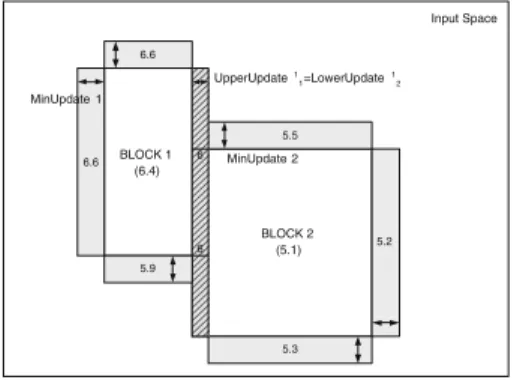
A small example will help to clarify the above procedure. In Figure 1, a two-dimensional input space (M=2) is shown with two cubes (N=2). We have chosen
M inU pdate1 equal to M inU pdate2, a small positive constant. The numbers within the cubes are the mean predictions of the continuous black box model for points lying within that cube.
For both cubes we create four new cubes that surround the original cube. In Figure 1, these cubes are dark-shaded. The height of the cubes on the top and bottom (expanding along Y-dimension) equalsM inU pdate2. Similarly, the
BLOCK 2 (5.1) 5.2 5.3 5 5.5 Input Space BLOCK 1 (6.4) 6 6 5.9 6.6 6.6 MinUpdate 2 MinUpdate 1 UpperUpdate1 1=LowerUpdate12
Fig. 1.Example for Iter-algorithm
width of the cubes on the left and right equals M inU pdate1. However, if the first cube is expanded M inU pdate1 units to the right, it would overlap with the second cube. Therefore the update to the right is smaller so that the two blocks become adjacent and non-overlapping. The same situation occurs with the update of the second block to the left (striped regions in Figure 1). For each of the dark shaded cubes, a number of random observations lying within that cube are generated and the predictions of the original ‘black box’ model for these data points are averaged. Finally, we select the shaded cube for which the difference between this average and the average prediction for the original cube is minimal. In the example, this is the shaded cube most to the right with a difference of 0.1. This cube is then combined with its original cube and the mean prediction for this cube is updated. The above steps are iterated until no further updates are possible.
3.2 Discussion
Size of Input Space. Before the first iteration of the algorithm, ITER
calcu-lates the size of the surrounding hypercube, i.e. the cube that surrounds all of the training observations. When calculating the allowed update size, ITER takes this surrounding cube into consideration and never creates cubes that lie out-side the surrounding cube. The surrounding cube is also used to retrieve default values for the M inU pdatej’s. Unless the user specifies otherwise, the defaults equal a twentieth of the size of each dimension. For example, if the values of the training observations for some dimension lie within the interval [0,1] then
M inU pdate=0.05.
Non-exhaustivity
While ITER creates rules that are non-overlapping, it is not always able to cover the entire input space. With other words, the rules created by ITER are exclusive but not necessarily exhaustive. In Figure 4(f), a small example of this situation is given. None of the four cubes can expand towards the middle because each cube is blocked by another cube. The shaded area will therefore not be covered by any rule. To ensure exhaustivity, we have to add a number of cubes that cover
the remaining gaps. Fortunately, from initial experiments we have observed that generally the number of cubes to add remains relatively small.
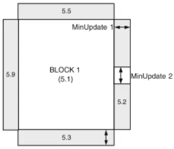
New Cube Creation
By specifying the number of starting cubes, the user automatically indicates the desired number of rules because ITER will never create extra cubes during exe-cution. Only to make the resulting rule set exhaustive, the algorithm is allowed to construct additional cubes. There are several disadvantages, such as a strong dependence of the results on the number and location of the starting cubes, that make it worthwhile to give the algorithm the opportunity to create a new cube when the current update is deemed not ‘good’ enough. In this definition, we con-sider an update to be ‘good’ when the global minimum of step 4 is smaller than a user-specified threshold. We will therefore modify step 4 of the algorithm to:
New Step 4
Find the global minimum over all cubes of these differences.
– If this global minimum is smaller than the threshold then combine the tempo-rary cube for which the difference was minimal with its original cube. Update the mean prediction for this cube and remove all other temporary cubes.
– If this global minimum is larger than the threshold then create a new cube on the position of the temporary cube for which the difference was the global minimum. The size of each side of the hypercube equalsM inimumU pdatej (smaller if this results in overlapping cubes)
BLOCK 1 (5.1) 5.2 5.3 5.5 MinUpdate 1 MinUpdate 2 5.9
Fig. 2.New Cube Creation
By setting the threshold to a very large value, all updates will be considered good and the results of the updated step 4 will be similar to the original. In Figure 2, the creation of a new cube is shown. When the threshold is smaller than 0.1, a new cube will be created at the right hand side of the original cube. The size of each dimension of this new cube equalsM inU pdatej.
4
Empirical Results
In this section, ITER is applied to several artificial datasets with 2 continuous inputs from the interval [0,1]. Each of the datasets consists of 1000 observations, 500 for training and 500 for testing, and implements the following rules:
Table 1.Datasets
ARTI1 ARTI2
if x≤0.5 and y≤0.5 then z=0.7 +αRAND if x≤0.5 and y≤0.5 then z=0 +αRAND if x≤0.5 and y>0.5 then z=0.4 +αRAND if x≤0.5 and y>0.5 then z=1 +αRAND if x>0.5 and y≤0.5 then z=0.3 +αRAND if x>0.5 and y≤0.5 then z=1 +αRAND if x>0.5 and y>0.5 then z=0.0 +αRAND if x>0.5 and y>0.5 then z=0 +αRAND
ARTI3 ARTI4
z= x + y +αRAND z= 1−(x−0.5)2−(y−0.5)2+αRAND
a linear function a parabole
with RAND a uniform random number in the interval [-1,1] andαa parameter to control the amount of randomness in the data. Although ARTI1 and ARTI2 may seem very similar, the symmetry in ARTI2 will cause considerable problems for a greedy algorithm like CART.
Several models are evaluated for each of these datasets and the influence of noise is tested by applying different values forα. The different models are Lin-ear Regression (LR), K-NLin-earest Neighbor (KNN), Least-Squares Support Vec-tor Machines (LS-SVM) [9] and CART. For the LS-SVMs we use a RBF-kernel with regularization and kernel parameters selected by a gridsearch procedure as described in [9]. CART trees were applied both directly on the data and as a pedagogical algorithm. For the pedagogical approach, we replace the original tar-gets with values provided by the best performing ‘black box’, usually a LS-SVM model. Subsequent pruning of the tree is performed by minimizing the 10-fold cross-validation error on the training data to improve generalization behavior of the tree.
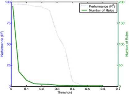
For a comparison of ITER with the other models, we initialize the algorithm with one random start cube and the default update sizes. For the selection of an appropriate threshold value, a simple trial-and-error approach was followed. For different values of the threshold we plot the average number of extracted rules and the performance on the training data over 100 independent trials. In Figure 3, we show this plot for ARTI 1 withαset to 0. It can be observed that small values for the threshold result in better performance but that it comes at the cost of an increased number of rules. A threshold somewhere between 0.1 and 0.25 might be preferred as it provides both interpretability and accuracy. Notice
0 0.1 0.2 0.3 0.4 0.5 0.6 0.7 0 25 50 75 100 Performance (R 2) Threshold 0 0.1 0.2 0.3 0.4 0.5 0.6 0.70 50 100 150 200 Number of Rules Performance (R2) Number of Rules
0 0.5 1 0 0.5 1 −0.2 0 0.2 0.4 0.6 0.8 (a) LS-SVM Model 0 0.5 1 0 0.5 1 −0.2 0 0.2 0.4 0.6 0.8
(b) Extracted Rules (threshold=0.2)
0 0.1 0.2 0.3 0.4 0.5 0.6 0.7 0.8 0.9 1 0 0.1 0.2 0.3 0.4 0.5 0.6 0.7 0.8 0.9 1 1
(c) Initial Cube (After 2 Updates)
0 0.1 0.2 0.3 0.4 0.5 0.6 0.7 0.8 0.9 1 0 0.1 0.2 0.3 0.4 0.5 0.6 0.7 0.8 0.9 1 1 2 (d) After 25 Updates 0 0.1 0.2 0.3 0.4 0.5 0.6 0.7 0.8 0.9 1 0 0.1 0.2 0.3 0.4 0.5 0.6 0.7 0.8 0.9 1 1 2 3
(e) After 50 Updates
0 0.1 0.2 0.3 0.4 0.5 0.6 0.7 0.8 0.9 1 0 0.1 0.2 0.3 0.4 0.5 0.6 0.7 0.8 0.9 1 1 2 3 4 (f) After 84 Updates
Fig. 4.Original LS-SVM Model (a) and extracted rules (b) for ARTI1 (α= 0)
that the choice for a small threshold will result in rules that better approximate the underlying ‘black box’ model but that it will not lead to overfitting as long as the underlying model generalizes well. In Figure 4, execution of the algorithm is shown for ARTI1 with the threshold set to 0.2.
In Table 2, an overview of the results is given. For each of the models, we calculate the Mean Absolute Error (MAE) andR2 value as follows:
M AE= 1 N N i=1 |yi−yˆi| (3)
R2= 1− N i=1(yi−yˆi)2 N i=1(yi−y¯)2 (4) with N the number of observations,yi and ˆyi respectively the target value and model prediction for observation i and ¯y the mean target value. For the rule extraction techniques, MAE Fidelity andR2 Fidelity show to what extent the
extracted rules mimic the behavior of the underlying model. The same formu-las (3) and (4) were used to calculate these measures, but with yi and ˆyi rep-resenting the model prediction of respectively the ‘black box’ model and the extracted rules.
From Table 2, one can conclude that ITER is able to mimic accurately the behavior of the underlying models with only a limited amount of rules. For several of the experiments, ITER even achieves the same level of performance
Table 2.Overview of Out-of-Sample Performance
MAE R2 # Rules MAE Fidel.R2Fidel. MAE R2 # Rules MAE Fidel.R2Fidel.
ARTI1(α=0) ARTI1(α=0.5) LR 0.11 74.79 0.27 32.61 KNN(k=5) 0.02 93.10 0.27 27.90 LS-SVM 0.03 94.93 0.27 35.28 CARTdirect 0.00 99.52 4 0.26 37.99 4 CARTLS−SV M 0.01 97.41 12.95 0.02 97.80 0.26 36.26 51.31 0.03 97.47 IT ERthreshold=0.05 LS−SV M 0.02 94.93 36.25 0.02 98.61 0.26 35.73 73.33 0.03 97.45 IT ERthreshold=0.1 LS−SV M 0.02 95.12 12.94 0.02 97.75 0.26 35.74 16.40 0.05 91.19 IT ERthreshold=0.2 LS−SV M 0.03 90.73 4.50 0.04 93.54 0.27 32.30 4.98 0.08 79.90 ARTI2(α=0) ARTI2(α=0.5) LR 0.50 -0.65 0.48 -0.45 KNN(k=5) 0.05 92.18 0.30 59.15 LS-SVM 0.01 95.20 0.29 61.75 CARTdirect 0.00 98.40 11.96 0.27 68.15 11.01 CARTLS−SV M 0.01 97.11 11.35 0.01 96.15 0.28 65.38 41.20 0.07 96.27 IT ERthreshold=0.1 LS−SV M 0.04 92.85 31.55 0.03 93.51 0.29 62.13 82.59 0.07 96.36 IT ERthreshold=0.15 LS−SV M 0.04 92.94 26.72 0.03 93.43 0.29 63.48 35.64 0.08 94.31 IT ERthreshold=0.20 LS−SV M 0.04 92.79 21.20 0.04 93.31 0.29 63.03 18.88 0.10 91.56 ARTI3(α=0) ARTI3(α=0.5) LR 0.02 99.50 0.26 63.81 KNN(k=5) 0.03 99.17 0.28 56.74 LS-SVM 0.03 99.49 0.26 63.75 CARTdirect 0.05 97.48 86.41 0.28 55.65 15.11 CARTLS−SV M 0.06 97.09 74.88 0.05 97.75 0.26 63.68 77.10 0.04 98.19 IT ERthreshold=0.05 LS−SV M 0.04 98.63 190.25 0.03 99.16 0.26 63.18 162.31 0.03 99.08 IT ERthreshold=0.10 LS−SV M 0.07 96.08 51.90 0.06 96.61 0.27 61.54 44.58 0.06 96.35 IT ERthreshold=0.15 LS−SV M 0.09 92.24 25.00 0.09 92.76 0.27 58.51 22.33 0.09 92.27 IT ERthreshold=0.2 LS−SV M 0.12 87.02 15.34 0.12 87.53 0.28 54.98 13.39 0.11 87.11 ARTI4(α=0) ARTI4(α=0.25) LR 0.08 -0.39 0.14 0.52 KNN(k=5) 0.01 98.22 0.14 17.76 LS-SVM 0.00 100.00 0.13 26.70 CARTdirect 0.02 94.27 92.08 0.14 17.56 14.48 CARTLS−SV M 0.02 93.49 59.15 0.02 93.50 0.13 24.35 65.09 0.02 94.59 IT ERthreshold=0.04 LS−SV M 0.02 92.58 68.60 0.02 92.59 0.13 24.57 75.02 0.02 93.68 IT ERthreshold=0.05 LS−SV M 0.03 88.71 44.82 0.03 88.71 0.13 23.22 49.00 0.03 90.24 IT ERthreshold=0.1 LS−SV M 0.05 63.32 10.99 0.05 63.33 0.14 17.72 11.97 0.05 67.32
as the underlying black box models. However, one can also observe that ITER has difficulties with finding the exact boundaries when the update size is chosen too large. For example, in Figure 4(f) ITER makes the first cube too large along the Y-axis because it uses the default update size of 0.05. A smaller update size would allow for better performance but at the cost of an increase in iterations and computation time. We are therefore looking into the use of adaptive update sizes so that larger updates are applied when the underlying ‘black box’ function is flat and smaller update sizes when the algorithm encounters slopes.
The results show that CART slightly outperforms ITER on most datasets, but what can not be observed from the results is the advantage of ITER’s non-greedy approach for the interpretability of the extracted rules. For example, CART will fail to find good rules for ARTI2 because it is unable to find a split for the root node that significantly decreases impurity. It will therefore choose a more-or-less random split, x2<0.95, that does not correspond to any of the optimal splits (x1<0.5 or x2<0.5). ITER’s expanding of hypercubes does not face this problem of looking only one step ahead and will be able to find rules that correspond more closely to those of Table 1.
5
Conclusion
In this paper, we presented a new algorithm for regression rule extraction and compared its performance with CART regression trees and several ‘black box’ regression techniques. While we believe that ITER can become a worthwhile alternative to CART’s recursive partitioning approach, there is one major im-provement recommended before ITER is able to assume this role. The use of adaptive update sizes can increase performance of the extracted rules in combi-nation with a reduction of the required number of iterations. Our current work is focused on the implementation of this adaptive update rates. Future research will expand the algorithm to allow nominal variables as inputs and consequents for the rules that can be linear functions of the inputs.
References
1. B. Baesens, T. Van Gestel, S. Viaene, M. Stepanova, J. Suykens, and J. Vanthienen. Benchmarking state of the art classification algorithms for credit scoring. Journal of the Operational Research Society, 54(6):627–635, 2003.
2. N. Barakat and J. Diederich. Eclectic rule-extraction from support vector machines. International Journal of Computational Intelligence, 2(1):59–62, 2005.
3. L. Breiman, J.H. Friedman, R.A. Olsen, and C.J. Stone.Classification and Regres-sion Trees. Wadsworth and Brooks, 1984.
4. G. Fung, S. Sandilya, and R.B. Rao. Rule extraction from linear support vector machines. In11th ACM SIGKDD international conference on Knowledge discovery in data mining, pages 32–40, 2005.
5. D. Martens, B. Baesens, T. Van Gestel, and J. Vanthienen. Adding comprehensibil-ity to support vector machines using rule extraction techniques. InCredit Scoring and Credit Control IX, 2005.
6. H. N´u˜nez, C. Angulo, and A. Catal`a. Rule extraction from support vector machines. InEuropean Symposium on Artificial Neural Networks (ESANN), pages 107–112, 2002.
7. J.R. Quinlan. Learning with Continuous Classes. In5th Australian Joint Confer-ence on Artificial IntelligConfer-ence, pages 343–348, 1992.
8. R. Setiono, W.K. Leow, and J.M. Zurada. Extraction of rules from artificial neu-ral networks for nonlinear regression. IEEE Transactions on Neural Networks, 13(3):564–577, 2002.
9. J.A.K. Suykens, T. Van Gestel, J. De Brabanter, B. De Moor, and J. Vandewalle. Least Squares Support Vector Machines. World Scientific, Singapore, 2002. 10. S. Viaene, R. Derrig, B. Baesens, and G. Dedene. A comparison of state-of-the-art
classification techniques for expert automobile insurance fraud detection. Journal of Risk And Insurance (Special Issue on Fraud Detection), 69(3):433–443, 2002.