DOCUMENT DE TREBALL
XREAP2011-12
A correlation sensitivity analysis of non-life
underwriting risk in solvency capital requirement
estimation
Lluís Bermúdez (RFA-IREA)
Antoni Ferri (RFA-IREA)
Montserrat Guillén (RFA-IREA)
A
correlation
sensitivity
analysis
of
non
‐
life
underwriting
risk
in
solvency
capital
requirement
estimation
Lluís Bermúdeza
, Antoni Ferrib1
and Montserrat Guillénb a
Departament de Matemàtica Econòmica, Financera i Actuarial. RISC‐IREA. University of Barcelona. Spain b
Departament d'Econometria, Estadística i Economia Espanyola. RISC‐IREA. University of Barcelona. Spain
Abstract:
This paper analyses the impact of using different correlation assumptions between lines of business when estimating the risk‐based capital reserve, the Solvency Capital
Requirement (SCR), under Solvency II regulations. A case study is presented and the SCR is calculated according to the Standard Model approach. Alternatively, the requirement is then calculated using an Internal Model based on a Monte Carlo simulation of the net underwriting result at a one‐year horizon, with copulas being used to model the dependence between lines of business. To address the impact of these model assumptions on the SCR we conduct a sensitivity analysis. We examine changes in the correlation matrix between lines of business and address the choice of copulas. Drawing on aggregate historical data from the Spanish non‐life insurance market between 2000 and 2009, we conclude that modifications of the correlation and dependence assumptions have a significant impact on SCR estimation.
Keywords: Solvency II, Solvency Capital Requirement, Standard Model, Internal Model, Monte Carlo simulation, Copulas.
1
Motivation
and
Aims
The European insurance regulator seeks to obtain a global vision of each insurance company operating in the EU. For that purpose, quantitative tools are used to estimate the economic value of the aggregate risk assumed by a company. The European Directive 2009/138/EC, generally known as Solvency II, provides a common legal frame for companies based in any of the EU member states to operate in the insurance and reinsurance business. Solvency II establishes capital requirements to ensure stability against unexpected adverse fluctuations, and so it guarantees policyholder protection by means of two capital reserves: Minimum Solvency Capital Requirement (MSCR) and
Solvency Capital Requirement (SCR). These capital reserve funds have to be calculated by each company or insurance group according to the so‐called Standard Model, or with the regulator's previous authorization, according to an Internal Model.
1
Corresponding Author. Departament d'Econometria, Estadística i Economia Espanyola, Universitat de
Barcelona, Diagonal 690, 08034‐Barcelona, Spain. Tel.:+34‐93‐4037043 fax: +34‐93‐4021821; e‐mail:
Under Solvency II, the SCR is estimated following a modular structure of risks related to insurance activity, including underwriting, market, credit and operational risks. In this paper, we focus on non‐life underwriting risk, for which the Directive imposes a capital requirement that must consider at least a level of granularity by lines of business.
Thus, the presence of several lines of business within a company is taken into account when calculating the SCR. Furthermore, these lines of business are not necessarily assumed to be statistically independent. A hypothesis can thus be established regarding the association between the results of different lines of business within the same company. Indeed, significant correlations may be present as a result of both endogenous and exogenous causes. For instance, when a company has several lines of business that cover risks in a specific geographic region or when it operates in the same economic environment, positive correlations between the net underwriting results of certain lines of business are possible. Correlation between lines of business is a hot topic in insurance and we think that the consequences of ignoring that correlation have not been fully addressed. Gisler and Bühlmann (2005) present the theory of multivariate credibility in their book. Some authors, like Englund el al. (2008), have tried to develop pricing rules that take into account the interrelations between several lines of business for those cases where a policyholder has, or may have, several insurance contracts within an insurance company.
Our aim is to compare the SCR results for the non‐life underwriting risk module obtained using the Standard and Internal Models, with particular attention to the influence of the hypothesis made regarding the correlation matrix between lines of business2. More generally, we examine the dependence structure. Using the standard formula and the parameters suggested by the 5th Quantitative Impact Study (QIS‐5) and assuming a simple internal model with an alternative dependence hypothesis, we carry out a sensitivity analysis on the correlation matrix assumptions when calculating the capital requirement for non‐life underwriting risk.
For the non‐life underwriting risk module, the SCR based on the Solvency II
Standard Model is established mainly by the parameters provided by the Committee of European Insurance Supervisors (CEIOPS)3. These parameters include standard deviations for a mix of premium and reserve risks and a correlation matrix between lines of business. However, an Internal Model for solvency does not necessarily have to be based on a modular structure, although we retain modules in our model so that we might estimate a capital comparable to that obtained for the non‐life underwriting risk module under the standard approach. For comparative purposes, we propose a basic internal model based on linear regression techniques and copulas. Then, assuming a set of hypotheses on the correlations between lines of business we estimate economic capital requirements under a variety of scenarios.
Using aggregate historical data from the Spanish non‐life insurance market, we find that the SCR based on the Solvency II Standard Model overestimates the capital
2
Our work is related to the work by Filipović (2009), but he concentrates on risk types rather than lines of
business.
3
obtained from the Internal Model in almost all cases considered. We also conclude that modifications of the correlation and dependence assumptions have a significant impact on SCR estimation. Several studies related to SCR estimation can be found in the literature. Sandström (2007) reports the effect of considering a skewness coefficient in the SCR estimation. By presenting a number of examples, the author highlights differences in SCR estimations using calibrated and non‐calibrated Normal Power distributions. Assuming value‐at‐risk and tail value‐at‐risk as risk measures, he finds that under the Normal distribution the SCR is underestimated.
Pfeifer and Straussburger (2008) deal with the problem of the SCR global aggregation formula in Solvency II for uncorrelated but dependent risks. They assume
value‐at‐risk as a risk measure and several symmetric and asymmetric risk distributions and conclude that the overall aggregation formula underestimates the real SCR under some dependence structures, but may also overestimate it in some cases.
Savelli and Clemente (2009) compare the influence of company size on solvency requirements for premium risk under the QIS‐3 standard formula and by adopting an internal approach based on copulas. They find that the standard approach overestimates solvency capitals in small companies. However, they only consider premium risk in the internal approach as the QIS‐3 standard formula does not take reserve risk into account. Savelli and Clemente (2010) subsequently presented an alternative method based on the idea that the QIS‐3 standard formula might be adjusted using the calibration factors proposed by Sandström (2007) and, thus, extended to consider highly skewed distributions. The authors also compare their results with those derived by copulas applying a hierarchical aggregation technique under several dependence structures and correlation assumptions.
Our work seeks to contribute to the discussion of methods for calculating the SCR by undertaking a comparison of alternative modeling techniques. This should be beneficial when discussing the implications of choosing to use either the Standard or the Internal
Model and when determining the most appropriate simple dependence structures to use. Our study differs from those conducted by Savelli and Clemente (2009, 2010) that are based on the underlying multivariate random variable in the internal approach, which results from a compound model for aggregate claims in each line of business. Here, by contrast, we define a multivariate random variable which is the predicted net underwriting result by line of business using regression techniques. We assume different marginal behaviors for lines of business before using copulas. By so doing, we believe that we reflect better the premium and reserve risk, as we take into account inputs and outputs which we can then translate to the profit and loss account. Our study also differs from Savelli and Clemente’s (2009, 2010) in that we consider reserve risk (note we work with the QIS‐5 standard formula which is designed for this risk), and so we include variations in reserve accounts on those components used to construct our random variable.
The rest of the paper is structured as follows. Section 2 describes the methodologies adopted under the Standard and Internal Model approaches. In Section 3 we present our data and the results of our case study. Finally, in Section 4, we discuss our findings and present our concluding remarks.
2
The
Standard
versus
the
Internal
Model
We consider two approaches to estimating the SCR for the non‐life underwriting risk module. First, we adopt the standard formula approach suggested by the 5th Quantitative Impact Study (QIS‐5) to obtain the premium and reserve risk sub‐module capital as part of the non‐life underwriting risk module. The parameters imposed in the QIS‐5 are taken as given. These specifications include a given correlation matrix between lines of business and standard deviations for premium and reserve risks. The input data for the standard formula are estimates of premium and reserve volumes corresponding to the beginning of the current year. Thus, we obtain the one‐year horizon SCR for the current year. We then perform a sensitivity analysis of the premium and reserve SCR to changes in the correlation matrix between lines of business.
Second, in order to obtain a capital comparable to that obtained using the standard formula, we adopt the Internal Model approach using historical data. This model is based on an aggregation of the predicted net result by line of business. The predictions of the variables involved in the net result are estimated by a linear regression model approximation. Then, the results predicted for each line of business are aggregated to give a net total. The predicted distribution is obtained by a Monte Carlo simulation using copulas to model the dependence structure between lines of business. The SCR under the
Internal Model is estimated as the difference between the estimated 99.5% value‐at‐risk and the estimated expected value after simulating predicted net results. Finally, alternative assumptions on the correlation matrix and the choice of copula are used to obtain the SCR and the corresponding results are compared.
By way of introducing the notation, we summarize below the Standard Model approach as presented in the QIS‐5 and then we outline our Internal Model approach.
2.1
Standard
Approach
The SCR under the standard approach is calculated in several sub‐modules. Here we concentrate on the premium and reserve risk sub‐modules. The SCR is obtained by multiplying two terms, namely a volume measure,V , which we define below, and an approximation of the one‐year horizon 99.5% mean‐value‐at‐risk (
), using a lognormal assumption for the distribution of the underlying random variable. Thus, the SCR under the standard approach is obtained as follows:SCR=
V. (1)In order to obtain the volume measure, V , we need to introduce the notation of the required inputs. Let written
j i t P,, and earned j i t
P,, denote, respectively, the net income written
premiums and the net earned premiums corresponding to the i‐th line of business (LoB), }
, , {
= LoB1 LoBn
i , and the j‐th geographical area, j={1,,m} at the beginning of year
t. And finally, let BEt,i,j be the best estimate of the outstanding claims corresponding to
calculated as indicated in the QIS‐5. Then, the volume measure is defined as follows, , 4 1 4 3 } ; ; { = = ,, 1 = , , 1 = , 1, 1 = , , 1 = 1 = 1 =
tij i m j earned j i t m j written j i t m j written j i t m j n LoB LoB i i n LoB LoB i W BE P P P max V V (2)where Wi is a geographical diversification coefficient given by
. } ; ; { } ; ; { = 2 , , 1 = , , 1 = , 1, 1 = , , 1 = 1 = 2 , , 1 = , , 1 = , 1, 1 = , , 1 = 1 =
j i t m j earned j i t m j written j i t m j written j i t m j m j j i t m j earned j i t m j written j i t m j written j i t m j m j i BE P P P max BE P P P max W (3)In order to obtain mean‐value‐at‐risk
, we first need to define the underlying parameter , known as the combined standard deviation. The term combined is derived from the way is estimated. It can be defined as a weighted mean of the specific standard deviations by line of business, where the weights are relative volume measures of each corresponding line of business. So, to obtain an estimate of we first need to estimate the standard deviations by line of business, which we refer to asi,} , , { = LoB1 LoBn i . i
is obtained in a similar way to that in which we obtained . We weight the premium ( i
pr
) and reserve ( i res
) standard deviations by line of business, where the weights are the relative premium and reserve volume measures by line of business. We assume that the standard deviations of the premium and reserve risks by line of business are parameters to be estimated. So,
i
res i pr i res i res i res i pr i res i pr i pr i pr i V V V V V V 2 2 2 = (4) where = { =1 ,, ; =1 1,, ; =1 ,, } earned j i t m j written j i t m j written j i t m j i pr max P P PV
is the volume measure for thepremium of the i‐th line of business and j represents the j‐th geographical region, } , {1, = m j ; tij m j i res BE
V =
=1 ,, is the reserve volume measure of the i‐th line of businessfor all geographical regions; and, finally, is the correlation coefficient between premiums and reserves. Then, the combined standard deviation is given by
kl k l k l l k V V V
, 1 = (5)where kl is the correlation coefficient between the k‐th and the l‐th line of business.
Once is defined, QIS‐5 proposes using the analytic closed‐form expression to approximate the 99.5% mean‐value‐at‐risk of a lognormal distribution as follows:
1, 1 1 = 2 2 0.995 expz log (6)In practice, as well as in this paper, standard deviations of premium and reserve risks, parameter and coefficients kl are taken as fixed and are given by QIS‐5. Thus, an
insurer simply needs to compute volume measures and the combined standard deviation to obtain the standard model SCR.
2.2
Internal
Model
Approach
For comparative purposes, we propose a basic Internal Model based on the simulation of a multivariate random variable, 1
~
T
R , where each marginal function represents the distribution of the random variable i
T
R 1
~
, which is the predicted net result at time T1 of the i‐th line of business, i={LoB1,,LoBn}. To approximate the net result for the forthcoming period, i
T
R~ 1, we use a simple linear regression model for the four components involved in the net results calculation that we consider here, namely, net premiums, net claims, net expenses and other expenses. We do not, however, consider investment incomes or investment expenses as we believe they are more closely related to market risk than to underwriting risk. To simplify, we assume the four components of the net result to be statistically independent, although this may not be a realistic assumption. We simulate a random sample of the multivariate random variable 1
~
T
R
taking into account the correlation between lines of business and, then, we aggregate the results of each simulated i
T
R 1
~
in order to obtain the distribution of the total predicted net result. Afterwards, we estimate the SCR for this Internal Model as the difference between
99.55% value‐at‐risk and the expected value of random variable 1 ~
T
R . As information is assumed to be available for periods up to timeT, the SCR corresponds to the one‐year horizon solvency capital at the beginning of timeT1. In order to clarify the proposed model, below we introduce the notation used for the internal approach.
Let is t
Y ,
represent the set of historical data at timet, t={0,1,,T}, for the i‐th
line of business and the s‐th component
} ,
, ,
{
= net premiums netclaims netexpenses otherexpenses
s . The simple trend
regression model for periods [0;T] is given by
~ = 1, , , , 0 , is t s i s i s i t t Y (7) where is t ,
denotes a random perturbation. We assume that E(ti,s)=0 and ( ) ,s i t
V is
constant over time.
By extrapolating model (7) it can be readily seen that the expectation of random variable is
T
Y ,1
~
can be predicted from model estimation. Ordinary least squares (OLS) can be used to obtain parameter estimates and so ˆ = ˆ ˆ, ( 1)
1 , 0 , 1 T Yis is is T , where s i, 0 ˆ and i,s 1 ˆ
correspond to OLS estimators. The expectation of is T Y ,1 ~ can be estimated by YTis , 1 ˆ and its variance Var[Y~Ti,s1]=Var[ti,s] can also be estimated using the OLS variance estimation of
the error term in(7).
considered in the multivariate model 1 ~
T
R , where we assume that the components involved in the calculation of the net result are independent components4. However, more assumptions are needed in order to have the distribution of 1
~
T
R .
The expectation and variance of i T
R~ 1 can then be trivially estimated for each line of business, given the initial hypothesis and the estimation of model(7). The multivariate problem arises when aggregating the net result of several lines of business assumed to be non independent. To account for the dependence between lines of business, i.e. for the random variables i
T
R 1, we consider two families of multivariate distributions. Below, we briefly comment on the copulas used in this study, namely, the Gaussian copula and the
Student’s t‐copula.
A copula is the distribution function of a random vector in d
R with uniformly distributed margins, or alternatively a copula is whatever functionC:[0;1]d [0,1], Sklar (1959).
In this study we have chosen two families of copulas from the so‐called elliptical family, the Gaussian copula and the Student’s t‐copula, and we set two families of margins, the Gaussian and the Student’s t‐ margins. So we examine four possibilities corresponding to a Gaussian copula with Gaussian margins, a Gaussian copula with
Student’s t‐margins, a Student’s t‐copula with Gaussian margins and a Student’s t‐copula
with Student’s t‐margins. The parameter set of both the Gaussian copula and the
Student’s t‐copula is the linear correlation matrix between random variables represented by the margins. In our case, margins correspond to random variable i
T
R 1
~
,i={LoB1,,LoBn}, the net predicted result of the i‐th line of business, so
the parameters of the copulas must be the linear correlation matrix between the net results of lines of business.
Let n
ZR represent the n‐dimensional random vector whose components correspond to the random variables i
T
R~ 1. We can fit Gaussian margins to each component of Z given [~ 1] i T R E and ] ~ [ 1 i T R
Var , such that its Gaussian copula shall be:
=
, ,
, 1 1 1 1 RTn n T R Ga P Z C F u F u C (8)with a nn correlation matrix, P, and Gaussian distribution functions, i T R F 1 , with mean ] ~ [ 1 i T R E and variance ] ~ [ 1 i T R Var , and i T R F 1
is the generalized inverse function of i T R F
1 . The Student’s t‐copula has one more parameter to be considered, namely the degrees of freedom. Our aim is to set a joint distribution in such a way that the behavior on tails is heavier than the multivariate Gaussian case, so we need to assume a Student’s
t‐distribution with a low number of degrees of freedom: the higher the degrees of
4
We thank Alois Gisler who has kindly pointed us that those components may not necessarily be
independent. If we want to generalize to a non‐trivial covariance structure, model (7) can be generalized
accordingly, in order to have a multivariate dependent variable, or, alternatively, a panel data model
freedom, the closer is the behavior of a multivariate Student’s t‐distribution to a multivariate Gaussian distribution. Given that the multivariate random variable 1
~
T
R is not
centered on zero, we encountered certain computational difficulties in the practical implementation. We were unable to work directly with a Student’s t‐copula so that its Student’s t‐margins had the expected value E[R~Ti1] and variance [~ 1]
i T R
Var and a prefixed degrees of freedom, so we had to base our model on a Student’s t‐copula with Student’s
t‐ margins with mean zero and variance given by 2
and then we rescaled the multivariate random sample to obtain margins with the desired expectation and variance.
Let n
QR represent the n‐dimensional random vector whose components are univariate Student’s t‐distributed random variables with degrees of freedom, mean zero and variance equal to
2
. Given the linear correlation matrixP, the Student’s t‐copula is given by
t,
= n
( 1), , ( n)
.P Q t t u t u
C (9)
where t(u) is the univariate zero‐centered Student’s t‐distribution with degrees of freedom and t(u) its generalized inverse function.
For more details on elliptical copulas and simulation algorithm see Demarta et al. (2005), Joe (1997), Nelsen (1999) and Embrechts et al. (2005).
Having simulated a multivariate random sample from the Student’s t‐copula as mentioned above, we rescaled the values to obtain the original marginal location and dispersion while preserving the pair‐wise correlations. The two additional hypotheses considered in our analysis, i.e. a Gaussian copula with Student’s t‐margins and a Student’s
t‐copula with Gaussian margins, were simulated in a way similar to the procedure outlined above.
2.3
Correlation
Treatment
for
Solvency
II
Model
Purposes
Correlation estimation becomes a key point in the estimation of the SCR under the Solvency II framework. In the next section, using aggregate data from the Spanish market, we show that changes to the correlation matrix can have a significant impact on SCR estimation. As the Standard Model is based on a modular structure, we need to first undertake the aggregation of risks. The case we study ‐ non‐life underwriting premium and reserve risk ‐ considers a correlation matrix between lines of business. Under the
Standard Model, QIS‐5 suggests a correlation matrix for a classification of the insurance business in twelve lines of business, although each insurer is at liberty to change this classification to adjust the model to their own risk profile so that they can estimate the correlation matrix. Where appropriate, it would seem logical to adhere to the methodology outlined in QIS‐5 to obtain the new parameters, but this is not a straightforward task given that the correlation should be consistent with the random variables considered in the Standard Model. However, as seen in the previous section, the random variable involved in the standard formula cannot be defined easily and clearly, so
in the end an insurer might be estimating a correlation matrix founded on a qualitative rather than on a quantitative basis.
In our internal approach we base the SCR estimation on a risk measure. We first define a multivariate random variable and its margins and then we sample from a multivariate model using copulas. Since we use copulas, it is necessary to estimate the dependence parameter of each dependence structure. In our case, we use elliptical copulas, so the dependence parameter is the linear correlation between margins. As we clearly define the random variable for each margin distribution and we know which dependence parameter is associated with each copula used, it seems natural to estimate the linear correlation quantitatively and consistently.
As discussed above, an insurer should estimate a correlation matrix for both cases, when using an internal approach or when using different lines of business to those proposed in QIS‐5. However, no explicit method is described in the Directive or in the QIS‐ 5 technical specification document to this end. A methodology needs to be developed in order to obtain accuracy estimations of correlation between lines of business coefficients. Filipović (2009) gave sufficient conditions such that qualify as positive definite correlation matrices and showed that there exists a unique minimal base correlation matrix that might serve as a benchmark for comparison when using standard and internal model approaches for solvency requirements purposes. Gisler (2009) has proposed new estimators for other parameters such as the standard deviation based on a credibility model in the Swiss Solvency Test (SST) framework that also should be helpful when the Solvency II framework is considered.
3
Case
Study
Using historical aggregate data from the Spanish non‐life underwriting market corresponding to the period 2000‐2009, we have computed the 2010‐SCR for the whole Spanish non‐life market following two approaches, the Standard Model and the Internal
Model. Our aim is to compare the approaches and to perform a sensitivity analysis of the SCR to changes given alternative assumptions regarding the choice of dependence structures and alternative correlation assumptions between lines of business.
3.1
Data
The data are drawn from the files available at the Dirección General de Seguros y
Fondos de Pensiones (DGSFP) website5 (in the section: Documentación Estadístico
Contable). We have used the aggregate information from the profit and loss accounts, which contains the sum of technical results and their components for all non‐life companies operating in Spain. As this information is made available (in accordance with Spanish legislation) in twenty‐one insurance branches, we have reclassified it to coincide with the lines of business established by the QIS‐5. As recommended, we have used the
5
guidelines that UNESPA6 provided to the QIS‐5 Spanish insurance companies that participated in the study on how to reclassify insurance branches into lines of business. Finally, we considered the twelve lines of business specified in QIS‐5. A complete and detailed description of these lines of business is available in the QIS‐5 technical specifications.
Table 1 shows the necessary inputs for applying the Standard Model. First, Table 1 shows the volume measures in thousands of million Euros. The volume measures for lines of business I to IX are shown net of reinsurance, while those for lines of business X to XII are the accepted reinsurance volumes (for which we assume a non‐proportional reinsurance). Furthermore, we assume that the best estimates are calculated as required in QIS‐5. Finally, we also assume that earned premium and written premium volumes are equal, all geographical diversification coefficients in all lines of business are set to one and that all existing contracts are single‐premium, so that the present value of net premiums of existing contracts is null. Second, Table 1 shows the values provided in QIS‐5 for the standard deviation of premium and reserve risks by line of business and the i calculated
according to (4) with =0.5.
For the Internal Model approach we took the 2000‐2009 time series of profit and loss accounts from the Spanish non‐life underwriting market. The data used in the model were deflated in order to obtain 2009 constant currency unit values7.
Table 1: Standard model inputs
LoB written i P2009, Pi2010,written BEi2010(*) (%) ipr (%) resi (%) i I Motor vehicle liability 5.78 5.15 5.22 10 9.5 8.5 II Other motor 4.81 4.54 1.00 7 10 6.8 III Marine, Aviation, Transport 0.42 0.30 0.59 17 14 13.2 IV Fire 6.87 5.86 2.65 10 11 9.1 V 3rd. party liability 1.21 1.05 4.33 15 11 10.6 VI Credit, Suretyship 0.49 0.41 0.90 21.5 19 17.3
VII Legal expenses 0.16 0.16 0.12 6.5 9 6.3
VIII Assistance 0.67 0.61 0.06 5 11 5
IX Miscellaneous 1.89 1.90 0.21 13 15 12.51
X N.P. Property 1.85 0.41 0.00 17.5 20 16
XI N.P. Casualty 0.07 0.03 0.00 17 20 15.9
XII N.P. MAT 0.23 0.10 0.00 16 20 16.2
Source: DGSFP Data corresponds to the Spanish market in 2009 and 2010. Except for percents, data are expressed in thousands of
million Euros
(*) Best estimate
The net underwriting result by line of business is the result of considering net premiums, net claims, net expenses and other expenses. As mentioned above, we do not
6
UNESPA, Unión Española de Entidades Aseguradoras y Reaseguradoras is an association representing more
than 96% of the Spanish insurance market. http://www.unespa.es
7
consider investment incomes or investment expenses.
We need to distinguish between lines of business I to IX and lines of business X to XII. While net premiums and net claims are direct insurance magnitudes in lines of business I to IX, lines of business X to XII include premiums coming from accepted reinsurance plus the variation in reserves for non earned premiums and current risks, and also claims coming from accepted reinsurance plus the variation in reserves for claims. As expenses refer to operating expenses in lines of business I to IX, these expenses comprise commissions derived from accepted reinsurance. Additionally, we consider other types of expenses derived from agreements between companies, asset depreciations and so on, while we do not consider these expenses in lines of business X to XII.
In Table 2 we summarize the inputs that are required in order to apply the Internal
Model approach. First, the predicted values in thousands of million Euros for 2010 and by line of business of all the components considered here for the calculation of the predicted net result. Second, although we use the mean squared prediction error in our internal approach, we display coefficients of variation by line of business in order that comparisons with the standard approach are more readily understandable. They are, as usual, estimated as the mean squared prediction error divided by the expectation.
With the information displayed in Table 2, we can obtain an estimate of the expected value and the standard deviation of the component random variable considered,
s i T Y , 1 ~
, and then the predicted net result for 2010 by line of business R2010i ~
follows from the sum of expectations.
Table 2: Internal model inputs
LoB ipr Yˆ2010, Yˆ2010i,cl Yˆ2010i,exp Yˆ2010i,o.exp (%) i pr CV (*) (%) i cl CV (%) i exp CV (%) i exp o CV. I Motor vehicle liability 6.82 5.13 1.26 ‐0.01 10 6 9 53 II Other motor 5.41 3.86 0.92 0.03 6 2 4 21 III Marine, Aviation, Transport 0.48 0.32 0.12 0.008 6 11 8 18 IV Fire 7.63 4.71 2.10 0.12 3 3 4 10 V 3rd. party liability 1.63 0.90 0.33 0.02 14 21 9 18 VI Credit, Suretyship 0.55 1.03 0.37 0.02 3 71 39 55 VII Legal expenses 0.19 0.09 0.04 0.0009 9 9 7 42 VIII Assistance 0.74 0.53 0.13 0.01 6 8 6 8 IX Miscellaneous 1.96 0.77 0.69 0.04 1 2 4 11 X N.P. Property 1.84 0.69 0.34 ‐ 5 41 32 ‐ XI N.P. Casualty 0.07 0.03 0.02 ‐ 8 12 6 ‐ XII N.P. MAT 0.23 0.46 0.39 ‐ 8 1.38 1.75 ‐
Source: DGSFP Predicted results for the Spanish market in 2010 using data from 2000 to 2009. . Except for percents, data are
expressed in thousands of million Euros
(*)
T Y T Y Y CV s i t T t s i t s i t T t i s , 1 = 2 , , 1 = ˆ / 1 ) ˆ (3.2
Results
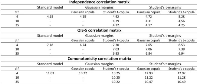
Table 3 shows the different capital requirements obtained with the Standard
Model and Internal Model computations. For the Standard Model we used the inputs and parameters presented in Table 1 and the QIS‐5 line of business correlation matrix.
For the Internal Model we computed the SCR under the four alternative copula‐ based measures of dependence structures. First, we present our results for the Gaussian
margins with the Gaussian copula and, then, with the Student’s t‐copula. Then, we present our results for the Student’s t‐margins with the Gaussian copula, followed by the results with the Student’s t‐copula. All the copulas, including a Student’s t‐distribution, have been considered with4, 10 and 35 degrees of freedom. To establish comparisons within the Internal Model approach, we also examined the independence case, the comonotonicity case and that using the QIS‐5 correlation matrix.
As shown in Table 3, in the case of the independence correlation matrix, the SCR obtained with the Standard Model underestimates the requirements obtained with the Internal Model. However, in the case of the QIS‐5 and comonotonicity correlation matrixes, the SCR obtained with the Standard Model overestimates the requirement obtained with the Internal Model except in cases involving Student’s t‐distribution margins with fewer than ten degrees of freedom and, hence, assuming heavier tails.
Table 3: SCR. Standard Model versus Internal Model
Independence correlation matrix
Standard model Gaussian margins Student’s t‐margins
d.f. Gaussian copula Student’s t‐copula Gaussian copula Student’s t‐copula
4 4.15 4.15 4.62 4.72 5.28
10 ‐ ‐ 4.39 4.31 4.56
35 ‐ ‐ 4.22 4.17 4.25
QIS‐5 correlation matrix
Standard model Gaussian margins Student’s t‐margins
d.f. Gaussian copula Student’s t‐copula Gaussian copula Student’s t‐copula
4 7.18 6.74 7.30 7.65 8.53
10 ‐ ‐ 7.03 7.06 7.38
35 ‐ ‐ 6.83 6.84 6.94
Comonotonicity correlation matrix
Standard model Gaussian margins Student’s t‐margins
d.f. Gaussian copula Student’s t‐copula Gaussian copula Student’s t‐copula
4 11.03 10.22 10.25 12.93 12.92
10 ‐ ‐ 10.25 11.22 11.28
35 ‐ ‐ 10.22 10.47 10.49
Source : Authors’ own. Based on data for the Spanish market 2000 to 2010. Results are expressed in thousands of million Euros
The Standard Model approach provides an SCR estimate of 4.15 thousand million Euros when assuming independence between the lines of business, similar in this respect to the case of the Gaussian copula with Gaussian margins obtained with the Internal
Model. The independence assumption, as expected, invariably provides the smallest value given one particular model, i.e. either the Standard Model or the Internal Model with a copula structure. Correspondingly, the comonotonicity case invariably leads to the highest
SCR estimate with each particular model. In the Standard Model approach, the comonotonicity assumption almost triples the SCR with respect to the requirement obtained under the independence assumption between lines of business, while the QIS‐5 correlation assumption provides an SCR that lies somewhere between the two.
For all the cases considered here, those in which the SCR is calculated with copulas involving Student’s t‐margins produce larger estimates than those obtained with copulas using Gaussian margins. Specifically, the smallest SCR values are obtained when using a Gaussian copula with Gaussian margins with the next smallest being obtained when using the Student’s t‐copula with Gaussian margins. Then, the Gaussian copula with Student’s t‐ margins and the Student’s t‐copula with Student’s t‐margins produce increasingly higher results. Thus, there is evidence that the selection of margins influences the capital calculations and the effect of considering heavy‐tailed marginal distributions becomes noticeable even in the case of the Gaussian copula.
Note also that as the number of degrees of freedom used in the Student’s t‐ margins increases, the SCR obtained for those copulas with Student’s t‐margins decreases compared to margins with a smaller number of degrees of freedom and the results converge to the capital obtained with the Gaussian copula with Gaussian margins. This influence of the number of degrees of freedom was expected and can be observed in all the correlation assumptions, namely, independence, QIS‐5 correlation matrix and comonotonicity.
4
Discussion
Since discussions concerning the Solvency II project were initiated until its eventual adoption by the European Parliament in November 2009, much of the debate centered on the solvency requirements to be imposed on EU insurance companies. The Quantitative
Impact Studies (QIS) undertaken by the regulator tested the impact of implementing the principles contained within Solvency II. Furthermore, since the early stages, participating insurance companies reported their full or partial internal model results so as to provide the regulators with the necessary information to improve the implementation of the Solvency II directives.
Our study seeks to further understanding of the methodology involved in calculating capital requirements. First, drawing on data from the Spanish non‐life underwriting market we have obtained the Solvency Capital Requirement employing the Standard Model approach for the whole market, i.e. as if the market were operating as a single insurance company. This serves market agents, the regulator and Spanish companies alike as a market benchmark tool and insurance companies can compare their own capital estimations with the market position. Regulators can also use the aggregate market calculation to allocate capital to companies and to compare the allocated capital with the capital they are effectively estimating individually. However, we argue that the
Standard Model approach to calculating the non‐life premium and reserve risk sub‐ module is an overly rigid system when using QIS‐5 parameters that depend only on
volume measure. We also believe that this approach does not take into account the premium security margin but rather the underwriting premiums, which could result in wrong conclusions being drawn when comparing two companies with the same premium volumes but different premium security margins.
Second, we have designed an Internal Model approach for calculating the solvency requirement and have compared our results with those obtained employing the standard approach. The first difference to note between the two approaches is the use of the underlying random variable in the Internal Model analysis. We do not consider a mixture of premium and reserve risks by line of business but rather the predicted net result for the forthcoming period by line of business. It is our claim that the latter reflects better the essence of premium and reserve risks. Furthermore, by indicating when there are insufficient resources to cover claims and expenses, positive or negative results are reflected in the profit and loss account. The second difference involves the way in which the capital estimation is arrived at. While the standard approach draws on past data, i.e., last written premium volume by line of business, the internal approach involves predicting the distribution of the net results. It would appear that given the definition of the SCR under Solvency II, this capital requirement should be based on the future evolution of the random variable rather than on its past behavior. Thus we have chosen to base our prediction on the linear regression trend, which provides information regarding the expected path of each random variable, while its prediction error can also be assessed. Finally, the third difference concerns the dependence structure assumptions between lines of business. The standard approach uses correlations of joint parameters by line of business taking a qualitative approach. By contrast, the internal approach uses a Gaussian
copula and Student’s t‐ copula with the same family marginal distributions since the random variables are all defined in real numbers, and we use correlations to join marginals. In this case, the correlations are obtained taking a quantitative approach.
Based on a comparison of the results derived here from the four dependence and distributional assumptions made, we can establish a lowest to highest capital ranking. We observe that, besides copula selection, a key point is the hypothesis regarding margins. The lowest capital requirement is obtained with copulas with Gaussian margins.
Solvency Capital Requirement estimation procedures need to be improved. To achieve this, we believe more disaggregated data are required, since greater frequency and longer time series would increase the overall accuracy of estimations. Furthermore, correlation estimations need to be made using both internal and standard approaches, and here better databases will guarantee better statistical properties for these estimations. It would seem that what is required is a more rigorous analysis of the Standard Model including comparative and sensitivity analyses. These could involve, for instance, an examination of the impact of other parameters, such as dispersion and correlations, focusing on technical as opposed to solely underwriting premiums.
References
Bühlmann, H. and Gisler, A., (2005), A Course in Credibility Theory and its Applications. Springer, ISBN: 3540257535, Berlin.
CEIOPS, (2010); 5th Quantitative Impact Study ‐ Technical Specifications. https://eiopa.europa.eu/consultations/qis/index.html
Demarta, S. and McNeil, A. J., (2005); The t copula and related copulas. International Statistical Review, 73(1), 111‐129.
Embrechts, P., McNeil, A. J. and Frey, R., (2005); Quantitative Risk Management, Concepts, Techniques and Tools. Ed. Princeton University Press, ISBN 0‐691‐12255‐5,
Princeton.
Englund, M., Guillén, M., Gustafsson, J., Nielsen, L. H. and Nielsen, P. J., (2008);
Multivariate Latent Risk: A credibility approach. Astin Bulletin, 38(1), 137‐146.
Filipović, D., (2009); Multilevel Risk Aggregation. Astin Bulletin, 39(2), 565‐575.
Gisler, A., (2009); The insurance risk in the SST and in Solvency II: Modeling and Parameter estimation. ASTIN Colloquium in Helsinki.
Joe, H., (1997); Multivariate Models and Dependence Concepts. Ed. Chapman & Hall, London.
Nelsen, R. B., (1999); An introduction to Copulas. Ed. Springer.
Pfeifer, D. and Straussburger, D, (2008); Stability problems with the SCR aggregation formula. Scandinavian Actuarial Journal, 1, 61‐77.
Savelli, N. and Clemente, G. P., (2009); Modeling aggregate non‐life underwriting risk: standard formula vs internal model. Giornale dell' Instituto degli Attuari,72, 295‐ 333.
Savelli, N. and Clemente, G. P., (2010); Hierarchical structures in the aggregation of premium risk for insurance underwriting. Scandinavian Actuarial Journal, DOI:10.1080/03461231003703672.
Sklar, A., (1959); Fonctions de répartition à n dimensions et leurs marges. Publications de l'Institute de Stadistique de l'Université de Paris, 8, 229‐231.
Sandström, A., (2007); Calibration for skewness. Scandinavian Actuarial Journal, 2, 126‐ 134.
SÈRIE DE DOCUMENTS DE TREBALL DE LA XREAP
2006
CREAP2006-01
Matas, A. (GEAP); Raymond, J.Ll. (GEAP)
"Economic development and changes in car ownership patterns" (Juny 2006)
CREAP2006-02
Trillas, F. (IEB); Montolio, D. (IEB); Duch, N. (IEB)
"Productive efficiency and regulatory reform: The case of Vehicle Inspection Services" (Setembre 2006)
CREAP2006-03
Bel, G. (PPRE-IREA); Fageda, X. (PPRE-IREA)
"Factors explaining local privatization: A meta-regression analysis" (Octubre 2006)
CREAP2006-04
Fernàndez-Villadangos, L. (PPRE-IREA)
"Are two-part tariffs efficient when consumers plan ahead?: An empirical study" (Octubre 2006)
CREAP2006-05
Artís, M. (AQR-IREA); Ramos, R. (AQR-IREA); Suriñach, J. (AQR-IREA) "Job losses, outsourcing and relocation: Empirical evidence using microdata" (Octubre 2006)
CREAP2006-06
Alcañiz, M. (RISC-IREA); Costa, A.; Guillén, M. (RISC-IREA);Luna, C.; Rovira, C.
"Calculation of the variance in surveys of the economic climate” (Novembre 2006)
CREAP2006-07
Albalate, D. (PPRE-IREA)
"Lowering blood alcohol content levels to save lives: The European Experience” (Desembre 2006)
CREAP2006-08
Garrido, A. (IEB); Arqué, P. (IEB)
“The choice of banking firm: Are the interest rate a significant criteria?” (Desembre 2006)
SÈRIE DE DOCUMENTS DE TREBALL DE LA XREAP
CREAP2006-09
Segarra, A. (GRIT); Teruel-Carrizosa, M. (GRIT)
"Productivity growth and competition in spanish manufacturing firms: What has happened in recent years?”
(Desembre 2006)
CREAP2006-10
Andonova, V.; Díaz-Serrano, Luis. (CREB)
"Political institutions and the development of telecommunications” (Desembre 2006)
CREAP2006-11
Raymond, J.L.(GEAP); Roig, J.L.. (GEAP)
"Capital humano: un análisis comparativo Catalunya-España” (Desembre 2006)
CREAP2006-12
Rodríguez, M.(CREB); Stoyanova, A. (CREB)
"Changes in the demand for private medical insurance following a shift in tax incentives” (Desembre 2006)
CREAP2006-13
Royuela, V. (AQR-IREA); Lambiri, D.;Biagi, B.
"Economía urbana y calidad de vida. Una revisión del estado del conocimiento en España” (Desembre 2006)
CREAP2006-14
Camarero, M.; Carrion-i-Silvestre, J.LL. (AQR-IREA).;Tamarit, C.
"New evidence of the real interest rate parity for OECD countries using panel unit root tests with breaks” (Desembre 2006)
CREAP2006-15
Karanassou, M.; Sala, H. (GEAP).;Snower , D. J.
"The macroeconomics of the labor market: Three fundamental views” (Desembre 2006)
SÈRIE DE DOCUMENTS DE TREBALL DE LA XREAP
2007
XREAP2007-01
Castany, L (AQR-IREA); López-Bazo, E. (AQR-IREA).;Moreno , R. (AQR-IREA) "Decomposing differences in total factor productivity across firm size”
(Març 2007)
XREAP2007-02
Raymond, J. Ll. (GEAP); Roig, J. Ll. (GEAP)
“Una propuesta de evaluación de las externalidades de capital humano en la empresa" (Abril 2007)
XREAP2007-03
Durán, J. M. (IEB); Esteller, A. (IEB)
“An empirical analysis of wealth taxation: Equity vs. Tax compliance” (Juny 2007)
XREAP2007-04
Matas, A. (GEAP); Raymond, J.Ll. (GEAP)
“Cross-section data, disequilibrium situations and estimated coefficients: evidence from car ownership demand”
(Juny 2007)
XREAP2007-05
Jofre-Montseny, J. (IEB); Solé-Ollé, A. (IEB)
“Tax differentials and agglomeration economies in intraregional firm location” (Juny 2007)
XREAP2007-06
Álvarez-Albelo, C. (CREB); Hernández-Martín, R.
“Explaining high economic growth in small tourism countries with a dynamic general equilibrium model” (Juliol 2007)
XREAP2007-07
Duch, N. (IEB); Montolio, D. (IEB); Mediavilla, M.
“Evaluating the impact of public subsidies on a firm’s performance: a quasi-experimental approach” (Juliol 2007)
XREAP2007-08
Segarra-Blasco, A. (GRIT)
“Innovation sources and productivity: a quantile regression analysis” (Octubre 2007)
SÈRIE DE DOCUMENTS DE TREBALL DE LA XREAP
XREAP2007-09
Albalate, D. (PPRE-IREA)
“Shifting death to their Alternatives: The case of Toll Motorways” (Octubre 2007)
XREAP2007-10
Segarra-Blasco, A. (GRIT); Garcia-Quevedo, J. (IEB); Teruel-Carrizosa, M. (GRIT) “Barriers to innovation and public policy in catalonia”
(Novembre 2007)
XREAP2007-11
Bel, G. (PPRE-IREA); Foote, J.
“Comparison of recent toll road concession transactions in the United States and France” (Novembre 2007)
XREAP2007-12
Segarra-Blasco, A. (GRIT);
“Innovation, R&D spillovers and productivity: the role of knowledge-intensive services” (Novembre 2007)
XREAP2007-13
Bermúdez Morata, Ll. (RFA-IREA); Guillén Estany, M. (RFA-IREA), Solé Auró, A. (RFA-IREA) “Impacto de la inmigración sobre la esperanza de vida en salud y en discapacidad de la población española”
(Novembre 2007)
XREAP2007-14
Calaeys, P. (AQR-IREA); Ramos, R. (AQR-IREA), Suriñach, J. (AQR-IREA) “Fiscal sustainability across government tiers”
(Desembre 2007)
XREAP2007-15
Sánchez Hugalbe, A. (IEB)
“Influencia de la inmigración en la elección escolar” (Desembre 2007)
SÈRIE DE DOCUMENTS DE TREBALL DE LA XREAP
2008
XREAP2008-01
Durán Weitkamp, C. (GRIT); Martín Bofarull, M. (GRIT) ; Pablo Martí, F.
“Economic effects of road accessibility in the Pyrenees: User perspective” (Gener 2008)
XREAP2008-02
Díaz-Serrano, L.; Stoyanova, A. P. (CREB)
“The Causal Relationship between Individual’s Choice Behavior and Self-Reported Satisfaction: the Case of Residential Mobility in the EU”
(Març 2008)
XREAP2008-03
Matas, A. (GEAP); Raymond, J. L. (GEAP); Roig, J. L. (GEAP) “Car ownership and access to jobs in Spain”
(Abril 2008)
XREAP2008-04
Bel, G. (PPRE-IREA) ; Fageda, X. (PPRE-IREA)
“Privatization and competition in the delivery of local services: An empirical examination of the dual market hypothesis”
(Abril 2008)
XREAP2008-05
Matas, A. (GEAP); Raymond, J. L. (GEAP); Roig, J. L. (GEAP) “Job accessibility and employment probability”
(Maig 2008)
XREAP2008-06
Basher, S. A.; Carrión, J. Ll. (AQR-IREA)
Deconstructing Shocks and Persistence in OECD Real Exchange Rates (Juny 2008)
XREAP2008-07
Sanromá, E. (IEB); Ramos, R. (AQR-IREA); Simón, H.
Portabilidad del capital humano y asimilación de los inmigrantes. Evidencia para España (Juliol 2008)
XREAP2008-08
Basher, S. A.; Carrión, J. Ll. (AQR-IREA)
Price level convergence, purchasing power parity and multiple structural breaks: An application to US cities
(Juliol 2008)
XREAP2008-09
Bermúdez, Ll. (RFA-IREA)
A priori ratemaking using bivariate poisson regression models (Juliol 2008)
SÈRIE DE DOCUMENTS DE TREBALL DE LA XREAP
XREAP2008-10
Solé-Ollé, A. (IEB), Hortas Rico, M. (IEB)
Does urban sprawl increase the costs of providing local public services? Evidence from Spanish municipalities
(Novembre 2008)
XREAP2008-11
Teruel-Carrizosa, M. (GRIT), Segarra-Blasco, A. (GRIT) Immigration and Firm Growth: Evidence from Spanish cities (Novembre 2008)
XREAP2008-12
Duch-Brown, N. (IEB), García-Quevedo, J. (IEB), Montolio, D. (IEB)
Assessing the assignation of public subsidies: Do the experts choose the most efficient R&D projects? (Novembre 2008)
XREAP2008-13
Bilotkach, V., Fageda, X. (PPRE-IREA), Flores-Fillol, R.
Scheduled service versus personal transportation: the role of distance (Desembre 2008)
XREAP2008-14
Albalate, D. (PPRE-IREA), Gel, G. (PPRE-IREA)
Tourism and urban transport: Holding demand pressure under supply constraints (Desembre 2008)
SÈRIE DE DOCUMENTS DE TREBALL DE LA XREAP
2009
XREAP2009-01
Calonge, S. (CREB); Tejada, O.
“A theoretical and practical study on linear reforms of dual taxes” (Febrer 2009)
XREAP2009-02
Albalate, D. (PPRE-IREA); Fernández-Villadangos, L. (PPRE-IREA)
“Exploring Determinants of Urban Motorcycle Accident Severity: The Case of Barcelona” (Març 2009)
XREAP2009-03
Borrell, J. R. (PPRE-IREA); Fernández-Villadangos, L. (PPRE-IREA) “Assessing excess profits from different entry regulations”
(Abril 2009)
XREAP2009-04
Sanromá, E. (IEB); Ramos, R. (AQR-IREA), Simon, H.
“Los salarios de los inmigrantes en el mercado de trabajo español. ¿Importa el origen del capital humano?”
(Abril 2009)
XREAP2009-05
Jiménez, J. L.; Perdiguero, J. (PPRE-IREA)
“(No)competition in the Spanish retailing gasoline market: a variance filter approach” (Maig 2009)
XREAP2009-06
Álvarez-Albelo,C. D. (CREB), Manresa, A. (CREB), Pigem-Vigo, M. (CREB) “International trade as the sole engine of growth for an economy”
(Juny 2009)
XREAP2009-07
Callejón, M. (PPRE-IREA), Ortún V, M.
“The Black Box of Business Dynamics” (Setembre 2009)
XREAP2009-08 Lucena, A. (CREB)
“The antecedents and innovation consequences of organizational search: empirical evidence for Spain” (Octubre 2009)
XREAP2009-09
Domènech Campmajó, L. (PPRE-IREA) “Competition between TV Platforms” (Octubre 2009)
SÈRIE DE DOCUMENTS DE TREBALL DE LA XREAP
XREAP2009-10
Solé-Auró, A. (RFA-IREA),Guillén, M. (RFA-IREA), Crimmins, E. M.
“Health care utilization among immigrants and native-born populations in 11 European countries. Results from the Survey of Health, Ageing and Retirement in Europe”
(Octubre 2009)
XREAP2009-11
Segarra, A. (GRIT), Teruel, M. (GRIT) “Small firms, growth and financial constraints” (Octubre 2009)
XREAP2009-12
Matas, A. (GEAP), Raymond, J.Ll. (GEAP), Ruiz, A. (GEAP) “Traffic forecasts under uncertainty and capacity constraints” (Novembre 2009)
XREAP2009-13 Sole-Ollé, A. (IEB)
“Inter-regional redistribution through infrastructure investment: tactical or programmatic?” (Novembre 2009)
XREAP2009-14
Del Barrio-Castro, T., García-Quevedo, J. (IEB)
“The determinants of university patenting: Do incentives matter?” (Novembre 2009)
XREAP2009-15
Ramos, R. (AQR-IREA), Suriñach, J. (AQR-IREA), Artís, M. (AQR-IREA) “Human capital spillovers, productivity and regional convergence in Spain” (Novembre 2009)
XREAP2009-16
Álvarez-Albelo, C. D. (CREB), Hernández-Martín, R.
“The commons and anti-commons problems in the tourism economy” (Desembre 2009)