c
DEEP GENERATIVE MODELS VIA EXPLICIT WASSERSTEIN MINIMIZATION
BY
YUCHENG CHEN
THESIS
Submitted in partial fulfillment of the requirements for the degree of Master of Science in Computer Science
in the Graduate College of the
University of Illinois at Urbana-Champaign, 2019
Urbana, Illinois Adviser:
ABSTRACT
This thesis provides a procedure to fit generative networks to target distributions, with the goal of a small Wasserstein distance (or other optimal transport costs). The approach is based on two principles: (a) if the source randomness of the network is a continuous distribution (the “semi-discrete” setting), then the Wasserstein distance is realized by a deterministic optimal transport mapping; (b) given an optimal transport mapping between a generator network and a target distribution, the Wasserstein distance may be decreased via a regression between the generated data and the mapped target points. The procedure here therefore alternates these two steps, forming an optimal transport and regressing against it, gradually adjusting the generator network towards the target distribution. Mathematically, this approach is shown to minimize the Wasserstein distance to both the empirical target distribution, and also its underlying population counterpart. Empirically, good performance is demonstrated on the training and testing sets of the MNIST and Thin-8 data. As a side product, the thesis proposes several effective metrics of measure performance of deep generative models. The thesis closes with a discussion of the unsuitability of the Wasserstein distance for certain tasks, as has been identified in prior work.
ACKNOWLEDGMENTS
I would like to thank my advisor Professor Jian Peng for his enduring support and guid-ance. I would also like to thank my other collaborators Professor Matus Telgarsky, Professor Chao Zhang, Professor Daniel Hsu, and Bolton Bailey, especially Professor Telgarsky who have contributed to many original results presented in the thesis. I would like to thank Professor Jiawei Han for the great opportunities and advice he provided to me. I would also like to thank Dr. Xing Xie, Dr. Jing Yuan, Yuqing Zhu, and Dr. Hao Zhang for their support and help during my precious experience of internships. Special thanks to Viveka Kudaligama, Maggie Metzger Chappell and Kathy Runck for their excellent work which greatly helped my student life and thesis. Finally, I would like to thank my wife Shan Jiang for her advice and support in both academics and life.
TABLE OF CONTENTS
CHAPTER 1 INTRODUCTION . . . 1
CHAPTER 2 REVIEW OF RELATED WORKS . . . 6
2.1 Optimal Transport . . . 6
2.2 Deep Generative Models . . . 6
2.3 Evaluation of DGMs . . . 8
2.4 Generalization Properties of Wasserstein Distance . . . 9
CHAPTER 3 THE OPTIMAL-TRANSPORT SOLVER . . . 10
3.1 Preliminaries: Optimal Transport . . . 10
3.2 The Semi-Discrete Optimal-Transport Solver (OTS) . . . 11
3.3 Acceleration via Subsampling . . . 14
CHAPTER 4 THE GENERATOR FITTING ALGORITHM . . . 17
4.1 The Fitting Step (FIT) . . . 17
4.2 The Overall Algorithm . . . 18
CHAPTER 5 THEORETICAL ANALYSIS . . . 19
5.1 Optimization Guarantee . . . 19
5.2 Generalization Guarantee . . . 20
5.3 Verifying the Generalization Assumption . . . 22
CHAPTER 6 EXPERIMENTAL RESULTS . . . 23
6.1 Experimental Setup . . . 23
6.2 Qualitative Study . . . 26
6.3 Quantitative Results . . . 29
CHAPTER 7 EVALUATION OF GANS . . . 33
7.1 Defining New Metrics . . . 33
7.2 Evaluation Results . . . 35
CHAPTER 8 DISCUSSION ON LIMITATIONS . . . 38
CHAPTER 9 CONCLUSION . . . 42
CHAPTER 1: INTRODUCTION
Deep generative models (DGMs), which are deep neural networks modeling complex dis-tributions by first sampling from simple disdis-tributions such as multivariate Gaussian, and then transforming the samples to complex targets such as images, has become increasing popular and successful in various real-world applications such as image synthesis [1], style transfer [2], and music generation [3].
Generative Adversarial Networks (GANs) [4] is arguably the most successful family of DGMs in recent years. GANs optimize both the generator network, as well as a second discriminator or adversarial network: first the discriminator was fixed and the generator was optimized to fool it, and second the generator was fixed and the discriminator was optimized to distinguish it from real samples. This procedure was originally constructed to minimize a Jensen-Shannon Divergence via a game-theoretic derivation. Subsequent work derived the adversarial relationship in other ways, for instance the Wasserstein GAN used duality properties of the Wasserstein distance [5].
Despite its huge success, GAN suffers from two well-known limitations. First, the adver-sarial training process is unstable and prone to mode-collapse. Second, since the Jensen-Shannon or Wasserstein divergences is not optimized explicitly but instead indirectly by neural-network approximation and game-theoretic process, it is not clear that how such di-vergences are actually minimized, and it is also not clear how to quantitatively evaluate the closeness between generated and target distributions. In practice, careful hyper-parameter tuning and various tricks may prevent such issues from serious affecting the results, but this would usually require a large number of trial-and-errors before success.
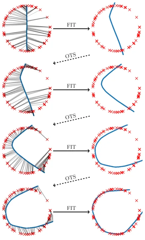
In this thesis, we attempt to alleviate such limitations of GANs by proposing a simple non-adversarial but still alternating procedure to fit generative networks to target distributions. The procedure explicitly optimizes the Wasserstein-p distance between the generator g#µ and the target distribution ˆν. As depicted in Figure 1.1, it alternates two steps: given a current generator gi, an Optimal Transport Solver (OTS) associates (or “labels”) gi’s
probability mass with that of the target distribution ˆν, and then a fitting procedure (FIT) uses this labeling to find a new generator gi+1 via a standard regression.
FIT OTS FIT OTS FIT OTS FIT
Figure 1.1: The goal in this example is to fit the initial distribution (the blue central line) to the target distribution (the red outer ring). The algorithm alternates OTS and FIT steps, first (OTS) associating the input distribution samples with target distribution samples, and secondly (FIT) shifting input samples towards their targets, thereafter repeating the process. Thanks to being gradual, and not merely sticking to the first or second OTS, the process has a hope of constructing a simple generator which generalizes well.
The effectiveness of this procedure hinges upon two key properties: it is semi-discrete, meaning the generators always give rise to continuous distributions, and it isgradual, mean-ing the generator is slowly shifted towards the target distribution. The key consequence of being semi-discrete is that the underlying optimal transport can be realized with a de-terministic mapping. Solvers exist for this problem and construct a transport between the continuous distribution g#µ and the target ˆν; by contrast, methods forming only batch-to-batch transports using samples from g#µ are biased and do not exactly minimize the Wasserstein distance [6, 7, 8, 9].
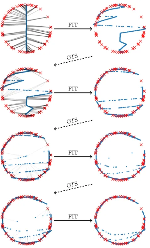
The procedure also aims to be gradual, as in Figure 1.1, slowly deforming the source distribution into the target distribution. While it is not explicitly shown that this gradual property guarantees a simple generator, promising empirical results measuring Wasserstein distanceto a test set suggest that the learned generators generalize well. Figure 1.2 gives an example similar to Figure 1.1, except that FIT step will iterate itself until stuck at a local optimum. The learned manifold after the first step is a zig-zag shaped curve which does not generalize. While the alternating procedure is able to further push the generated samples to targets, the learned manifold is not as smooth as in Figure 1.1.
We show that our proposed method has a variety of theoretical guarantees Foremost amongst these are showing that the Wasserstein distance is indeed minimized, and secondly that it is minimized with respect to not just the dataset distribution ˆν, but moreover the underlying ν from which ˆν was sampled. This latter property can be proved via the triangle inequality for Wasserstein distances, however such an approach introduces the Wasserstein distance between νand ˆν, namely W(ν,ν), which is exponential in dimension even in simpleˆ cases [10, 11, 12]. Instead, we show that when a parametric model captures the distributions well, then bounds which are polynomial in dimension are possible.
Empirically, we find that our method generates both quantitatively and qualitatively bet-ter digits than the compared baselines on MNIST, and the performance is consistent on both training and test datasets. We also experiment with the Thin-8 dataset [12], which is considered challenging for methods without a parametric loss.
As a side result of our method, OTS is able to measure the Wasserstein-pdistance between generated and target distribution, which makes it capable as an evaluation tool of DGMs. We apply our tool to GAN [4], LSGAN [13], WGAN [5] and WGAN-GP [14] with different generator and discriminator architectures.
The rest of the thesis is structured as follows. In Chapter 2, we review the previous works in deep generative models, evaluation methods, and optimal transport. In Chapter 3, we introduce preliminaries of optimal transportation theory, then propose our semi-discrete optimal-transport solver, along with methods to accelerate its computation. In Chapter 4,
we first present our fitting procedure, and then the overall generator training algorithm. In Chapter 5, we give theoretical analysis of the optimization and generalization properties of our method. In Chapter 7, we briefly describe how to use our method to evaluate deep generative models. In Chapter 6, we present our experimental results both qualitatively and quantitatively, and also presents evaluation results of a variety of GAN methods. In Chapter 8 and Chapter 9, we discuss the limitations of our method and conclude with some future directions.
FIT OTS FIT OTS FIT OTS FIT
CHAPTER 2: REVIEW OF RELATED WORKS
2.1 OPTIMAL TRANSPORT
Optimal transport, which is to find optimal plans to move between probability measures, is an old yet vibrant topic. Two classic reference books of optimal transport are [15] and [16], and the recent book [17] gives a comprehensive introduction to modern optimal transport algorithms, with an emphasis on computational methods.
By continuity of input distributions, optimal tranport algorithms can be classified into the following 3 classes: discrete OT, semi-discrete OT and continuous OT. For the task of evaluating and training generative models, semi-discrete OT is of particular interest, since the generated images G(z) forms a continuous distribution while the training and test datasets are discrete. [18] provides a geometric view of semi-discrete optimal transport.
Comparing to traditional optimal transport algorithms applying linear programming or network flow, it is found that stochastic algorithms based on dual formulation of optimal transport achieves faster convergence, and can be naturally extended to semi-discrete and continuous formulations [19]. In [19], the dual variables (a.k.a. Kantorovich potential) is extended to continuous space via reproducing kernel Hilbert spaces. On the other hand, [20] achieves the same goal by parameterizing the Kantorovich potential via neural networks. Most stochastic optimization algorithms in [19] and [20] imposes an entropic regularization to the optimal transport formulation: it has many advantages, for example guarantee of unique optimal solution, faster algorithms [21] with Sinkhorn algorithm [22], etc.
On the other hand, in our context one would like to exactly compute Wasserstein metric without any regularization to obtain an accurate measurement of generator performance. Our work will focus on non-regularized semi-discrete optimal transport, and its application on evaluation and training of GANs.
2.2 DEEP GENERATIVE MODELS
In recent years there has been a huge amount of research interest in the area of deep generative models. We first briefly survey the two most popular families of DGMs: generative adversarial networks (GANs) andvariational auto-encoders (VAEs), then focus on discussing works on the joint field of DGMs and optimal transport, as they have closer relationship to our work.
the perspective of auto-encoders (AEs), VAEs can be alternatively viewed as a regularized form of AEs, where reconstruction error and prior restriction to latent codes are jointly optimized. [24] serves as a comprehensive tutorial to VAEs.
Generative Adversarial Networks [4] train both the generator and a separate discriminator in an adversarial way: the discriminator is trained to distinguish between real and gener-ated samples, and the generator is trained to fool the discriminator. The original training objective of GANs is equivalent to minimizing a lower bound on the Jensen-Shannon diver-gence of the generated and target distributions, and a slight variant of the original objective is equivalent to minimizing a lower bound on their KL-divergence. Both objectives suffers from vanishing gradient [25] which motivates development of Wasserstein GANs (WGAN) [5].
Lots of works have appeared recently on the joint area of optimal transport and generative modeling, WGAN [5] and its variant WGAN-GP [14] approximate Wasserstein-1 distance as their training target, by applying Kantorovich-Rubinstein duality ([15], Theorem 1.14):
W(µ, ν) = sup Lip(f)≤1
Ex∼µf(x)−Ex∼νf(x) (2.1)
Lip(f) ≤ 1 is approximated by the function class of neural networks. In WGAN, the weights of the neural networks are restricted, in order to bound the Lipschitz constant of neural networks, while in WGAN-GP the weights are unrestricted, but a regularization on gradients at the interlopations between samples is introduced.
Wasserstein auto-encoder (WAE) ([26], [27]) optimizes Wasserstein distance by introduc-ing a relaxation to its primal form. [28] gives a comparison of WGAN and WAE from the view of optimal transportation theory.
The idea of computing optimal transport between batches of generated and real sam-ples has been used in both non-adversarial generative modeling [7, 29], as well as adversarial generative modeling [8, 9]. [7] optimizes an interpolation of regularized OT and MMD (max-imum mean discrepancy) losses. [29] compute discrete OT with proximal point methods and extend to generative models. [8] propose a variant to GAN which minimizes a combination of optimal transport and energy distance. [9] proposes a neural-approximated form and incor-porate it into the formulation of WGAN. Nonetheless, minimizing batch-to-batch transport distance does not lead to the minimization of the Wasserstein distance between the gener-ated and target distributions [6]. Instead, our method computes the whole-to-whole optimal transport via the semi-discrete formulation.
[20] proposes to train generative networks by fitting towards the optimal transport plan between latent code and data, which can be considered as a special case of the non-alternating
procedure we discussed earlier. Important limitations of the method in [20] includes requiring latent code having the same dimension as data, and not directly optimizing any distance between generated and target distributions.
2.3 EVALUATION OF DGMS
The most important reason that generative adversarial networks [4] becomes extremely popular is probably that it can generate images with unprecedented quality. However, eval-uating the quality of generative models is still a diffcult task and perhaps no silver bullet would exist for every application, as surveyed and discussed in [30] and [31].
[32] critically surveys popular evaluation metrics for GANs. Inception score [33] is proba-bly the most popular evaluation metrics in the GAN literature, with several variants proposed [34, 35]. It favors models that generate easy-to-classify samples by an external classification model, and with diverse class distribution. While being widely accepted and reasonably correlated to human perception of images, inception score and its variants have certain lim-itations. Relying an external model, inception score does not directly measures how the generators learn from their training data, but instead measures how they generate samples favored by the inception model. Also, diversity of labels does not guaranttee removal of mode collapse, which will be demonstrated by experimental results in our work.
Another line of GAN evaluation metrics attempts to measure distance between distribu-tion of generated samples and distribudistribu-tion of real data. Such distance measures include Wasserstein metric [5], Fr´echet Inception Distance [36], maximum mean discrepancy [37, 38] and so on. [39] performs empirical study using FID under a large-scale search of hyperpa-rameters.
Our work will focus on Wasserstein metric, which is widely used both for training [5, 14] and evaluating [40, 41] GANs. Instead of exactly computing Wasserstein distance, and the supremum over all Lipschitz-1 functions is substituted by that over a function class of neural networks, with weight clippling or gradient penalty. It is still unknown how good these workarounds are. In contrast, we aim to evaluate GAN models by exactly compute the Wasserstein distance between generated images and training datasets through stochastic optimal transport algorithms.
On quantitatively measuring mode collapse, [42] proposes using birthday paradox test to estimate the support size of generated samples. [43] constructs datasets with known modes for counting number of modes covered.
2.4 GENERALIZATION PROPERTIES OF WASSERSTEIN DISTANCE
[10] analyzes the sample complexity of evaluating integral probability metrics. [11] shows that KL-divergence and Wasserstein distances do not generalize well in high dimensions, but their neural net distance counterparts do generalize. [12] gives reasons for the advantage of GAN over VAE, and collects the Thin-8 dataset to demonstrate the advantage of GANs, which is used in our experiments.
The previous works focus on the worst case where exponential number of samples (w.r.t. dimensionality) is required. On the other hand, our work proposes that there are provable and verifiable cases that polynomial number of samples is sufficient. We will compare both our theoretical and empirical findings with those in [11, 12].
CHAPTER 3: THE OPTIMAL-TRANSPORT SOLVER
3.1 PRELIMINARIES: OPTIMAL TRANSPORT
Given two vector spaces X and Y denoting the origin and destination of masses respec-tively, and a cost function c : X×Y → R, where c(x, y) is the cost of moving x ∈ X to y ∈ Y. In the context of generative modeling, X and Y are usually the same space (the space of generated and target samples), and c(x, y) is a metric defined forx, y ∈X.
Given two probability measures (distributions) µ on X and ν on Y. For a deterministic mapping T between X and Y, we define the distribution of T(x)∈Y where x∼µasT#µ, where # is called the pushforward operator. The Monge optimal transportation problem is defined as finding a deterministic mapping T :X →Y such that T#µ=ν, and theoptimal transport cost Tc(µ, ν) := inf T#µ=ν Z X c(x, T(x))dµ (3.1) is achieved. We call T as a Monge optimal transference plan. y = T(x) denotes that x is “transported” to y by the plan T, with the cost of c(x, y).
In some cases, we would like the mass in somex∈X be split and transported to multiple y ∈ Y. Mass is allowed to split because sometime it is necessary (for example, when µ is a point mass on X), and also for computational reasons. Formally, define coupling Π(µ, ν) as the collection of measures on X ×Y with marginal distributions µ and ν. We define Kantorovich optimal transportation problem as finding a coupling measure π ∈Π(µ, ν) such that the optimal transportation cost
OT(µ, ν) := inf
π∈Π(µ,ν) Z
X×Y
c(x, y)dπ (3.2)
is achieved. π is called as a Kantorovich optimal transference plan. Throughout the thesis we will use the notation Tc for both Monge and Kantorovich optimal transport cost: there
will be no ambiguity wherever we use it.
Now we give an informal derivation of the Kantorovich duality on which our method heavily relies. See Chapter 1 of [15] for the rigorous proof. Define Kantorovich potentials ϕ(x), ψ(y) on X, Y respectively, along with the following optimization problem
I(π) := sup ϕ∈L1(dµ),ψ∈L1(dν) Z X ϕ(x)dµ+ Z Y ψ(y)dν− Z X×Y (ϕ(x) +ψ(y)) dπ (3.3) where L1(dµ) is the class of dµ-almost absolutely integratable functions.
It is easy to verify that if π ∈ Π(µ, ν), then I(π) = 0; otherwise, I(π) = +∞, as we can give ϕ(x) and ψ(y) arbitrarily large values on (x, y) within the discrepancies between the (µ, ν) and the marginal distributions of π.
Then, the infimum over Π(µ, ν) can be rewritten as infimum over arbitrary distribution onX×Y with I(π) as an indicator operator:
Tc(µ, ν) = inf π supϕ,ψ Z X×Y c(x, y)dπ+ Z X ϕ(x)dµ+ Z Y ψ(y)dν− Z X×Y (ϕ(x) +ψ(y)) dπ = inf π supϕ,ψ Z X ϕ(x)dµ+ Z Y ψ(y)dν− Z X×Y (ϕ(x) +ψ(y)−c(x, y)) dπ = sup ϕ,ψ inf π Z X ϕ(x)dµ+ Z Y ψ(y)dν− Z X×Y (ϕ(x) +ψ(y)−c(x, y)) dπ (3.4) where minimax principle is applied for the last equality.
If for any non-zero measure subset ofX×Y, ϕ(x) +ψ(y)> c(x, y), then π can be chosen so that
Z
X×Y
(ϕ(x) +ψ(y)−c(x, y))
can be arbitrary large, and the infimum equals to −∞. Therefore, the supremum has to be taken over Φc, the collection of pairs of (ϕ, ψ) where ϕ ∈ L1(dµ), ψ ∈ L1(dν) and ϕ(x) +ψ(y)≤c(x, y) for dµ-almostx and dν-almosty.
In this case, the infimum overπ is achieved at π= 0 and Tc(µ, ν) = sup (ϕ,ψ)∈Φc Z X ϕ(x)dν+ Z Y ψ(y)dν (3.5)
which is called the Kantorovich dual form of optimal transport.
3.2 THE SEMI-DISCRETE OPTIMAL-TRANSPORT SOLVER (OTS)
To apply optimal transport to our generative modeling case, we first discuss several unique properties of our problem, comparing to the general optimal transport formulation discussed in Section 3.1. First, we would like to compute the optimal transport cost between the distributions of generated samples and real samples, which come from the same space. We use X to denote this space. A popular choice of optimal-transport-based distance notion is the Wasserstein-p metric:
Wp(µ, ν) := inf π∈Π(µ,ν) Z X d(x, y)pdπ 1/p , (3.6)
where d is a metric (a usual choice is the`q metric) on X. Wp(µ, ν) equals to the 1/p power
of the Kantorovich optimal transport cost with cost function c(x, y) := d(x, y)p.
Second, the generated samples has the formg(z) where z is usually drawn from a simple distribution e.g. standard multivariate Gaussian. We useµto denote the simple distribution and the generated distribution is g#µ.
Finally, the the target distribution ν = ˆν is an empirical measure, meaning the uniform distribution on a training set {y1, ..., yN}. Wheng#µ is continuous, the optimal transport
problem here becomes semi-discrete, and the maximizing choice of ϕcan be solved analyti-cally, transforming the problem to optimization over a vector in RN:
Tp(g#µ,ν) = supˆ ϕ,ψ∈Φc Z X ϕ(x)dg#µ(x) + 1 N N X i=1 ψ(yi) = sup ϕ∈Φ0 c,ψˆ, ˆ ψ∈RN Z X ϕ(x)dg#µ(x) + 1 N N X i=1 ˆ ψi = sup ˆ ψ∈RN Z X min i (c(x, yi)− ˆ ψi)dg#µ(x) + 1 N N X i=1 ˆ ψi, (3.7)
where ˆψi :=ψ(yi), and Φ0c,ψˆ is the collection of functions ϕ∈L1(d(g#µ)) such thatϕ(x) + ˆ
ψi ≤c(x, yi) for almost allxandi= 1, ..., N. The third equality comes from the maximizing
choice of ϕ: ϕ(x) = mini(c(x, yi)−ψˆi).
Our OTS solver, presented in Algorithm 3.1, uses SGD to maximize eq. (3.7), or rather to minimize its negation
− Z X min i (c(x, yi)− ˆ ψi)dg#µ(x)− 1 N N X i=1 ˆ ψi. (3.8)
OTS is similar to Algorithm 2 of [19], but without averaging. Note as follows that Algo-rithm 3.1 is convex in ˆψ, and thus a convergence theory of OTS could be developed, although this direction is not pursued here.
Algorithm 3.1 Optimal Transport Solver (OTS)
Input: continuous generated distributiong#µ, training dataset (y1, ..., yn) corresponding
to ˆν, cost function c, batch size B, learning rate η. Output: ψˆ= ( ˆψ1, ...,ψˆN)
Initializet := 0 and ˆψ(0) ∈
RN.
repeat
Generate samples x= (x1, ..., xB) from g#µ.
Define loss l(x) := B1 PB j=1mini(c(xj, yi)−ψˆi) + N1 PN i=1ψˆi. Update ˆψ(t+1) := ˆψ(t)+η· ∇ ˆ ψl(x). Update t:=t+ 1.
untilStopping criterion is satisfied. return ψˆ(t).
Proposition 3.1. Equation (3.8) is a convex function of ψˆ. Proof. It suffices to note that mini
c(g(x), yi)−ψˆi
is a minimum of concave functions and thus concave; eq. (3.8) is therefore concave since it is a convex combination of concave functions with an additional linear term.
Note that the optimal transport cost computed via Equation (3.5) is the cost for the Kantorovich optimal transference plan, where mass can be split, which is a relaxation of the Monge optimal transference plan, where mass cannot be split and a deterministic mapping T exists between x∼µ0 and y∼ν0, as discussed in Section 3.1.
A deterministic Monge OT mapping is crucial to our setup, since it provides the regression target for our FIT step. In general, Monge and Kantorovich OT plans are different; in our semi-discrete setting, the Kantorovich OT plan is unique and does not split mass, making it also a Monge OT plan, assuming the cost function is strictly convex and superlinear ([15], Theorem 2.44):
Proposition 3.2. Assume X =Rd, g#µ is continuous, and the cost function c(x, y) takes
the form of c(x−y) and is a strictly convex, superlinear function on Rd. Given the optimal
ˆ
ψ for eq. (3.8), then T(x) := arg minyic(x, yi)−ψˆi, which is a Monge transference plan, is
Proof. By Theorem 2.44 of [15], if T(x) can be uniquely determined by T(x) = x − ∇c∗(∇ϕ(x)), where ϕ is defined in eq. (3.5), then T(x) is the unique Monge-Kantorovich
optimal transference plan. Defining m := arg minic(x−yi)−ψˆi for convenience, we have
T(x) =x− ∇c∗(∇ϕ(x)) =⇒ x−T(x) =∇c∗(∇ϕ(x)) =∇c∗(∇xmin i c(x−yi)− ˆ ψi) =∇c∗∇x(c(x−ym)−ψˆm) =∇c∗∇c(x−ym) =x−ym =⇒ T(x) =ym = arg min yi c(x−yi)−ψˆi
which concludes the proof. Some remarks:
1. We use arg minyic(x, yi)−ψˆi for yarg minic(x,yi)−ψˆi as a slight abuse of notation.
2. Wasserstein-p distances on `p metric with p > 1 satisfy strict convexity and
super-linearity, while p = 1 does not. On the other hand, in practice we have found that for p = 1, Algorithm 3.1 still converges to near-optimal transference plans, and this particular choice of metric generates crispier images than others.
3. The continuity of g#µ, which is required for the existence of Monge transference plan, holds ifg is a feedforward neural network with non-degenerate weights, and invertible activation function such as sigmoid, tanh, or leaky ReLU. For non-invertible activation function such as ReLU, it is possible that g#µgives mass to a discrete subset of Rd;
however, this did not happen in our experiments, and moreover can be circumvented by adding a small perturbation to g’s output. It is possible to prove an extension of Theorem 2.44 of [15] under milder assumptions: we hope to explore this direction in the future.
3.3 ACCELERATION VIA SUBSAMPLING
A drawback of Algorithm 3.1 is that computing minimum on the whole dataset hasO(N) complexity, which is costly for extremely large datasets. For moderately sized datasets such
as MNIST, the efficiency is acceptable, as will be presented in Chapter 6, but it might be prohibitive for very large datasets.
This motivates us to find a solution that can avoid computing max over the whole dataset. Our solution turns out to be very simple: for every iteration, we only sample a portion of dataset y, compute max over the sampled y’s, and then update their ˆψ, as detailed in Algorithm 3.2.
Algorithm 3.2 Optimal Transport Solver (OTS)
Input: continuous generated distributiong#µ, training dataset (y1, ..., yn) corresponding
to ˆν, cost function c, batch size B, subsample size C, learning rate η. Output: ψˆ= ( ˆψ1, ...,ψˆN)
Initializet := 0 and ˆψ(0) ∈RN.
repeat
Generate samples x= (x1, ..., xB) from g#µ.
Draw s1, ..., sC uniformly from{1, ..., N}.
Define loss l(x) := B1 PB j=1mini(c(xj, ysi)−ψˆsi) + 1 C PC i=1ψˆsi. Update ˆψ(t+1) := ˆψ(t)+η· ∇ ˆ ψl(x). Update t:=t+ 1.
untilStopping criterion is satisfied. return ψˆ(t).
To intuitively see how Algorithm 3.2 works, let us take a look on how SGD is performed in Algorithm 3.1 more closely. For each iteration, a batch ofxis sampled and −c(xi, yj)−ψˆj
is computed for each yj, and a batch of arg maxyj−(xi, yj)−
ˆ
ψj are obtained. Then those
“arg max ˆψj” are penalized by SGD (by decreasing all the other ˆψj), making them less likely
to be argmax again. In Algorithm 3.2, argmax of a subsample of y is selected and then penalized. If the maximum over the subsample is not far away it over the whole dataset, then we could expect this subsample maximum to be penalized later by Algorithm 3.1, and Algorithm 3.2 does this penalization early for faster convergence.
Mathematically, Algorithm 3.1 optimizes f( ˆψ) := Eµmax j −c(x, yj)−ψˆj + 1 n n X j=1 ˆ ψj (3.9)
while Algorithm 3.2 optimizes fs( ˆψ) := Es Eµmax sj −c(x, ysj)−ψˆsj + 1 C C X j=1 ˆ ψsj ! (3.10)
whereEs:=Es1,...,sC∈{1,...,n}. Under mild assumptions of data, the difference between eq. (3.9)
CHAPTER 4: THE GENERATOR FITTING ALGORITHM
4.1 THE FITTING STEP (FIT)
Given an initial generator g, and an optimal transference plan T between g#µ and ˆν thanks to OTS, we update g to obtain a new generator g0 by simply sampling z ∼ µ and regressing the new generated sample g0(z) towards the old OT plan T(g(z)), as detailed in Algorithm 4.1.
Under a few assumptions detailed in Section 5.1, Algorithm 4.1 is guaranteed to return a generator g0 with strictly lesser optimal transport cost
Tc(g0#µ,ν)ˆ ≤Ex∼g0#µc(x, T(x))<Ex∼g#µc(x, T(x)) = Tc(g#µ,ν),ˆ (4.1) whereT denotes an exact optimal plan between g#µ and ˆν; Section 5.1 moreover considers the case of a merely approximately optimal T, as returned by OTS.
Algorithm 4.1 Fitting Optimal Transport Plan (FIT)
Input: sampling distribution µ, old generator g with parameter θ, transference plan T, cost function c, batch size B, learning rate η.
Output: new generator g0 with parameter θ0. Initializet := 0 and g0 with parameter θ0(0) =θ. repeat
Generate random noise z= (z1, ..., zB) from µ.
Define loss l(z) := B1 PB j=1c(g 0(z), T(g(z))). Update θ(t+1) :=θ0(t)−η· ∇ θ0l(z). Update t:=t+ 1.
untilStopping criterion is satisfied. return g0 with parameter θ0(t).
4.2 THE OVERALL ALGORITHM
The overall algorithm, presented in Algorithm 4.2, alternates between OTS and FIT: dur-ing iterationi, OTS solves for the optimal transport map T between old generated distribu-tion gi#µ and ˆν, then FIT regresses gi+1#µ towards T#gi#µ to obtain lower Wasserstein
distance.
Algorithm 4.2 Overall Algorithm
Input: sampling distributionµ, training dataset (y1, ..., yn) corresponding to ˆν, initialized
generator g0 with parameter θ0, cost function c, batch size B, learning rate η. Output: final generator g with parameter θ.
Initializei:= 0 and g0 with parameter θ(0) =θ0. repeat
Compute ˆψi := OTS(gi#µ,ν, c, B, η).ˆ
Get Ti asTi(x) := arg minyic(x, yi)−
ˆ ψi.
Compute gi+1 := FIT(µ, gi, Ti, c, B, η) with parameterθ(i+1).
Update i:=i+ 1.
untilStopping criterion is satisfied. return g with parameter θ(i).
CHAPTER 5: THEORETICAL ANALYSIS
We now analyze the optimization and generalization properties of our Algorithm 4.2: we will show that the method indeed minimizes the empirical transport cost, meaning Tc(gi#µ,ν)ˆ → 0, and also generalizes to the transport cost over the underlying
distribu-tion, meaning Tc(gi#µ, ν)→0.
5.1 OPTIMIZATION GUARANTEE
Our analysis works for general transportation costsTc that satisfy the triangle inequality,
which holds for Wasserstein-p distances over any metric space, if p≥1 ([15], Theorem 7.3). Our method is parameterized by a scalarα∈(0,1/2) whose role is to determine the relative precisions of OTS and FIT, controlling the gradual property of our method. We assume that for each round i, there exist error terms ot1, ot2, fit such that:
1. Round i of OTS finds transportTi satisfying
Tc(gi#µ,ν)ˆ ≤
Z
c(Ti◦gi, gi)dµ≤ Tc(gi#µ,ν)(1 +ˆ ot1), (approximate optimality)
Tc(Ti#gi#µ,ν)ˆ ≤ot2≤αTc(gi#µ,ν);ˆ (approximate pushforward)
2. Round i of FIT findsgi+1 satisfying Z c(Ti◦gi, gi+1)dµ≤fit ≤ 1−2α 1 +ot1 Z c(Ti◦gi, gi)dµ≤(1−2α)Tc(gi#µ,ν)ˆ (progress of FIT);
3. Each gi#µis continuous (continuity of generation).
The first assumption is satisfied by Algorithm 3.1 since it represents a convex problem; moreover, it is necessary in practice to assume only approximate solutions. The second assumption holds when there is still room for the generative network to improve Wasserstein distance: otherwise, the training process can be stopped. The third assumption is satisfied in general conditions as discussed in Proposition 3.2.
α is a tunable parameter of our overall algorithm: a large α relaxes the optimality re-quirement of OTS (which allows early stopping of Algorithm 3.1) but requires large progress
of FIT (which prevents early stopping of Algorithm 4.1), and vice versa. This gives us a principled way to determine the stopping criteria of OTS and FIT.
Given the assumptions, we now showTc(gi#µ,ν)ˆ →0. By triangle inequality,
Tc(gi+1#µ,ν)ˆ ≤ Tc(gi+1#µ, Ti#gi#µ) +Tc(Ti#gi#µ,ν)ˆ ≤ Tc(gi+1#µ, Ti#gi#µ) +ot2. Sincegi+1#µis continuous, Tc(gi+1#µ, Ti#gi#µ) is realized by some deterministic
trans-port Ti0 satisfying Ti0#gi+1#µ=Ti#gi#µ, whereby
Tc(gi+1#µ, Ti#gi#µ) =
Z
c(Ti0◦gi+1, gi+1)dµ= Z
c(Ti◦gi, gi+1)dµ≤fit. Combining these steps with the upper bounds on ot2 and fit,
Tc(gi+1#µ,ν)ˆ ≤ot2+fit≤(1−α)Tc(gi#µ,ν)ˆ ≤e−αTc(gi#µ,ν).ˆ
Summarizing these steps and iterating this inequality gives the following bound onTc(gt#µ,ν),ˆ
which goes to 0 as t→0.
Theorem 5.1. Suppose (as discussed above) that Tc satisfies the triangle inequality, each
gi#µ is continuous, and the OTS and FIT iterations satisfy
Tc(Ti#gi,#µ,ν)ˆ ≤ot2≤αTc(gi#µ,ν),ˆ (5.1)
Z
c(Ti◦gi, gi+1)dµ≤fit ≤(1−2α)Tc(gi#µ,ν).ˆ (5.2)
Then Tc(gt#µ,ν)ˆ ≤e−tαTc(g0#µ,ν)ˆ .
5.2 GENERALIZATION GUARANTEE
In the context of generative modeling, generalization means that the model fitted via training dataset ˆν not only has low divergence D(gi#µ,ν) to ˆˆ ν, but also low divergence to
ν, the underlying distribution from which ˆν is drawn i.i.d.. If Tc satisfies triangle inequality,
then
Tc(gi#µ, ν)≤ Tc(gi#µ,ν) +ˆ Tc(ˆν, ν), (5.3)
and the second term goes to 0 with sample sizen → ∞, but the sample complexity depends exponentially on the dimensionality [10, 11, 12]. To remove this exponential dependence, we make parametric assumptions about the underlying distribution ν; a related idea was
investigated in detail in parallel work [44].
Our approach is to assume the Kantorovich potential ψ, defined on ˆˆ ν, is induced from a function ψ ∈ Ψ defined on ν, where Ψ is a function class with certain approximation and generalization guarantees. Since neural networks are one such function classes (as will be discussed later), this is an empirically verifiable assumption (by fitting a neural network to approximate ˆψ), and is indeed verified in the Appendix.
For this part we use slightly different notation: for a fixed sample size n, let (gn, Tn,νˆn)
denote the earlier (g, T,ν). We first suppose the followingˆ approximation condition: Suppose that for any >0, there exists a class of functions Ψ so that
sup ψ∈L1(ν) Z ψcdµ+ Z ψdν ≤+ sup ψ∈Ψ Z ψcdµ+ Z ψdν; (5.4)
thanks to the extensive literature on function approximation with neural networks [45, 46, 47], there are various ways to guarantee this, for example increasing the depth of the network. A second assumption is a generalization condition: given any sample size n and function class Ψ, suppose there exists Dn,Ψ≥0 so that with probability at least 1−δ over a draw of n examples from ν (giving rise to empirical measure ˆνn), everyψ ∈Ψ satisfies
Z
ψdν ≤ Dn,Ψ+ Z
ψdˆνn; (5.5)
thanks to the extensive theory of neural network generalization, there are in turn various ways to provide such a guarantee [48], for example through VC-dimension of neural networks.
Combining these two assumptions, Tc(gn#µ, ν) = sup ψ∈L1(ν) Z ψcd(gn#µ) + Z ψdν ≤+ sup ψ∈Ψ Z ψcd(gn#µ) + Z ψdν ≤ Dn,Ψ++ sup ψ∈Ψ Z ψcd(gn#µ) + Z ψdˆνn ≤ Dn,Ψ++ sup ψ∈L1(ˆνn) Z ψcd(gn#µ) + Z ψdˆνn ≤ Dn,Ψ++Tc(gn#µ,νˆn). (5.6)
Theorem 5.2. Let >0be given, and suppose assumptions eqs.(5.4)and (5.5) hold. Then, with probability at least 1−δ over the draw of n examples from ν,
Tc(gn#µ, ν)≤ Dn,Ψ++Tc(gn#µ,νˆn).
By the earlier discussion,Dn,Ψ →0 and→0 as n → ∞, whereas the third term goes to 0 as discussed in Section 5.1.
5.3 VERIFYING THE GENERALIZATION ASSUMPTION
We fit an MLP with 4 hidden layers of 512 neurons to the vector ˆψ trained between our fitted generating distribution g#µ and dataset ˆν. Figure 5.1 shows that the training error goes to zero and ψ has almost the same value as ˆψ when evaluated on ˆν.
One way to achieve the generalization result without the verification process, is to parametrize ψ as a neural network in the optimal transport algorithm. In Algorithm 3.1, we choose to op-timize the vectorized ˆψ since it is a convex programming formulation guaranteed to converge to a global minimum. 0 25 50 75 100 125 150 175 200 Epoch 0 50 100 150 200 250 300 L2 loss
(a) L2 loss during training
0 20 40 60 80 100 Sample number 60 40 20 0 20 40 60 psi psi
psi fitted with neurel net
(b) ˆψvs fittedψon 100 samples
CHAPTER 6: EXPERIMENTAL RESULTS
6.1 EXPERIMENTAL SETUP 6.1.1 Datasets
We evaluate our generative model on the MNIST and Thin-8 128×128 datasets [49, 12]. On MNIST, we use the original test/train split [49], and each model is trained on the training set and evaluated on both training and testing sets. For Thin-8 we use the full dataset for training since the number of samples is limited.
6.1.2 Baselines
We compare our model against several neural net generative models: 1. WGAN [5];
2. WGANGP [14];
3. Variational auto-encoder (VAE) [23]; 4. Wasserstein auto-encoder (WAE) [27].
We experiment with both MLP and DCGAN [50] as the generator architectures, and use DCGAN as the default discriminator/encoder architecture as it achieves better results for these baselines. Our method and WAE allow optimizing general optimal transport costs, and we choose to optimize the Wasserstein-1 distance on the `1 metric both for fair comparison with WGAN, and also since we observed clearer images on both MNIST and Thin-8.
6.1.3 Metrics
We use the following metrics to quantify the performance of different generative models: Neural net distance (NND-WC, NND-GP). [11] define the neural net distance
be-tween the generated distribution g#µ and datasetν as: DF(g#µ, ν) := sup
f∈FEx∼g
where F is a neural network function class. We use DCGAN with weight clipping at ±0.01, and DCGAN with gradient penalty with λ = 10 as two choices of F. We call the corresponding neural net distances NND-WC and NND-GP respectively.
Wasserstein-1 distance (WD). This refers to the exact Wasserstein distance on`1metric between the generated distributionµand datasetν, computed with our Algorithm 3.1. Inception score (IS). [33] assume there exists a pretrained external classifier outputing
label distribution p(y|x) given sample x. The score is defined as
ISp(µ) := exp{Ex∼µKL(p(y|x)||p(y))} (6.2)
Fr´echet Inception distance (FID). [36] give this improvement over IS, which compares generated and real samples by the activations of a certain layer in a pretrained classifier. Assuming the activations follow Multivariate Gaussian distribution of meanµg, µr and
covariance Σg,Σr, FID is defined as:
FID(µg, µr,Σg,Σr) := kµg−µrk2+ Tr(Σr+ Σg−2(ΣrΣg)1/2). (6.3)
We chose the above metrics because they capture different aspects of a generative model, and none of them is a one-size-fit-all evaluation measure. Among them, WC and NND-GP are based on the adversarial game and thus biased in favor of WGAN and WGANNND-GP. WD measures the Wasserstein distance between the generated distribution and the real dataset, and favors WAE and our method. IS and FID can be considered as neutral evaluation metrics, but they require labeled data or pretrained models to measure the performance of different models.
6.1.4 Detail of Neural Network Architectures
We summarize the neural networks architectures used in the following diagrams. In the diagrams, Input/Hidden/Output(x, y, z) denotes that the activation has size x×y×z; FC denotes fully-connected layers; ConvT(k, s, p) denotes 2D transposed convolutional layers with kernel size k, stride s and padding size p, which is consistent to the conventional notations; BNdenotes batch normalization layers [51].
MLP:
Input(100)−−→F C Hidden(512)−−→F C Hidden(512)−−→F C Hidden(512)−−→F C Output(D). DCGAN MNIST 28×28:
Input(100,1,1)−−−−−−−−−−→ConvT(7,1,0)+BN Hidden(128,7,7)−−−−−−−−−−→ConvT(4,2,1)+BN Hidden(64,14,14)
ConvT(4,2,1)
−−−−−−−→Output(1,28,28). DCGAN Thin-8 128×128:
Input(100,1,1)−−−−−−−−−−→ConvT(4,1,0)+BN Hidden(256,4,4)−−−−−−−−−−→ConvT(4,2,1)+BN Hidden(128,8,8)
ConvT(4,2,1)+BN
−−−−−−−−−−→Hidden(64,16,16)−−−−−−−−−−→ConvT(4,2,1)+BN Hidden(32,32,32)
ConvT(4,2,1)
−−−−−−−→Hidden(16,64,64)−ConvT−−−→Output(1,128,128).
Figure 6.1: Generator architectures.
DCGAN 28×28:
Input(1,28,28)−−−−−−→Conv(4,2,1) Hidden(64,14,14)
ConvT(4,2,1)+BN
−−−−−−−−−−→ Hidden(128,7,7)−−→F C Output(1). Thin-8 128×128:
Input(1,128,128) −−−−−−→Conv(4,2,1) Hidden(16,64,64)−−−−−−−−−−→ConvT(4,2,1)+BN Hidden(32,32,32)
ConvT(4,2,1)+BN
−−−−−−−−−−→ Hidden(64,16,16) −−−−−−−−−−→ConvT(4,2,1)+BN Hidden(128,8,8)
ConvT(4,2,1)+BN
−−−−−−−−−−→ Hidden(256,4,4)−−→F C Output(1).
DCGAN 28×28:
Input(1,28,28)−−−−−−→Conv(4,2,1) Hidden(64,14,14)
ConvT(4,2,1)+BN
−−−−−−−−−−→Hidden(128,7,7)−−→F C Output(100). Thin-8 128×128:
Input(1,128,128) −−−−−−→Conv(4,2,1) Hidden(16,64,64)−−−−−−−−−−→ConvT(4,2,1)+BN Hidden(32,32,32)
ConvT(4,2,1)+BN
−−−−−−−−−−→ Hidden(64,16,16) −−−−−−−−−−→ConvT(4,2,1)+BN Hidden(128,8,8)
ConvT(4,2,1)+BN
−−−−−−−−−−→ Hidden(256,4,4)−−→F C Output(100).
Figure 6.3: Encoder architectures.
For WGANGP, batch normalization is not used since it affects the computation of gradi-ents. All activations used are ReLU. Learning rate is 10−4 for WGAN, WGANGP and our method, and 10−3 for VAE and WAE.
6.1.5 Training Details of Our Method
To get the transport mapping T in OTS, we memorize the sampled batches and their transportation targets, and reuse these batches in FIT. By this trick, we avoid recomputing the maximum over the whole dataset.
Our empirical stopping criterion relies upon keeping a histogram of transportation targets in memory: if the histogram of targets is close to a uniform distribution (which is the distribution of training dataset), we stop OTS. This stopping criterion is grounded by our analysis in Section 5.1.
6.2 QUALITATIVE STUDY
We first qualitatively investigate our generative model and compare the samples generated by different models.
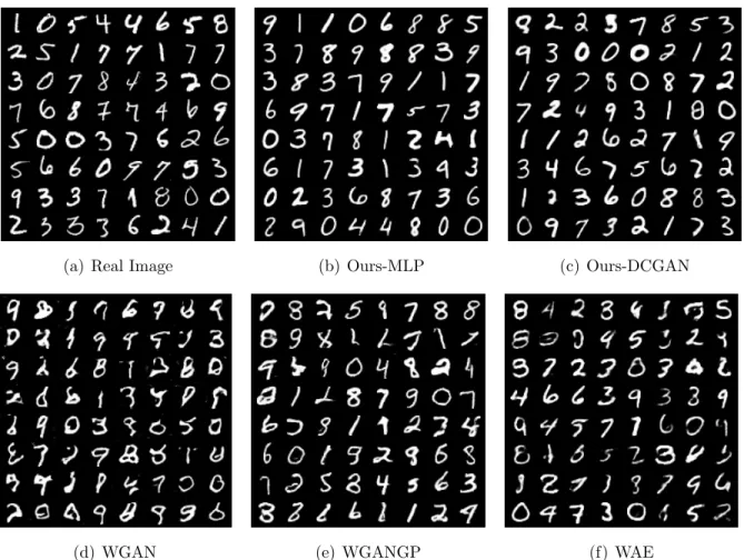
Samples of generated images. Figure 6.4 shows samples generated by different models on the MNIST dataset. The results show that our method with MLP (Figure 6.4(b)) and DCGAN (Figure 6.4(c)) both generate digits with better visual quality than the baselines
with the DCGAN architecture. Figure 6.5 shows the generated samples on Thin-8 by our method, WGANGP, and WAE. The results of WGAN and VAE are omitted as they are similar to both WGANGP and WAE consistently on Thin-8. When MLP is used as the generator architecture, our method again outperforms WGANGP and WAE in terms of the visual quality of the generated samples. When DCGAN is used, the digits generated by our method have slightly worse quality than WGANGP, but better than WAE.
(a) Real Image (b) Ours-MLP (c) Ours-DCGAN
(d) WGAN (e) WGANGP (f) WAE
Figure 6.4: Real and generated samples on the MNIST dataset: (a) real samples; (b) samples generated by our model with MLP as the generator network; (c) samples generated by our model with DCGAN as the generator network; (d) samples generated by WGAN; (e) samples generated by WGANGP; (f) samples generated by WAE. DCGAN is used as the generator architecture in (d)(e)(f).
(a) Ours-MLP (b) WGANGP-MLP (c) WAE-MLP
(d) Ours-DCGAN (e) WGANGP-DCGAN (f) WAE-DCGAN
Figure 6.5: Generated samples on the Thin-8 dataset. (a)(b)(c) are samples generated by different methods using MLP as the generator; and (d)(e)(f) are samples when using DCGAN as the generator.
Importance of the alternating procedure. We use this set of experiments to verify the importance of the alternating procedure that gradually improves the generative network. Figure 6.6 shows: (a) the samples generated by our model; and (b) the samples generated by a weakened version of our model that does not employ the alternating procedure. The non-alternating counterpart derives an optimal transport plan in the first run, and then fits towards the derived plan. It can be seen clearly the samples generated with such a non-alternating procedure have considerably lower visual quality. This verifies the importance of the alternating training procedure: fitting the generator towards the initial OT plan does not provide good enough gradient direction to produce a high-quality generator.
(a) Alternating. (b) Non-alternating.
Figure 6.6: Generated samples on MNIST with and without the alternating procedure.
6.3 QUANTITATIVE RESULTS
We proceed to measure the quantitative performance of the compared models.
MNIST results. Table 6.1 shows the performance of different models on the MNIST training and testing sets. In the first part when MLP is used to instantiate generators, our model achieves the best performance in terms of all the five metrics. The results on neural network distances (NND-WC and NND-GP) are particularly interesting: even though neural network distances are biased in favor of GAN-based models because the adversarial game explicitly optimizes such distances, our model still outperforms GAN-based models without adversarial training. The second part shows the results when DCGAN is the generator architecture. Under this setting, our method achieves the best results among all the metrics except for neural network distances. Comparing the performance of our method on the training and testing sets, one can observe its consistent performance and similar comparisons against baselines. This phenomenon empirically verifies that our method does not overfit.
Table 6.1: Quantitative results on the MNIST training sets.
Method Arch MNIST Training
NND-WC NND-GP WD IS FID WGAN 0.29 5.82 140.710 7.51 31.28 WGANGP 0.13 2.61 107.61 8.89 8.46 VAE MLP 0.53 4.26 101.06 7.10 52.42 WAE 0.18 3.64 90.91 8.42 11.12 Ours 0.11 2.56 66.68 9.77 3.21 WGAN 0.11 4.69 125.63 7.02 27.64 WGANGP 0.08 0.83 93.61 8.65 4.65 VAE DCGAN 0.48 3.68 106.63 6.96 42.10 WAE 0.18 3.29 90.96 8.35 12.28 Ours 0.10 2.28 70.13 9.54 3.76
Table 6.2: Quantitative results on the MNIST testing sets. Note that the Wasserstein distance on training and testing sets of different sizes are not directly comparable.
Method Arch MNIST Test
NND-WC NND-GP WD FID WGAN 0.29 6.05 142.48 31.91 WGANGP 0.12 3.02 112.22 8.99 VAE MLP 0.52 4.42 110.49 51.88 WAE 0.15 3.80 101.46 11.49 Ours 0.10 2.79 82.87 3.56 WGAN 0.10 4.86 132.97 28.44 WGANGP 0.07 1.66 104.15 5.45 VAE DCGAN 0.46 3.89 115.59 41.95 WAE 0.15 3.53 101.02 12.66 Ours 0.09 2.55 82.79 4.18
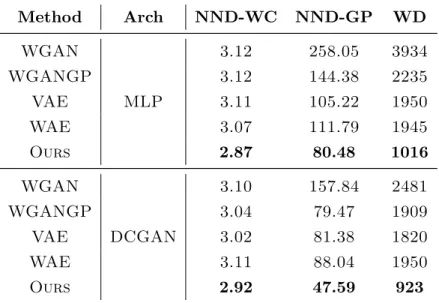
Thin-8 results. There are no meaningful classifiers to compute IS and FID on the Thin-8 dataset. We thus only use NND-WC, NND-GP and WD as the quantitative metrics, and Table 6.3 shows the results. Our method obtains the best results among all the metrics with both the MLP and DCGAN architectures. For NND-WC, all methods expect ours have similar results of around 3.1: we suspect this is due to the weight clipping effect, which is verified by tuning the clipping factor in our exploration. NND-GP and WD have consistent correlations for all the methods. This phenomenon is expected on a small-sized but high-dimensional dataset like Thin-8, because the discriminator neural network has enough capacity to approximate the Lipschitz-1 function class on the samples. The result comparison between NND-WC and NND-GP directly supports the claim [14] that gradient-penalized neural networks (NND-GP) have much higher approximation power than weight-clipped neural networks (NND-WC).
It is interesting to see that WGAN and WGANGP lead to the largest neural net distance and Wasserstein distance, yet their generated samples still have the best visual qualities on Thin-8. This suggests that the success of GAN-based models cannot be solely explained by the restricted approximation power of discriminator [11, 12].
Table 6.3: Quantitative results on the Thin-8 dataset.
Method Arch NND-WC NND-GP WD WGAN 3.12 258.05 3934 WGANGP 3.12 144.38 2235 VAE MLP 3.11 105.22 1950 WAE 3.07 111.79 1945 Ours 2.87 80.48 1016 WGAN 3.10 157.84 2481 WGANGP 3.04 79.47 1909 VAE DCGAN 3.02 81.38 1820 WAE 3.11 88.04 1950 Ours 2.92 47.59 923
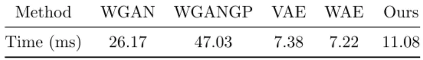
Time cost. Table 6.4 reports the training time of different models on MNIST. For moder-ately sized datasets such as MNIST, our method is faster than WGAN and WGANGP but slower than VAE and WAE. Compared with GAN-based models, our method does not have a discriminator which saves time.
Table 6.4: Training time per iteration of the compared methods on MNIST. Method WGAN WGANGP VAE WAE Ours
CHAPTER 7: EVALUATION OF GANS
In this chapter, we discuss the “side product” of our OTS algorithm: some new metrics to effectively evaluate deep generative models.
7.1 DEFINING NEW METRICS
As discussed in previous sections, now we can exactly computeWasserstein scoreSW(g) :=
Wp(g#µ,ν) of any generator, without any regularization or approximation through neuralˆ
networks, through Algorithm 3.1 and 3.2.
However, using Wasserstein score as the single metric of quality has some drawbacks. When we say a generator does not generate good samples, we are typically referring to one of the following three cases:
1. The generator produces samples that do not correspond to training dataset, for exam-ple images that do not look like digits for MNIST;
2. The generator produces samples that only correspond to a portion of training dataset; 3. The generator simply memorizes the training dataset and can produce nothing beyond
that.
We call the 3 casesunder-approximation,mode collapse andoverfitting, respectively. (The word “mode collapse” has different definitions throughout GAN literature, referring to either Case 2 or Case 3. We define the 2 cases as “mode collapse” and “overfitting” respectively to stress their differences.)
While Wasserstein score is sensitive to all the 3 cases (test dataset is required for over-fitting), as a single score it does not distinguish between the cases. A generator producing blurry images might have the same score as another generator producing sharp images but mode collapse.
This motivates us to define metrics to quantify each case separately. We first define approximation score as follows:
SA(g) := inf
w∈Rn,w0,w>1=nWp(g#µ, w
>
ν) (7.1)
where w 0 means each entry of w is non-negative. Approximation score allows the generator to “choose” a weighted subset of data to achieve the lowest possible Wasserstein distance, i.e. mode collapse to a subset to get highest approximation quality.
While SA can be calculated in dual form similarly to Algorithm 3.1 and 3.2, there is a
simple and intuitive way to calculate by the following proposition:
Proposition 7.1. For p≥1, for any w∈Rn such that w0 and w>1=n,
Wp(µ, w>ν)≥ Ex∼µ inf y∈Supp(ν)kx−yk p p 1/p (7.2) Proof. Letπ be the optimal transport plan between µand w>ν, then
Wpp(µ, w>ν) =E(x,y)∼π(x,y)kx−ykpp ≥E(x,y)∼π(x,y) inf
y∈Supp(ν)kx−yk p p =Ex∼µ inf y∈Supp(ν)kx−yk p p
which concludes the proof.
Lettingwbe the empirical distribution ofLpnearest neighbors, then the following corollary
is directly obtained: Corollary 7.1. SA(g) = Ex∼µ inf y∈Supp(ν)kg(x)−yk p p 1/p . (7.3)
With this corollary, approximation score can be equivalently defined as the expected dis-tance between generated samples and their nearest neighbors.
Building the relationship between Wasserstein distance and nearest neighbors, while being intuitive, is useful since it gives a natural definition of our mode collapse score:
SM(g) :=SW(g)−SA(g) = Wp(g#µ, ν)− inf
w0,w>1=nWp(g#µ, ν) (7.4) WhileSW,SAand SM combined give a comprehensive characterization of how generative
models learn from training dataset, they do not evaluate generators with held-out data. Suppose the underlying distribution of data is ν, and νtrain and νtest are training and test datasets drawn from ν, respectively. A na¨ıve sampling generator which outputs uniform distribution of νtrain will get 0 as all the 3 scores. However, the generator might overfit training dataset and produces samples very different to νtest. This motivates us to define overfitting score as
SO(g) :=Wp(g#µ, νtest)−Wp(g#µ, νtrain) (7.5) By this definition, a generator which generates the underlying distribution ν would have an overfitting score of 0.
7.2 EVALUATION RESULTS
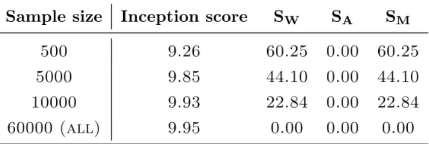
As an example showing how our proposed metrics are useful, Table 7.1 shows inception score and Wasserstein score (p= 1) for a na¨ıve sampling generator which uniformly generates from a subsample of MNIST training dataset. With a fairly large sample size like 10000, nearly perfect inception score can be achieved, neglecting the fact that the generator mode collapses to less than 1/5 of the dataset, which is captured by our proposed metrics.
Table 7.1: Comparing inception score and Wasserstein score for na¨ıve sampling generators.
Sample size Inception score SW SA SM
500 9.26 60.25 0.00 60.25
5000 9.85 44.10 0.00 44.10
10000 9.93 22.84 0.00 22.84
60000 (all) 9.95 0.00 0.00 0.00
We evaluate GAN [4], LSGAN [13], WGAN [5] and WGAN-GP [14] with two types of neural network architecture: MLP and DCGAN [50].
Table 7.2 summarizes our evaluation metrics withp= 1. WGAN-GP works best for MLP architecture while standard GAN works best for DCGAN. It is not surprising that DCGAN has much better mode collapse results than MLP, which stronger generator and discrimina-tor; however, MLP is better at overfitting, possibly because of lower model complexity.
Table 7.2: Evaluation Metrics for the evaluated algorithms.
Algorithm Architecture SW SA SM SW(test) SO MNIST GAN MLP 222.81 101.15 121.67 221.21 -1.60 LSGAN MLP 133.99 92.89 41.10 150.69 16.70 WGAN MLP 73.76 51.07 22.69 74.07 0.31 WGAN-GP MLP 57.36 44.26 13.10 59.24 1.88 GAN DCGAN 42.56 40.07 2.49 48.52 5.96 LSGAN DCGAN 43.42 40.72 2.70 49.04 5.62 WGAN DCGAN 47.59 43.85 3.74 52.22 4.63 WGAN-GP DGGAN 51.34 46.72 4.62 55.09 3.75 CelebA GAN MLP 4186.28 1684.97 2501.31 4254.73 68.45 LSGAN MLP 2227.07 2033.41 193.65 2368.90 141.83 WGAN MLP 2333.05 1306.21 1026.84 2364.11 31.06 WGAN-GP MLP 1850.62 1676.83 173.79 2032.87 182.25 GAN DCGAN 1864.58 1737.57 127.01 2054.75 190.17 LSGAN DCGAN 1869.92 1751.13 118.79 2065.69 195.77 WGAN DCGAN 1986.93 1877.75 109.19 2181.55 194.62 WGAN-GP DCGAN 1889.58 1756.00 131.59 2074.06 184.48
Figure 7.1 qualitatively evaluates how well discriminator loss of WGAN and WGAN-GP can be used to monitor the training process. For all combination except WGAN-GP+DCGAN where training is unstable, decreasing discriminator loss coincides nicely with decreasing Wasserstein score. For WGAN-GP+DCGAN, unstable discriminator losses also coincide with unstable Wasserstein scores. This confirms the practice of using discriminator loss as a training indicator.
10 15 20 25 30 35 40 45 50 Training epoch 58 60 62 64 66 68 70 72 74 Wasserstein Score Wasserstein Score Discriminator Loss 0.00 0.25 0.50 0.75 1.00 1.25 1.50 1.75 Discriminator Loss (a) WGAN+MLP 10 15 20 25 30 35 40 45 50 Training epoch 48 50 52 54 56 58 Wasserstein Score Wasserstein Score Discriminator Loss 0.005 0.006 0.007 0.008 0.009 0.010 0.011 Discriminator Loss (b) WGAN+DCGAN 10 15 20 25 30 35 40 45 50 Training epoch 46 48 50 52 54 56 Wasserstein Score Wasserstein Score Discriminator Loss 0.5 0.6 0.7 0.8 0.9 1.0 Discriminator Loss (c) WGAN-GP+MLP 10 15 20 25 30 35 40 45 50 Training epoch 50 60 70 80 90 Wasserstein Score Wasserstein Score Discriminator Loss 8 10 12 14 16 Discriminator Loss (d) WGAN-GP+DCGAN
CHAPTER 8: DISCUSSION ON LIMITATIONS
We have also run our method on the CelebA and CIFAR10 datasets [52, 53]. On CelebA, our method generates clear faces with good visual quality and with meaningful latent space interpolation, as shown in Figure 8.1(a) and Figure 8.1(b). However, we observe that the good visual quality partly comes from the average face effect: the expressions and back-grounds of generated images lack diversity compared with GAN-based methods.
Figure 8.2 shows the results of our method on CIFAR10. As shown, our method generates identifiable objects, but they are more blurry than GAN-based models. VAE generates objects that are also blurry but less identifiable. We compute the Wasserstein-1 distance of the compared methods on CIFAR10: our method (655), WGAN-GP (849) and VAE (745). Our method achieves the lowest Wasserstein distance but does not have better visual quality than GAN-based models on CIFAR10.
Analyzing these results, we conjecture that minimizing Wasserstein distances on pixel-wise metrics such as`1 and `2 leads to a mode-collapse-free regularization effect. For models that minimize the Wasserstein distance, the primary task inherently tends to cover all the modes disregarding the sharpness of the generated samples. This is because not covering all the modes will result in huge transport cost. In GANs, the primary task is to generate sharp images which can fool the discriminator, and some modes can be dropped towards this goal. Consequently, the objective of our model naturally prevents it from mode collapse, but at the cost of generating more blurry samples. We propose two potential remedies to the blurriness issue: one is to use a perceptual loss; and the other is to incorporate adversarial metric into the framework.
We have tried to apply Lap2 loss similar to [54] (where Lap1 is used): Lap2(x, x0) :=X
j
2−2j|L(j)(x)−L(j)(x0)|2 (8.1) where L(j)(x) is the j-th level of the Laplacian pyramid representation [55] of x.
Figure 8.3 shows the generated images with Lap2loss with a three-layer Laplacian pyramid. The results are slightly better than pixel-wise losses. We will continue exploring this direction in the future.
(a) Generated samples
(b) Latent space walk
(a) Our method
(b) VAE
CHAPTER 9: CONCLUSION
In this thesis, we have proposed a simple alternating procedure to generative modeling by explicitly optimizing the Wasserstein distance between the generated distribution and real data. We show theoretically and empirically that our method does optimize Wasserstein distance to the training dataset, and generalizes to the underlying distribution. We also discuss the evaluation of GANs by our method, and possible directions to accelerate its computation.
There are many interesting future directions in this area. First, entropy-regularized op-timal transport can be used and compared with non-regularized OT. Second, better loss functions including adversarial and perceptual losses should be further studied. Third, the subsampling process might be further improved by some results in the area of nearest neigh-bor search. Finally, a theoretical analysis of how gradual fitting contributes to smoother manifolds and better generalization.
REFERENCES
[1] A. Brock, J. Donahue, and K. Simonyan, “Large scale gan training for high fidelity natural image synthesis,” in ICLR, 2018.
[2] J.-Y. Zhu, T. Park, P. Isola, and A. A. Efros, “Unpaired image-to-image translation using cycle-consistent adversarial networks,” in Proceedings of the IEEE international conference on computer vision, 2017, pp. 2223–2232.
[3] H. Zhu, Q. Liu, N. J. Yuan, C. Qin, J. Li, K. Zhang, G. Zhou, F. Wei, Y. Xu, and E. Chen, “Xiaoice band: A melody and arrangement generation framework for pop mu-sic,” in Proceedings of the 24th ACM SIGKDD International Conference on Knowledge Discovery & Data Mining. ACM, 2018, pp. 2837–2846.
[4] I. J. Goodfellow, J. Pouget-Abadie, M. Mirza, B. Xu, D. Warde-Farley, S. Ozair, A. C. Courville, and Y. Bengio, “Generative adversarial nets,” in NIPS, 2014.
[5] M. Arjovsky, S. Chintala, and L. Bottou, “Wasserstein generative adversarial networks,” in ICML, 2017.
[6] M. G. Bellemare, I. Danihelka, W. Dabney, S. Mohamed, B. Lakshminarayanan, S. Hoyer, and R. Munos, “The cramer distance as a solution to biased wasserstein gradients,” 2017, arXiv:1705.10743 [cs.LG].
[7] A. Genevay, G. Peyr, and M. Cuturi, “Learning generative models with sinkhorn diver-gences,” in AISTATS, 2018.
[8] T. Salimans, H. Zhang, A. Radford, and D. Metaxas, “Improving GANs using optimal transport,” in ICLR, 2018.
[9] H. Liu, G. Xianfeng, and D. Samaras, “A two-step computation of the exact gan wasser-stein distance,” in ICML, 2018.
[10] B. Sriperumbudur, K. Fukumizu, A. Gretton, B. Sch¨olkopf, and G. Lanckriet, “On the empirical estimation of integral probability metrics,” Electronic Journal of Statistics, vol. 6, pp. 1550–1599, 2012.
[11] S. Arora, R. Ge, Y. Liang, T. Ma, and Y. Zhang, “Generalization and equilibrium in generative adversarial nets (GANs),” in ICML, 2017.
[12] G. Huang, G. Gidel, H. Berard, A. Touati, and S. Lacoste-Julien, “Adversarial di-vergences are good task losses for generative modeling,” 2017, arXiv:1708.02511 [cs.LG].
[13] X. Mao, Q. Li, H. Xie, R. Y. Lau, Z. Wang, and S. P. Smolley, “Least squares generative adversarial networks,” arXiv:1611.04076 [cs.CV].
[14] I. Gulrajani, F. Ahmed, M. Arjovsky, V. Dumoulin, and A. C. Courville, “Improved training of wasserstein GANs,” in NIPS, 2017.
[15] C. Villani,Topics in Optimal Transportation. American Mathematical Society, 2003. [16] C. Villani,Optimal Transport: Old and New. Springer, 2009.
[17] G. Peyr´e and M. Cuturi, “Computational optimal transport,” 2018,arXiv:1803.00567 [stat.ML].
[18] N. Lei, K. Su, L. Cui, S.-T. Yau, and X. D. Gu, “A geometric view of optimal trans-portation and generative model,” Computer Aided Geometric Design, vol. 68, pp. 1–21, 2019.
[19] A. Genevay, M. Cuturi, G. Peyr´e, and F. R. Bach, “Stochastic optimization for large-scale optimal transport,” in NIPS, 2016.
[20] V. Seguy, B. B. Damodaran, R. Flamary, N. Courty, A. Rolet, and M. Blondel, “Large-scale optimal transport and mapping estimation,” in ICLR, 2018.
[21] M. Cuturi, “Sinkhorn distances: Lightspeed computation of optimal transport,” in NIPS, 2013.
[22] R. Sinkhorn, “A relationship between arbitrary positive matrices and doubly stochastic matrices,” Ann. Math. Statist., vol. 35, no. 2, pp. 876–879, 06 1964.
[23] D. P. Kingma and M. Welling, “Auto-encoding variational bayes,” in ICLR, 2014. [24] C. Doersch, “Tutorial on variational autoencoders,” arXiv preprint arXiv:1606.05908,
2016.
[25] M. Arjovsky and L. Bottou, “Towards principled methods for training generative ad-versarial networks,” in ICLR, 2017.
[26] O. Bousquet, S. Gelly, I. Tolstikhin, C.-J. Simon-Gabriel, and B. Schoelkopf, “From optimal transport to generative modeling: the VEGAN cookbook,” 2017,
arXiv:1705.07642 [stat.ML].
[27] I. Tolstikhin, O. Bousquet, S. Gelly, and B. Schoelkopf, “Wasserstein auto-encoders,” 2017, arXiv:1711.01558.
[28] A. Genevay, G. Peyr´e, and M. Cuturi, “GAN and VAE from an optimal transport point of view,” 2017, arXiv:1706.01807 [stat.ML].
[29] Y. Xie, X. Wang, R. Wang, and H. Zha, “A fast proximal point method for wasserstein distance,” 2018, arXiv:1802.04307 [stat.ML].
[30] L. Theis, A. van den Oord, and M. Bethge, “A note on the evaluation of generative models,” in ICLR, 2016.
[31] I. Goodfellow, Y. Bengio, and A. Courville, Deep Learning. MIT Press, 2016, http://www.deeplearningbook.org.
[32] A. Borji, “Pros and cons of GAN evaluation measures,” 2018, arXiv:1802.03446 [cs.CV].
[33] T. Salimans, I. J. Goodfellow, W. Zaremba, V. Cheung, A. Radford, and X. Chen, “Improved techniques for training GANs,” 2016, arxiv:1606.03498 [cs.LG].
[34] T. Che, Y. Li, A. P. Jacob, Y. Bengio, and W. Li, “Mode regularized generative adver-sarial networks,” in ICLR, 2017.
[35] Z. Zhou, H. Cai, S. Rong, Y. Song, K. Ren, J. Wang, W. Zhang, and Y. Yong, “Acti-vation maximization generative adversarial nets,” in ICLR, 2018.
[36] H. Heusel, H. Ramsauer, T. Unterthiner, and B. Nessler, “GANs trained by a two time-scale update rule converge to a local nash equilibrium,” in NIPS, 2017.
[37] A. Gretton, K. M. Borgwardt, M. J. Rasch, B. Sch¨olkopf, and A. Smola, “A kernel two-sample test,” Journal of Machine Learning Research, vol. 13, pp. 723–773, 2012. [38] D. J. Sutherland, H.-Y. Tung, H. Strathmann, S. De, A. Ramdas, A. Smola, and
A. Gretton, “Generative models and model criticism via optimized maximum mean discrepancy,” in ICLR, 2018.
[39] M. Lucic, K. Kurach, M. Michalski, S. Gelly, and O. Bousquet, “Are GANs created equal? a large-scale study,” arXiv:1711.10337 [stat.ML].
[40] I. Danihelka, B. Lakshminarayanan, B. Uria, D. Wierstra, and P. Dayan, “Compari-son of maximum likelihood and gan-based training of real NVPs,” arXiv:1705.05263 [cs.LG].
[41] D. J. Im, H. Ma, G. Taylor, and K. Branson, “Quantitatively evaluating GANs with divergences proposed for training,” in ICLR, 2018.
[42] S. Arora and Y. Zhang, “Do GANs actually learn the distribution? an empirical study,” 2017, arXiv:1706.08224 [cs.LG].
[43] A. Srivastava, L. Valkov, C. Russell, and M. U. Gutmann, “Veegan: Reducing mode collapse in GANs using implicit variational learning,” in NIPS, 2017.
[44] Y. Bai, T. Ma, and A. Risteski, “Approximability of discriminators implies diversity in GANs,” in ICLR, 2019.
[45] K. Hornik, M. Stinchcombe, and H. White, “Multilayer feedforward networks are uni-versal approximators,” Neural Networks, vol. 2, no. 5, pp. 359–366, july 1989.
[46] G. Cybenko, “Approximation by superpositions of a sigmoidal function,” Mathematics of Control, Signals and Systems, vol. 2, no. 4, pp. 303–314, 1989.
[47] D. Yarotsky, “Error bounds for approximations with deep relu networks,” 2016,
arXiv:1610.01145 [cs.LG].
[48] M. Anthony and P. L. Bartlett, Neural Network Learning: Theoretical Foundations. Cambridge University Press, 1999.
[49] Y. Lecun, L. Bottou, Y. Bengio, and P. Haffner, “Gradient-based learning applied to document recognition,” in Proceedings of the IEEE, 1998, pp. 2278–2324.
[50] A. Radford, L. Metz, and S. Chintala, “Unsupervised representation learning with deep convolutional generative adversarial networks,” 2015, arXiv:1511.06434 [cs.LG]. [51] S. Ioffe and C. Szegedy, “Batch normalization: Accelerating deep network training by
reducing internal covariate shift,” 2015, http://arxiv.org/abs/1502.03167.
[52] Z. Liu, P. Luo, X. Wang, and X. Tang, “Deep learning face attributes in the wild,” in ICCV, 2015.
[53] A. Krizhevsky, “Learning multiple layers of features from tiny images,” Citeseer, Tech. Rep., 2009.
[54] P. Bojanowski, A. Joulin, D. Lopez-Pas, and A. Szlam, “Optimizing the latent space of generative networks,” in ICML, 2018.
[55] H. Ling and K. Okada, “Diffusion distance for histogram comparison,” in 2006 IEEE Computer Society Conference on Computer Vision and Pattern Recognition (CVPR’06), vol. 1. IEEE, 2006, pp. 246–253.