Universidade de São Paulo
2015-02
An extensive evaluation of decision tree-based
hierarchical multilabel classification methods
and performance measures
Computational Intelligence, Malden, v. 31, n. 1, p. 1-46, Feb. 2015
http://www.producao.usp.br/handle/BDPI/50039
Downloaded from: Biblioteca Digital da Produção Intelectual - BDPI, Universidade de São Paulo
Biblioteca Digital da Produção Intelectual - BDPI
AN EXTENSIVE EVALUATION OF DECISION TREE–BASED
HIERARCHICAL MULTILABEL CLASSIFICATION METHODS AND
PERFORMANCE MEASURES
RICARDOCERRI,1GISELEL. PAPPA,2ANDRÉCARLOSP. L. F. CARVALHO,1
ANDALEXA. FREITAS3
1Departamento de Ciências de Computação, Universidade de São Paulo, Campus de São Carlos,
São Carlos, SP, Brazil
2Departamento de Ciências da Computação, Universidade Federal de Minas Gerais, Belo Horizonte,
MG, Brazil
3School of Computing, University of Kent, Canterbury, Kent, UK
Hierarchical multilabel classification is a complex classification problem where an instance can be assigned to more than one class simultaneously, and these classes are hierarchically organized with superclasses and subclasses, that is, an instance can be classified as belonging to more than one path in the hierarchical structure. This article experimentally analyses the behavior of different decision tree–based hierarchical multilabel classification methods based on the local and global classification approaches. The approaches are compared using distinct hierarchy-based and distance-based evaluation measures, when they are applied to a variation of real multilabel and hierarchical datasets’ characteristics. Also, the different evaluation measures investigated are compared according to their degrees of consistency, discriminancy, and indifferency. As a result of the experimental analysis, we recommend the use of the global classification approach and suggest the use of the Hierarchical Precision and Hierarchical Recall evaluation measures.
Received 31 March 2011; Revised 6 June 2012; Accepted 28 December 2012
Key words: hierarchical, multilabel, classification, performance measures, global and local approaches.
1. INTRODUCTION
In most of the classification problems described in the literature, a classifier assigns a
single class to a given instancexi, and the classes form a nonhierarchical, flat structure, with
no consideration of superclasses or subclasses. However, in many real-world classification problems, one or more classes can be divided into subclasses or grouped into superclasses, and instances can belong to more than one class simultaneously at a same hierarchical level. In this case, the classes follow a hierarchical structure, usually a tree or a directed acyclic graph (DAG). These problems are known in the literature of machine learning as hierarchi-cal multilabel classification (HMC) problems. They are more complex than conventional classification problems, which are flat and single-label, because new instances can be classi-fied into the classes associated with two or more paths in the class hierarchy. These problems are very common, for example, in the classification of genes and identification of protein functions (Blockeel et al. 2002; Clare and King 2003; Struyf, Blockeel, and Clare 2005; Kiritchenko, Matwin, and Famili 2005; Barutcuoglu, Schapire, and Troyanskaya 2006; Vens et al. 2008; Alves, Delgado, and Freitas 2008; Obozinski et al. 2008; Valentini 2009, 2011; Alves, Delgado, and Freitas 2010; Schietgat et al. 2010; Otero, Freitas, and Johnson 2010; Cerri, Carvalho, and Freitas 2011; Cerri and Carvalho 2011; Pugelj and Džeroski 2011; Bi and Kwok 2011), and text classification (Sun and Lim 2001; Kiritchenko, Matwin, and Famili 2004; Rousu et al. 2006; Cesa-Bianchi, Gentile, and Zaniboni 2006; Mayne and
Address correspondence to Ricardo Cerri, Departamento de Ciências de Computação, Universidade de São Paulo, Campus de São Carlos, Av. Trabalhador São-carlense, 400, Centro, 13560-970, São Carlos, SP, Brazil; e-mail: [email protected]
Perry 2009). HMC problems can be defined as complex classification problems, which encompass the characteristics of both hierarchical single-label problems and nonhierarchical multilabel problems.
In hierarchical single-label classification problems, each instance is assigned to a sin-gle path of the hierarchical structure. The process of classification of new instances may be a mandatory leaf node classification, when a new instance must be assigned to a leaf node, or a nonmandatory leaf node classification, when the most specific class assigned to a new instance can be an internal (nonleaf) node of the class hierarchy (Freitas and Carvalho 2007). Two approaches have been adopted in the literature to deal with the class hierarchy in hierarchical problems: top–down or local and one-shot or global.
The local approach uses local information to consider the hierarchy of classes. During the training phase, the hierarchy of classes is processed level by level, producing one or more classifiers for each level of the hierarchy. This process produces a tree of classifiers. The root classifier is induced with all training instances. At each other level, a classifier is induced using just local instances associated with classes at that level. In the test phase, when an instance is assigned to a class that is not a leaf node, it is further classified into one subclass of this class. A deficiency of this approach is the propagation of classification errors in a class node to its descendant nodes in the class hierarchy. However, it allows the use of any traditional classification algorithm, because each local classification algorithm is a conventional, flat classification algorithm.
The global approach induces a unique classification model considering the class hier-archy as a whole, avoiding the error propagation problem of the local approach. After the model induction, the classification of a new instance occurs in just one step. Hence, tradi-tional classification algorithms cannot be used, unless adaptations are made to consider the hierarchy of classes.
In nonhierarchical multilabel problems, each instance can be assigned to one or more classes simultaneously. Similar to hierarchical single-label problems, where the local and global approaches can be used to solve the classification task, two main approaches can be used to solve nonhierarchical multilabel problems, named algorithm dependent and algorithm independent (Carvalho and Freitas 2009). The algorithm independent approach transforms the original multilabel problem into a set of single-label problems and, as in the local approach for hierarchical problems, any traditional classification algorithm can be used. In the algorithm dependent approach, as the name suggests, new algorithms are devel-oped specifically for multilabel problems, or traditional algorithms are modified to cope with these problems. The global approach used in hierarchical problems can be seen as an algorithm dependent approach, as new or modified algorithms are used.
In HMC problems, the characteristics of the hierarchical and multilabel problems are combined, and an instance can be assigned to two or more subtrees of the class hierarchy. As stated by Vens et al. (2008), the HMC problem can be formally described as follows: Given:
a space of instancesX;
a class hierarchy.C;h/, whereC is a set of classes andh is a partial order
repre-senting the superclass relationship (for allc1; c2 2 C W c1 h c2if and only ifc1is a
superclass ofc2);
a setT of tuples (xi; Ci) withxi 2 XandCi C, such thatc 2Ci ) 8c0 h c Wc0 2
Ci;
Find:
a functionf W X!2C, where2C is the powerset ofC, such thatc 2f .x/ ) 8c0 h
c Wc0 2f .x/andf optimizesq.
The quality criterion q can be the mean accuracy of the predicted classes or the
dis-tances between the predicted and true classes in the class hierarchy. It can also consider that misclassifications in levels closer to the root node are worse than misclassifications in deeper levels. Besides, the complexity of the classifiers and the induction time can be taken into account as quality criteria.
Although the given HMC definition says that an instance belongs to and has to be classi-fied into proper hierarchical paths, there are some works that allow inconsistent predictions. Examples are the works of Cesa-Bianchi et al. (2006), Kiritchenko et al. (2006), Obozinski et al. (2008), Valentini (2011), and Cerri and Carvalho (2011), where predictions inconsis-tent with the hierarchy are made, and then an additional step of making the class assignments consistent with the hierarchy is required.
An example of HMC problem is illustrated in Figure 1, where the class hierarchy is represented by a tree. In this example, a newspaper report can address subjects related to computer sciences and soccer and, therefore, be classified into both sciences/computing and sports/collective/soccer classes. The class prediction for a new instance generates a subtree. In the figure, the nodes with a rectangle and the nodes with an ellipse represent two pre-dicted paths in the tree for a new instance, sciences/computing and sports/collective/soccer, respectively.
There are several works proposing HMC methods and using HMC or flat performance measures for specific datasets (Sun and Lim 2001; Vens et al. 2008; Alves et al. 2010; Otero et al. 2010; Cerri et al. 2011; Cerri and Carvalho 2011; Pugelj and Džeroski 2011; Bi and Kwok 2011). The work of Ceci and Malerba (2007) evaluates hierarchical classi-fiers using flat (nonhierarchical) evaluation measures. In Sokolova and Lapalme (2009), a series of flat, multilabel, and hierarchical evaluation measures were analyzed according to the type of changes to a confusion matrix that do not change a measure, but the analyses were only theoretical. In Brucker, Benites, and Sapozhnikova (2011), the authors performed experiments with a series of flat multilabel classifiers. Hierarchies were then extracted from the flat results obtained, and then hierarchical and flat classification measures were used in
FIGURE1. Hierarchical multilabel classification problem structured as a tree: (a) class hierarchy and (b)
the evaluation. In Silla and Freitas (2010), HMC evaluation measures were analyzed, but no experiments were performed comparing the measures.
Although these works compare different methods and measures, we did not find guidelines associating the characteristics of hierarchical and multilabel datasets to the per-formance of different methods evaluated by distinct HMC perper-formance measures. This paper experimentally compares different HMC methods and different HMC predictive per-formance measures specific for HMC problems. More precisely, the main contributions of this work are the following:
The evaluation and comparison of hierarchy-based and distance–based predictive
perfor-mance measures, which are specific for HMC problems, when used in a collection of 12 real datasets with different hierarchical and multilabel characteristics.
The analysis of the predictive performance of four different decision tree–based HMC
methods, two of them based on the local approach and two based on the global approach, in these 12 datasets.
In our experimental analysis, we vary four different characteristics of HMC problems, as follows: (i) the percentage of multilabel instances, (ii) the number of classes assigned to an instance, (iii) the unbalance of the class hierarchy, and (iv) the maximum number of child nodes per internal node. The experiments were designed to investigate the effect of different values of those problem characteristics (corresponding to different datasets) in the results of four decision tree–based HMC methods (two based on the local approach and two based on the global approach), as evaluated by ten different performance evaluation measures. More precisely, for each of the aforementioned four problem (dataset) characteristics being varied, we address the following research questions:
Q1:Does a specific evaluation measure favor a specific classification approach (global
or local) when used to compare global and local-based methods?
Q2:Which classification approach (global or local) is better overall, considering the four
aforementioned classification scenarios?
Q3:Are global/local methods better in predicting more specific/general classes?
Q4:How different hierarchical and multilabel characteristics influence different
evalua-tion measures?
Q5: Which evaluation measure is more suitable to use in the classification scenarios
investigated?
For the experiments performed in this work, we have chosen methods that induce deci-sion trees, because there are works that have already shown that decideci-sion trees are a good alternative for HMC classification (Clare and King 2003; Vens et al. 2008; Alves et al. 2010; Otero et al. 2010) and also because the classifiers produced are interpretable.
The rest of this article is organized as follows: Section 2 reviews the hierarchical clas-sification performance measures used in this work. Section 3 presents the HMC methods used in the experiments performed in this work. The experiments carried out are described in Section 4, together with an analysis of the results obtained. Finally, Section 5 presents the main conclusions regarding the experimental results and suggestions for future work.
2. REVIEW OF EVALUATION MEASURES
Classification accuracy measures for conventional (flat) classification problems are usually inadequate for hierarchical multilabel problems. Apart from not considering the
problem’s hierarchical class structure, and the fact that an instance can simultaneously belong to more than one class, conventional classification accuracy measures ignore that the difficulty of classification usually increases with the depth of the classes to be pre-dicted. In hierarchical classification, more specific classes are often harder to predict than generic ones, and conventional measures assume misclassification costs to be indepen-dent of the positions of classes in the hierarchy. Furthermore, in multilabel classification, these measures do not consider that an instance can be assigned to just a subset of its true classes.
As alternatives to conventional evaluation measures for classification problems, spe-cific measures for hierarchical, multilabel, and hierarchical multilabel classifiers have been proposed. Here, we are interested in two broad groups of hierarchical multilabel evaluation measures, namely (i) hierarchy-based evaluation measures and (ii) distance-based evaluation measures. Whereas hierarchy-based measures are based only on the hierarchical class struc-ture (only subclasses and superclasses), distance-based measures also consider the distance between the predicted and true classes in the hierarchy structure.
Although many works in the literature evaluate the performance of hierarchical multil-abel classifiers, there is no consensus on which measure is more appropriate to which type of dataset or method. This section reviews the evaluation measures used in this work and discusses their pros and cons, to later contrast them in experiments involving datasets with different characteristics and different HMC methods.
2.1. Hierarchy-Based Evaluation Measures
Hierarchy-based evaluation measures consider both the ancestors and the descendants of the predicted classes in the hierarchy when evaluating a classifier. In Section 2.1.1, we discuss two variations of hierarchical precision and recall, and in Section 2.1.2, we present the hierarchical loss function, which is based on the traditional 0/1-loss measure.
2.1.1. Hierarchical Precision and Recall. In Kiritchenko et al. (2004), two evalua-tion measures based on the convenevalua-tional precision and recall measures were proposed to take into account hierarchical relationships between classes. These two measures, named hierarchical precision and hierarchical recall, were formally defined in the work of Kiritchenko et al. (2005). These evaluation measures were later used in Eisner et al. (2005) and Kiritchenko et al. (2006).
The hierarchical precision and recall measures consider that an instance belongs not only to its predicted classes but also to all its ancestor classes in the hierarchical structure.
Hence, given an instancexi; Ci0, wherexi belongs to the spaceXof instances,Ci0 is the
set of predicted classes forxi, andCi is the set of true classes ofxi, the setsCi andCi0can
be extended to contain their correspondingancestor classesasCbi DSck2CiAncestors.ck/
and Cb0i D Scl2Ci0Ancestors.cl/, where Ancestors.ck/ denotes the set of ancestors of
classck.
Equations (1) and (2) present the hierarchical precision and recall (hP andhR)
mea-sures. These measures count the number of classes correctly predicted, together with the number of ancestor classes correctly predicted (Kiritchenko et al. 2005). Figure 2 presents an example of how to calculate these measures. In the figure, each set of two hierar-chical structures, one above and one below, represents the true and predicted classes for an instance. In Figure 2(a), solid circles represent the true classes of an instance,
FIGURE2. Graphical example of the use of the hierarchical precision and recall measures: (a) true classes and (b) predicted classes. Adapted from the work of Kiritchenko et al. (2004).
and in Figure 2(b), bold circles represent the predicted classes of the corresponding aforementioned instance, with an arrow showing the deepest predicted class.
hP D P i ˇ ˇ ˇbCi\bC0i ˇ ˇ ˇ P i ˇ ˇ ˇbC0iˇˇˇ (1) hRD P i ˇ ˇ ˇbCi\Cb0i ˇ ˇ ˇ P i ˇ ˇ ˇbCi ˇ ˇ ˇ (2)
As can be seen, all nodes in the path from the root node to the predicted class node for an instance are bold, indicating that the ancestor classes of the predicted classes are also assigned to the instance. The edges from the root node to the node that represents the
deepest predicted class of an instance are also shown in bold. ThehP andhRvalues for the
three different predictions are also illustrated in the figure.
Either hierarchical precision or hierarchical recall used alone is not adequate for the evaluation of hierarchical classifiers (Sebastiani 2002). Both measures have to be considered
together or combined in a single F-measure. Thus, thehP andhRmeasures are combined
on a hierarchical extension of the F-measure, named Hierarchical-Fˇ, presented in equation
(3). In equation (3),ˇ represents the importance assigned to the values ofhP andhR. As
the value ofˇincreases, the weight assigned to the value ofhRalso increases. On the other
hand, when the value ofˇdecreases, the weight assigned tohP increases.
HierarchicalFˇ D
.ˇ2C1/hP hR
ˇ2hP ChR (3)
In the same direction as Kiritchenko et al. (2005), Ipeirotis, Gravano, and Sahami (2001) also measured the hierarchical precision and recall for an instance through the intersection of the predicted and true classes. However, unlike the definitions of hierarchical precision and recall previously described, Ipeirotis et al. (2001) expanded the set of true and predicted
classes by including all their subclasses instead of their superclasses. Thus, given the set
of predicted Ci0and true .Ci/ classes, they are extended to contain their corresponding
descendant classesas:Cb0i DSck2C0
iDescendants.ck/andCbi D
S
cl2CiDescendants.cl/,
whereDescendants.ck/denotes the set of descendants of the classck. This new definition of
b
C0i andCbican be directly used in the formulas presented in equations (1) and (2). Although
the authors claimed that this measure captures the nuances of hierarchical classification, we do not think it is totally correct for the HMC task, because expanding a set of classes to contain their corresponding subclasses can result in a wrong classification. As an example, if a document is classified in the class “sports,” it is not necessarily classified in both subclasses “basketball” and “soccer.”
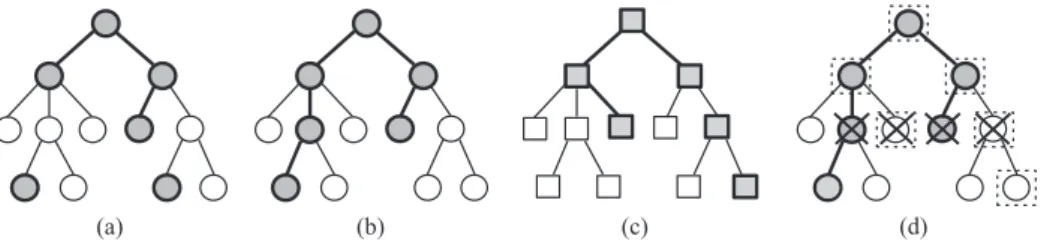
2.1.2. Hierarchical Loss Function. The hierarchical loss function (H-Loss), proposed in Cesa-Bianchi et al. (2006), is based on the concept that, when a misclassification occurs in a class of the hierarchy, no additional penalizations should be given to misclassifications
in the subtree of this class. That is, if a misclassification occurs in classcj0, additional errors
in the subtree rooted atcj0 are not important. As an example, if a classifier erroneously
clas-sifies a document as belonging to the class “sports,” this classifier should not be penalized again by erroneously classifying it in the subclass “soccer.”
Consider that the set of true classes assigned to a given instancexi is any subset of the
set C formed by all classes, including the empty set. This subset is represented by a
vec-tor .c1; : : : ; cjCj/, where a class cj belongs to the subset of classes of instance xi if and
only ifcj D 1. Before defining the H-Loss function, two measures regarding the
discrep-ancy between a multilabel prediction for xi
C0 Dc10; : : : ; cj0Cj, and the true set of
classes of xi .C D .c1; : : : ; cjCj//, for each instance, need to be introduced. The first is
the zero-one loss.l0=1.C; C0//, presented in equation (4). The second is the symmetric
dif-ference loss.l.C; C0//, defined in equation (5). Note that these equations do not consider
the hierarchical structure of the problem, only multiple labels. On the basis of these two
measures, Cesa-Bianchi et al. (2006) proposed the H-Loss function .lH.C; C0//, defined
in equation (6). In the equations, 1¹ºis an indicator function that yields 1 if the provided
equation is true and 0 otherwise.
l0=1.C; C0/D1; if 9j 2 ¹1; : : : ;jCjº Wcj ¤cj0 (4) l.C; C0/D jCj X jD1 1®cj ¤cj0 ¯ (5) lH.C; C0/D jCj X jD1 1®cj ¤cj0 ^Ancestors.cj/DAncestorsc0j ¯ (6)
This measure is based on the fact that, given a hierarchical structureG, this structure
can be considered a forest composed by trees defined on the set of classes of the problem.
A multilabel classification C0 2 ¹0; 1ºjCj respects the structureGif and only if C0 is the
union of one or more paths ofG, where each path starts in a root class and not necessarily
ends up in a leaf class. Hence, all paths ofG, from a root class to a leaf class, are examined.
FIGURE3. Graphical representation of the H-Loss function. Adapted from the work of Cesa-Bianchi et al. (2006).
predictions in the subtrees rooted in the classcj0 are discarded. Given this definition, we can
say thatl0=1lH l.
Figure 3 shows the concepts and use of the H-Loss function. In the four class hierarchies illustrated, round gray nodes represent the classes being predicted for an instance, whereas squared gray nodes represent the true classes of the instance. Note that in Figure 3(a), the
classes predicted do not respect the hierarchical structure of G (parents of predicted leaf
nodes are not predicted), whereas in Figure 3(b), the structure is respected. Figure 3(c) shows the true classes of the instance classified in Figure 3(b), and Figure 3(d) shows the application of the H-Loss function considering the multilabel classifications illustrated in (b) and (c). Only the nodes marked with an “X” are considered when calculating the H-Loss. As can be seen, the values of the zero-one loss and symmetric difference loss functions are 1 and 6, respectively. The H-Loss function returns the value 4. Recall that the lower the value of the function H-Loss, the better the performance of the classifier.
As the hierarchical loss function measure ignores errors in subtrees of classes erro-neously assigned to instances, the error propagation problem present in hierarchical classification is not taken into account. Hence, although some authors work with this measure, it cannot be easily compared with others in the literature.
2.2. Distance-Based Evaluation Measures
This class of measures is based on the assumption that closer classes in the hierarchy tend to be more similar to each other (representing a smaller classification error) than distant classes. Hence, these measures consider the distance between the true and predicted classes during evaluation. Section 2.2.1 reviews the micro/macro distance-based hierarchical pre-cision and micro/macro distance-based hierarchical recall, and Section 2.2.2 discusses the most common ways of calculating distances between hierarchy nodes.
2.2.1. Micro/Macro Distance-Based Hierarchical Precision and Recall. The micro/ macro hierarchical precision and micro/macro hierarchical recall measures, proposed by Sun and Lim (2001), are based on the distance between predicted and true classes. The macro hierarchical precision and recall initially calculate the performance obtained in each class separately and return the average of these values for each measure. The micro hier-archical precision and recall measures, on the other hand, calculate the average of the performance obtained in each instance of a dataset. Hence, whereas the macro measures are considered a per class mean performance measure, the micro measures are considered a per instance mean performance measure (Yang 1999).
For each of these measures, it is necessary to first define, for each class, thecontribution
of the instances erroneously assigned to that class. This contribution is defined according to
an acceptable distance (number of edges (Dis)) between a predicted and a true class, which
that are “slightly” misclassified (with just two edges between the predicted and true class in the class hierarchy) give zero contribution in the calculation of the measures, whereas the instances that are more seriously misclassified (with more than two edges between the predicted and true class) contribute negatively to the values of the measures. Equations (7)
and (8) specify the contribution of an instance xi to a classcj, where xi:agd andxi:lbd
are, respectively, the predicted and true classes of xi. Dis
c; cj0is the distance between
a true class c and a predicted classc0j and can be calculated using any of the approaches
described in Section 2.2.2. Ifxi is a false positive: Conxi; cj0 D X c2xi:lbd 0 @1:0 Disc; cj0 Dis 1 A (7) Ifxi is a false negative: Conxi; cj0 D X c2xi:agd 0 @1:0 Disc; cj0 Dis 1 A (8)
The contribution of an instance xi is then restricted to the values Œ1; 1. This
refinement, denoted byRConxi; cj0
, is defined in equation (9).
RConxi; cj0
Dmin1;max1;Conxi; cj0
(9)
The total contribution of false positives (FP) .FpConj/ and false negatives (FN)
.FnConj/, for all instances, is defined in equations (10) and (11).
FpConj D X xi2FPj RConxi; cj0 (10) FnConj D X xi2F Nj RConxi; cj0 (11)
After the calculation of the contributions of each instance, the values of the hierarchical precision and recall for each class are calculated as defined in equations (12) and (13).
P rjCD D
max.0;jTPjj CFpConj CFnConj/
jTPjj C jFPjj CFnConj
(12)
RejCD D max.0;jTPjj CFpConj CFnConj/ jTPjj C jF Njj CFpConj
(13) Finally, the extended values of hierarchical precision and recall (hierarchical micro
of classes. According to the value ofDis, the values ofFpConj andFnConj can be nega-tive. Therefore, a max function is applied to the numerators of the equations (14) and (15)
to make their values not lower than zero. AsFpConj jFPjj, whenjTPjj C jFPjj C
FnConj 0, the numerator max.0;jTPjj CFpConj CFnConj/ D0. TheP rO CD
value
can be considered zero in this case. The same rule is applied to the calculation ofReO CD
(Sun and Lim 2001).
O
P rCD D
Pm
jD1.max.0;jTPjj CFpConj CFnConj//
Pm jD1.jTPjj C jFPjj CFnConj/ (14) O ReCDD Pm
jD1.max.0;jTPjj CFpConj CFnConj//
Pm
jD1.jTPjj C jF Njj CFpConj/
(15) The hierarchical macro precision and the hierarchical macro recall measures can also
be obtained using equations (16) and (17), wheremrepresents the number of classes.
O P rMCD D Pm jD1P rjCD m (16) O ReMCD D Pm jD1RejCD m (17)
Just like the hP and hR measures, used in the work of Kiritchenko et al. (2005),
the hierarchical micro/macro precision and recall measures can also be combined into the
Hierarchical-Fˇ measure (equation (3)).
2.2.2. Methods for Calculating Distances Between Classes. The micro/macro hierar-chical precision and recall use the distance between two classes in the hierarchy to evaluate the predictions made by a classifier. This section describes a few methods that can be employed to calculate these distances, which are usually defined as a function of two com-ponents: (i) the number of edges between the predicted class and the true class and (ii) the depth of the predicted and true classes in the hierarchy.
The most common method, used in the standard version of measures, is to consider the distance as the number of edges that separate the true and predicted classes. Additionally, weights can be assigned to each edge of the class hierarchy, so that the misclassification between the predicted and true classes is given by the sum of the weights of the edges in the path between the two classes.
There are different ways of calculating the paths between classes depending on the hier-archy structured being considered. If the structure is a tree, there can be only one path between two classes, but if the hierarchy is a DAG, there can be more than one path between two classes, based on the number of superclasses of a class. In the final classification, one
can consider two interpretations of the class hierarchy: if an instance belongs to a classcj,
it belongs to all superclasses ofcj, or it belongs to at least one superclass ofcj. Although
in theory, an evaluation measure could indeed use any of the previous two types of inter-pretation, in practice, only the former (a class belongs to all its superclasses) is used and corresponds to the HMC definition we use in this paper.
Moreover, in the experiments performed, we consider only hierarchies structured as trees, as carried out in the works of Wang et al. (1999) and Dekel et al. (2004). When using
hierarchies structured as trees, Wang et al. (1999) considered the distances between the true and predicted classes in a hierarchical structure in order to rank hierarchical classification rules. They defined the distance between two classes as the shortest path (number of edges) between the classes. Dekel et al. (2004) also used the distances between true and predicted classes in a tree hierarchy to evaluate a final classification. However, in the latter, the authors
defined a distance functioncj; cj0
as the number of edges in the unique path between a
true classcj and a predicted classcj0.
To consider the importance of the classes according to the levels they belong to, there are many ways of choosing weights for edges. One of the most common is to consider that weights of edges at deeper levels should be lower than weights of edges in higher levels. Holden and Freitas (2006), for example, assigned weights that were exponentially decre-mented as the depth of the edges in a tree hierarchy increased. In the work of Vens et al. (2008), the authors proposed a weighting technique that can be applied to DAG and tree
hierarchies. The authors defined the weight of a classcj as the recurrence relationw.cj/D
w0w.par.cj//, with par.cj/ being the parent class of cj, and the weights assigned to
the first level classes equal tow0. The generalization for DAG hierarchies can be obtained
replacing w.par.cj//by an aggregation function (sum;min;max;average) computed over
the weights assigned to the parents of classcj (Vens et al. 2008). Assigning weights to the
edges of the hierarchy, however, presents some problems, especially when the hierarchy is very unbalanced, and its depth varies significantly by different leaf nodes. In this case, a mis-classification involving predicted and true classes near the root node receives a lower penal-ization than a misclassification involving classes at levels more distant from the root node. In this direction, Lord et al. (2003) showed that when two classes are located in different subtrees of the hierarchy, and the route between them has to go through the root node, the fact that one class is in a deeper level than the other does not necessarily means that the class located in the deeper level provides more significant information than the class located in the
higher level. Therefore, considering depth without considering the information associated with the classes may be a problem.
Figure 4 illustrates the problem of assigning weights to edges of a hierarchy. Here, the filled ellipses represent the true classes of an instance and the bold ellipses represent the predicted classes. Consider an instance that belongs to class “11.04.03.01” (True), and two predicted classes “11.02.03.04” (Predicted 1) and “11.06.01” (Predicted 2). In the latter case, Predicted 2 would receive a lower penalization because the path between the predicted and true classes is shorter. This penalization is unfair, as the only reason the prediction was made in a class closer to the root was because the corresponding subtree does not have leaf nodes.
3. HIERARCHICAL MULTILABEL METHODS
This section presents the HMC methods to be used in the experiments reported in this work, namely HMC-Binary-Relevance (HMC-BR), HMC-Label-Powerset (HMC-LP), HMC4.5, and Clus-HMC. First, the methods are categorized according to the hierarchical classification algorithm’s taxonomy proposed by Silla and Freitas (2010). In this taxonomy,
a hierarchical classification algorithm is described by a 4-tuple< ; „; ; ‚ >, where:
indicates if the algorithm is Hierarchical Single-Label (SPP—Single Path Prediction)
or Hierarchical Multilabel (MPP—Multiple Path Prediction);
„ indicates the prediction depth of the algorithm—MLNP (Mandatory Leaf-Node
Prediction) or NMLNP (Nonmandatory Leaf-Node Prediction);
indicates the taxonomy structure the algorithm can handle—T (Tree structure) or D
(DAG structure);
‚ indicates the categorization of the algorithm under the proposed taxonomy—LCN
(Local Classifier per Node), LCL (Local Classifier per Level), LCPN (Local Classifier per Parent Node), or GC (Global Classifier).
Table 1 briefly presents the selected methods, which are explained in more details in the next sections. Note that the first two methods can be applied exclusively in trees (T). The BR method works with NMLNP and is based on the LCN approach, and the HMC-LP method works with MLNP and uses a LCPN approach. The last two, in contrast, work with NMLNP and are GC methods. Although HMC4.5 works with trees only, Clus-HMC can also deal with graphs.
It is important to recall the main differences between local and global methods. Local methods build classification models for a single node or level in the tree, generating a set of models. Global methods, in contrast, create a single model for the whole hierarchy, considering dependencies among classes.
3.1. HMC-Binary-Relevance
The HMC-BR method follows the local classification approach and uses binary clas-sifiers as base clasclas-sifiers for each class in the hierarchy. It has the advantage of using any classifier to induce the models and is a hierarchical variation of the popular
Binary-Relevance classification method (Tsoumakas et al. 2010). The method works with jCj
classifiers, wherejCjis the total number of classes present in the class hierarchy. To show
how it works, suppose we have an HMC problem with three hierarchical levels, being 2/3/4 the number of classes in each hierarchical level, respectively. As each base classifier is asso-ciated with a class in the hierarchy, two classifiers are trained for the classes in the first
TABLE1. Main Characteristics of the Methods Used in the Experiments.
Method Categorization Description
HMC-Binary-Relevance (Tsoumakas, Katakis, and Vlahavas 2010)
<MPP,NMLNP,T,LCN> Local method based on the
pop-ular Binary-Relevance classifica-tion method (Tsoumakas et al. 2010), where a classifier is associ-ated with each class and trained to solve a binary classification task. HMC-Label-Powerset
(Cerri and Carvalho 2010)
<MPP,MLNP,T,LCPN> On the basis of local label
combi-nation (Tsoumakas and Vlahavas 2007), where the set of labels assigned to an instance, in each level, is combined into a new class.
HMC4.5
(Clare and King 2003)
<MPP,NMLNP,T,GC> Global hierarchical multilabel
variation of the C4.5 algorithm (Quinlan 1993), where the entropy formula is modified to cope with HMC problems.
Clus-HMC (Vens et al. 2008)
<MPP,NMLNP,D,GC> Global method based on the
con-cept of predictive clustering trees (Blockeel, De Raedt, and Ramon 1998), where a decision tree is structured as a cluster hierarchy.
level, three for the second level, and four for the third level. To choose the set of positive and negative instances for the training process, the sibling policy, as described in the work of Silla and Freitas (2010) was chosen. As an example, the set of positive instances of the class “11.04” in Figure 4 consists of the instances assigned to the class “11.04” and all its subclasses, and the set of negative instances consists of the instances assigned to the classes “11.02” and “11.06” and all their subclasses.
The training process of the classifiers at the first level occurs in the same way as a non-HMC problem, using the one-against-all strategy, that is, instances assigned to the class node are considered as positive, and instances belonging to any other class are considered
as negative. From the second level onward, when a classifier is trained for a given classcj,
the training process is carried out considering only the instances that belong to the parent
class ofcj. This procedure is repeated until a leaf class is reached or all binary classifiers’
outputs are false.
When the training process is finished, a hierarchy of classifiers is obtained, and the classification of new instances is performed following a top–down strategy. Beginning with the first class of the first level and going until the last, when an instance is assigned to a
class cj in levell, the classification algorithm recursively calls all classifiers representing
the children of classcj in levellC1, until a leaf class is reached or the outputs of all binary
classifiers are negative. Algorithm 1 presents the classification process of HMC-BR. In the
The HMC-BR is a simple method but presents some disadvantages. First, it assumes that all classes are independent from each other, which is not always true. By ignoring possible correlations between classes, a classifier with poor generalization ability can be obtained. Another disadvantage is that, as many classification models are generated, the set of all classifiers become complex. Hence, if the base algorithm used is, for example, a rule generator, such as C4.5 (Quinlan 1993) or Ripper (Cohen 1995), the interpretability of the models is much more difficult than interpreting a tree from HMC4.5 or Clus-HMC.
Finally, the induction time of the model is high, as many classifiers are involved. On the other hand, the classification process happens in a more natural manner, because dis-criminating classes level by level is a classification process more similar to the classification performed by a human being. Additionally, the fact that each classifier deals with fewer classes may result in a simpler classification process.
3.2. HMC-Label-Powerset
HMC-Label-Powerset uses a label combination process that transforms the original HMC problem into a hierarchical single-label problem. This label combination process considers the correlations between the sibling classes in order to overcome the previously mentioned disadvantage of HMC-BR (i.e., considering all classes as independent).
The HMC-LP method was proposed by Cerri and Carvalho (2010) and is a hierarchical adaptation of a non-HMC method named Label-Powerset, used in the works of Tsoumakas and Vlahavas (2007) and Boutell et al. (2004). For each instance, the method combines all the classes assigned to it, at a specific level, into a new and unique class.
Given an instance belonging to classesA:DandA:F, and a second instance belonging
to classesE:G,E:H,I:J, andI:K, whereA:D,A:F,E:G,E:H,I:J, andI:Kare
hier-archical structures such thatAh D,Ah F,E h G,E h H,I h J, andI h K
withA,E, andI belonging to the first level andD,F,G,H,J, andK belonging to the
second level, the resulting combination of classes for the two instances would be a new
hier-archical structureCA:CDF andCE I:CGHJK, respectively. In this example,CDF is a new
label formed by the combination of the labelsDandF, andCGHJKis a new label formed
by the combination of the labelsG,H,J, andK. Figure 5 illustrates this process of label
combination.
After the combination of classes, the original HMC problem is transformed into a hierarchical single-label problem, and a top–down approach is employed, using one or more multiclass classifiers per level. At the end of the classification, the original multi-label classes are recovered. Algorithm 2 shows the multi-label combination procedure of the HMC-LP method.
FIGURE5. Label combination process of the HMC-Label-Powerset method.
This procedure can considerably increase the number of classes involved in the problem. This happens when there are many possible multilabel combinations in the dataset, so that after the label combination, the new formed classes have few positive instances, resulting in a sparse dataset. Despite this disadvantage, if multiclass classifiers are used at each internal node instead of binary classifiers, the induction time might decrease considerably when compared with the HMC-BR method.
3.3. HMC4.5
The HMC4.5 method was proposed by Clare and King (2003) and is a variation of the C4.5 algorithm. The main modification introduced was the reformulation of the origi-nal entropy formula, to use the sum of the number of bits needed to describe membership and nonmembership of each class instead of just the probability (relative frequency) of each class. The new entropy also uses information of the descendant classes of a given class in the hierarchy, incorporating the tree size in the entropy formula. The entropy can be defined as the amount of information necessary to describe an instance of the dataset, which is equivalent to the amount of bits necessary to describe all the classes of an instance.
Different from a standard C4.5 decision tree, the new formulation of the entropy allows leaf nodes of the HMC4.5 tree to represent a set of class labels. Thus, the classification
output for a new instancexican be a set of classes, represented by a vector. The new entropy
formula is presented in equation (18) (Clare 2003):
entropyD
N X jD1
where
N Dnumber of classes of the problem;
p.cj/Dprobability (relative frequency) of classcj;
q.cj/D1p.cj/Dprobability of not belong to classcj;
treesize.cj/D1Cnumber of descendant classes of classcj (1 is added to representcj
itself);
˛.cj/D0, ifp.cj/D0or a user-defined constant (default = 1), otherwise.
This new entropy formula is now composed of three parts: the uncertainty in the choice
of the classes.p.cj/log2p.cj/Cq.cj/log2q.cj//and the uncertainty in the specificity
of the classes.log2treesize.cj//, which means transmitting the size of the class hierarchy
under the class in question (Clare 2003). The final output of HMC4.5, for a given instance
xi, is a vector of true valuesvi. If the value ofvi;j is above a given threshold, the instance
is assigned to the classcj.
The HMC4.5 method used can be freely obtained at http://www.aber.ac.uk/en/cs/ research/cb/dss/c45modifications/.
3.4. Clus-HMC
This global HMC method builds decision trees using a framework named predictive clustering trees (PCTs) (Blockeel et al. 1998), where decision trees are constructed as a cluster hierarchy. The root node contains all the training instances and is recursively parti-tioned in small clusters as the decision tree is traversed toward the leaves. The PCTs can be applied both to clustering and classification tasks, and they are built using an algorithm similar to others used for decision tree induction, such as the classification and regression trees (Breiman et al. 1984) or C4.5.
The method works as follows. Initially, the labels of the instances are represented as
boolean vectorsv, where thejth position of a class vector of an instance receives the value
1 if the instance belongs to classcj, and 0 otherwise. The vector that contains the arithmetic
mean, or prototype, of a set of vectorsV, denoted byv, has, as itsjth element, the
propor-tion of instances of the set that belongs to the classcj. The variance of a set of instances
X, shown in equation (19), is given by the mean square distance between each class
vec-torvi of each instancexi and the prototype class vectorv. The prototype ofV is presented
in equation (20). Var.X /D P id .vi;v/2 jXj (19) vD P vi2V vi jVj (20)
As classes at deeper levels represent more specific information than classes at higher levels, the weighted Euclidean distance between the classes is used to consider the depth of
the classes in the hierarchy. Equation (21) shows the calculation of this distance, wherevi;j
is thejth element of the class vectorviof a given instancexi, and the weightsw.c/decrease
as the depth of the classes in the hierarchy increases (w.c/Dw0depth.c/, with0 < w0< 1).
the variance reduction of a set of instances (Vens et al. 2008).
d.v1;v2/D sX
j
w.cj/.v1;j v2;j/2 (21)
Different from a common decision tree, in a PCT, the leaf nodes store the mean of the
instances’ class vector covered by that leaf, that is, the prototype of a group of instances.v/.
The proportion of instances in a leaf that belongs to a classcj is denoted byvj and can be
interpreted as the probability of an instance being assigned to class cj. When an instance
reaches a leaf node, if the value ofvj is above a given thresholdj, the instance is assigned
to classcj. To ensure the integrity of the hierarchical structure, that is, to ensure that when
a class is predicted its superclasses are also predicted, the threshold values must be chosen
in a way thatj tkalways thatcj h ck, that is, always thatcj is a superclass ofck(Vens
et al. 2008).
The Clus-HMC program used was implemented in the work of Vens et al. (2008) and is freely available at http://www.cs.kuleuven.be/~dtai/clus/.
4. EXPERIMENTS AND DISCUSSION
We have previously presented a set of measures used to evaluate HMC problems, and four methods used to perform the HMC task. This section evaluates these four methods, namely HMC-BR, HMC-LP, HMC4.5, and Clus-HMC, using a set of ten hierarchy-based and distance-based evaluation measures.
In the HMC-BR and HMC-LP methods, the decision tree induction algorithm C4.5 was used as the base classifier. Besides being the most used decision tree induction algorithm, it is also the base algorithm modified to generate the HMC4.5 method. The methods were implemented using the R language (R Development Core Team 2008), and the C4.5 algo-rithm used was the implementation of the RWeka package (Hornik, Buchta, and Zeileis 2009) with its default parameter values. The HMC4.5 and Clus-HMC methods were used with their default parameter values for all datasets. As the final classification of the global methods are vectors with real values indicating the probability of the instances to belong to each of the classes, a threshold value equal to 0.4 was used to define the membership to the classes, so that only those classes with a probability higher than or equal to 0.4 are assigned to an instance. The threshold value 0.4 was chosen based on previous experiments with dif-ferent thresholds, showing the best results in the majority of the datasets. When applying the thresholds, we made sure not to generate predictions inconsistent with the class hierar-chy. Unlike the global methods, the vectors of predicted classes of the local methods contain
only binary values: 1, if an instance belongs to a given class, and0if it does not belong.
In the experiments, the valueDis D2was chosen as the acceptable distance between
two nodes for the evaluation of the distance-based measures. Thus, if the number of edges (in the class hierarchy) between a predicted class and a true class for a given instance is
equal to2, that prediction will not be counted as a false positive or false negative. On the
other hand, if the number of edges between a predicted class and a true class is larger than
2, this distance is counted as either a false positive or a false negative. The valueDis D2
was also used in the experiments reported by Sun and Lim (2001).
As the basic idea of the evaluation measure is to consider that closer classes in the
hierarchy are more similar to each other, the use ofDis D2defines that when the distance
between a predicted class and a true class is equal to2edges, this error should not contribute
TABLE2. Hierarchical Multilabel Classification Measures Used in the Experiments.
Hierarchy-based measures Distance-based measures
Hierarchical loss function Hierarchical micro precision
Hierarchical precision Hierarchical micro recall
Hierarchical recall Hierarchical macro precision
Hierarchical F-measure Hierarchical macro recall
Hierarchical micro F-measure
Hierarchical macro F-measure
When the distance is larger than 2, the error should contribute negatively to the value of
the measure. Also, in our evaluations, we did not use weights associated to the edges of the class hierarchies.
Table 2 lists the selected evaluation measures. We show values of precision and recall separately, as they give a better idea of how each method/measure performs in the dif-ferent scenarios. We then provide the corresponding F-measure values and analyze the performances of the methods based on their values.
These methods and measures were evaluated considering datasets with different hierar-chical and multilabel characteristics. For such, we generated 12 variations of a real-world bioinformatics dataset, varying hierarchical and multilabel characteristics of the original dataset, as described in the next section.
4.1. Datasets
For the generation of the datasets, an R program was implemented using the HCGene R package (Valentini and Cesa-Bianchi 2008). The HCGene package implements methods to process and analyze the Gene Ontology (Ashburner et al. 2000) and the FunCat (Ruepp et al. 2004) hierarchical taxonomies in order to support the functional classification of genes. All generated datasets are real subsets of the original data from (Spellman et al. 1998) yeast cell cycle microarray experiment. The datasets generated have 77 attributes and at most four hierarchical levels.
The original yeast dataset is hierarchically structured as a tree according to the FunCat schema. It has 506 classes structured in a hierarchy up to six levels deep, with 5645/3893/3653/2116/676/28 instances in each level, and with each instance having until 21 classes assigned to it. Other characteristics are shown in Table 3.
When varying a multilabel or a hierarchical characteristic of a dataset, we try to keep the others unchanged as much as possible, to isolate the effects of that change. However, this is a rather difficult task, because we are working with a real dataset. As an example, suppose we want to vary the number of classes assigned to an instance while keeping a minimum label cardinality, so that we have enough instances for training. It is difficult to extract a subset of a real dataset, keeping the majority of instances assigned to more than four or five
TABLE3. Characteristics of the Original Yeast Dataset.
No. of attributes No. of classes No. of instances Average no. of instances per class for each level Average no. of classes per instance for each level Total Multilabel L1 L2 L3 L4 L5 L6 L1 L2 L3 L4 L5 L6 77 506 5645 3541 313.61 48.66 20.29 14.49 8.66 7 2.07 2.20 1.66 0.83 0.18 0.03
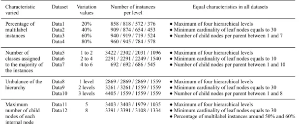
TABLE4. Variations Performed in the Datasets Generated.
Characteristic Dataset Variation Number of instances Equal characteristics in all datasets
varied values per level
Percentage of Data1 20% 858 / 818 / 572 / 376 Maximum of four hierarchical levels
multilabel Data2 40% 909 / 874 / 654 / 453 Minimum cardinality of leaf nodes equals to 30
instances Data3 60% 940 / 919 / 719 / 524 Number of child nodes per parent between 1 and 7
Data4 80% 960 / 945 / 784 / 578
Number of Data5 1 to 2 3422 / 2302 / 2031 / 1096 Maximum of four hierarchical levels
classes assigned Data6 2 to 4 2291 / 2291 / 2249 / 1540 Minimum cardinality of leaf nodes equals to 10
to the majority of Data7 4 to 6 692 / 692 / 686 / 545 Number of child nodes per parent between 1 and 10
the instances
Unbalance of the Data8 1 level 2869 / 2869 / 2869 / 1559 Maximum of four hierarchical levels
hierarchy Data9 2 levels 3261 / 3261 / 1559 / 1559 Minimum cardinality of leaf nodes equals to 30
Data10 3 levels 4405 / 1559 / 1559 / 1559 Number of child nodes per parent between 1 and 8
Maximum Data11 5 3403 / 3403 / 1979 / 1035 Maximum of four hierarchical levels
number of child Data12 8 3391 / 3391 / 3108 / 1334 Minimum cardinality of leaf nodes equals to 30
nodes of each Percentage of multilabel instances around 50% and 60%
internal node
classes and still keeping a sufficient number of instances with the same label cardinalities for training.
As another example of the difficulty in generating many datasets from a specific real-world one, consider the task of generating a dataset with 10% of its instances assigned to
a class A, 20% of its instances assigned to a classB, 30% of its instances assigned to a
classC, and 40% of its instances assigned to a classD. Let us consider also that we need
to (i) keep the label cardinality of the instances unchanged, (ii) ensure that all instances are classified in the last hierarchy level in order to obtain a complete level balance, and (iii) ensure that all internal nodes have a specific number of child nodes. Hence, although we preserve as much as possible the original characteristics of the dataset, sometimes varying one characteristic inevitably changes another. Despite this difficulty, overall, the generated datasets are useful to show how different hierarchical and multilabel variations influence the different classification methods and evaluation measures.
Table 4 shows the variations investigated and the datasets generated. The first two char-acteristics varied (shown in the first column of the table) are multilabel charchar-acteristics, whereas the last two are hierarchical characteristics. The first dataset variation was the per-centage of multilabel instances in the dataset. It is important to study the effect of this variation because, in general, the larger the number of instances having more than one class label, the more difficult the multilabel classification problem is. Four values were considered for this characteristic: 20%, 40%, 60%, and 80% of multilabel instances.
To generate the datasets Data1, Data2, Data3, and Data4, all instances from the original dataset, which respected the constraints shown in Table 4, were selected. Table 5 shows, for each of the datasets, the distribution of the classes over the instances.
The second characteristic varied was the number of classes assigned to the majority of the instances. Three alternative values were considered: datasets with the majority of their instances assigned to 1 to 2, 2 to 4, and 4 to 6 classes. Varying the values of this char-acteristic is important because, in principle, different numbers of classes per instance will result in different values of predictive performance measures, such as hierarchical precision and hierarchical recall. More precisely, as the number of classes per instance increases, one would expect precision to increase (there is a higher chance that a predicted class is really a true class simply because the instance has more true classes) and recall to decrease (there is a higher chance that a true class is not predicted only because there are more true classes).
TABLE5. Distribution of Classes Over the Instances When Varying the Percentage of Multilabel Instances.
Data1 661 129 53 11 2 1 1 1 2 3 4 5 6 7 Data2 521 241 106 28 9 2 1 1 1 2 3 4 5 6 7 8 Data3 355 360 161 45 15 2 1 1 1 2 3 4 5 6 7 8 Data4 178 485 209 64 18 4 1 1 1 2 3 4 5 6 7 8
For each dataset, the first row shows the number of instances assigned to the number of classes shown in the second row.
TABLE6. Distribution of Classes Over the Instances When Varying the
Number of Classes Assigned to the Majority of the Instances.
Data5 2521 901 1 2 Data6 91 1155 727 218 1 2 3 4 Data7 18 34 132 287 141 80 1 2 3 4 5 6
For each dataset, the first row shows the number of instances assigned to the number of classes shown in the second row.
To generate the Data5 dataset, all instances with 1 or 2 labels, respecting the constraints described in Table 4, were selected from the original dataset (2521 instances with 1 class and 901 instances with 2 classes). Because of the difficulties previously described for the generation of the datasets, it was not possible to generate datasets with all instances assigned to 2 to 4 classes and to 4 to 6 classes respecting all constraints described in Table 4. All the instances were randomly selected from the original dataset. Table 6 shows, for each dataset, the distribution of the classes over the instances. It is possible to see that, as desired, we varied the multilabel characteristic for all datasets.
Different levels of hierarchy unbalance were also tested, using 1, 2, and 3 levels of unbalance. This characteristic was varied because it can have a large influence on the per-formances of the classification methods. It is expected that as the hierarchy becomes more unbalanced, the divide and conquer mechanism of the local methods is affected. As the global methods deal with all classes at the same time, it is also interesting to see how unbalanced hierarchies influence their predictive performance.
To vary the unbalance of the hierarchies, complete trees were generated, where each instance is classified into a leaf node. As can be seen in the fourth column of Table 4, as Data8 is one level unbalanced, all the instances reach the third level, and just some instances reach the fourth hierarchical level. The same happens for the Data9 and Data10 datasets. Again, all instances from the original dataset respecting the constraints shown in
TABLE7. Distribution of Classes Over the Instances When Varying the Unbalance of the Hierarchy. Data8 1421 786 420 146 77 14 4 1 1 2 4 4 5 6 7 10 Data9 1496 873 507 231 93 43 13 3 1 1 1 2 3 4 5 6 7 8 9 11 Data10 2803 905 393 181 89 27 5 2 1 2 3 4 5 6 7 8
For each dataset, the first row shows the number of instances assigned to the number of classes shown in the second row.
TABLE8. Distribution of Classes Over the Instances When Varying the Maximum Number of Child Nodes
per Internal Node.
Data11 1675 953 472 196 69 29 5 3 1
1 2 3 4 5 6 7 8 9
Data12 1612 1236 620 297 97 38 26 2 2 1
1 2 3 4 5 6 7 8 9 10
For each dataset, the first row shows the number of instances assigned to the number of classes shown in the second row.
Table 4 were selected. Table 7 shows, for each dataset, the distribution of the classes over the instances.
Finally, datasets with a variation in the maximum number of children per internal node were generated, to have the majority of their nodes with 5 and 8 children. The increase in the number of children per internal node has a large influence on the number of leaf classes and on the number of multilabel instances, affecting the performance of the meth-ods. It is expected that the classification task becomes more difficult as the number of children is increased, harming the performance of the classification methods. The Data11 and Data12 datasets were generated similarly to the other datasets, by selecting all instances from the original dataset respecting the constraints presented in Table 4. Table 8 shows, for each dataset, the distribution of the classes over the instances, and Table 9 shows other characteristics of all the datasets generated.
Observing the statistics for the datasets, it is possible to see that there are some redun-dancies between them. It is possible to see that as the number of classes assigned to the majority of the instances is increased, the percentage of multilabel instances is also increased. As the number of classes in datasets Data5, Data6, and Data7 is increased from 1 to 2 until 4 to 6 classes per instance, the multilabel percentages of these datasets are 26.32% (1 to 2), 96.02% (2 to 4), and 97.39% (4 to 6). These redundancies occur only when the per-centage of multilabel instances is either small (26.32%) or too large (96.02% and 97.39%). The percentage variations adopted in the Data1, Data2, Data3, and Data4 datasets range from 20%, 40%, 60%, and 80%, allowing better insights regarding the performances of the methods and measures with more variations.
It is also possible to see a redundancy between the variations concerning the unbalance of the hierarchies and the maximum number of child nodes for each internal node. The multilabel percentages in the Data8, Data9, and Data10 datasets are 50.47%, 54.12%, and 36.36%, respectively, whereas the multilabel percentages in the Data11 and Data12 datasets
TABLE9. Characteristics of the Generated Datasets, Varying the Number of Multilabel Instances and the Characteristics of the Hierarchy.
No. of instances Average no. of instances per class Average no. of classes per instance
No. of No. of
Dataset attributes classes Total Multilabel L1 L2 L3 L4 L1 L2 L3 L4
Datasets varying the percentages of multilabel instances
Data1 77 135 858 197 57.20 20.97 13.61 9.64 1.20 1.21 0.90 0.72
Data2 77 139 909 388 60.60 22.41 14.53 11.32 1.43 1.49 1.13 0.92
Data3 77 139 940 585 62.66 23.56 15.97 13.10 1.65 1.76 1.29 1.02
Data4 77 139 960 782 64.00 24.23 17.42 14.45 1.85 2.01 1.45 1.02
Datasets varying the numbers of classes assigned per instance
Data5 77 163 3422 901 228.13 50.04 29.86 32.23 1.21 1.34 1.15 0.77
Data6 77 235 2291 2200 134.76 40.19 22.04 26.10 2.14 2.32 2.01 1.16
Data7 77 236 692 674 40.70 12.14 6.66 9.23 3.22 3.68 3.10 1.65
Datasets varying the levels of unbalance in the hierarchies
Data8 77 181 2869 1448 204.92 89.65 45.53 21.65 1.53 1.66 1.78 1.41
Data9 77 159 3261 1765 232.92 101.90 38.02 21.65 1.70 1.91 1.26 1.41
Data10 77 147 4405 1602 314.64 77.95 38.02 21.65 1.54 1.20 1.26 1.41
Datasets varying the maximum numbers of children per internal node
Data11 77 198 3403 1728 226.86 83.00 28.27 14.37 1.49 1.71 1.23 1.02
Data12 77 206 3931 2319 262.06 89.34 41.44 18.52 1.59 1.85 1.47 0.60
are, respectively, 50.77% and 58.99%. Despite these redundancies, the number of child nodes for each node in the Data8, Data9, and Data10 datasets did not suffer much variation, whereas in the Data11 and Data12 datasets this variation was higher.
The next sections present the results for all dataset variations considering different mea-sures and methods. There are a few observations that hold for all graphs plotted from now on. In Figures 6, 7, 8, and 9, the values of the predictive performance evaluation measures are divided into two types of graphs: on the left column, we always report precision-related measures plus the hierarchical loss, and on the right column are reported the recall-related measures. These figures are also divided into four parts—denoted (a), (b), (c), and (d)— each of them representing results for one specific method. The reader may also note that the values reported may be considered considerably low for standard classification applications. However, in hierarchical multilabel datasets, this is quite common, given the difficulty of the tasks being solved.
Figures 10, 11, 12, and 13 present the values considering the F-measure variations. Each figure is divided in four parts—(a), (b), (c), and (d)—each of them representing the F-measure results for a specific method.
It is important to point out that these graphs can be read in many different ways. Here, we focus on analyzing the behavior of the evaluation measures when used with different datasets’ characteristics and different HMC methods. We analyze how the performance of different HMC methods is affected by the use of different evaluation measures or dataset characteristics, and we compare the performances of the global and local classification approaches based on the measures investigated.
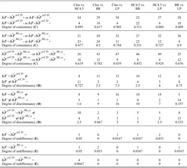
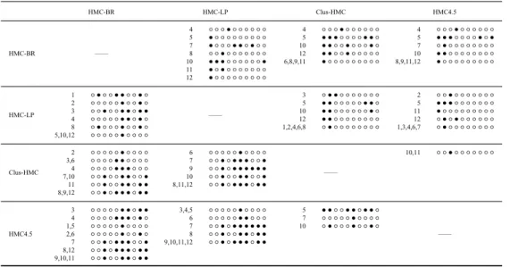
We also compared the evaluation measures considering their degrees of consistency, discriminancy, and indifferency, as suggested by Huang and Ling (2005). The results of these comparisons are shown in Tables 10, 11, and 12. Because of space restrictions, in the tables, we represented the methods Clus-HMC, HMC4.5, HMC-BR and HMC-LP as, respectively, Clus, HC4.5, BR and LP.
(a) HMC-BR method
(b) HMC-LP method
(c) HMC4.5 method
(d) Clus-HMC method
Approximate Multilabel Percentage
Approximate Multilabel Percentage
Approximate Multilabel Percentage
Approximate Multilabel Percentage Approximate Multilabel Percentage
Approximate Multilabel Percentage Approximate Multilabel Percentage Approximate Multilabel Percentage
Measures’ Values Measures’ Values
Measures’ Values Measures’ Values Measures’ Values 20% 40% 60% 80% 0.05 0.10 0.15 H Precision H Micro Precision H Macro Precision H Loss Function 20% 40% 60% 80% 0.02 0.04 0.06 0.08 0.1 0 H Recall H Micro Recall H Macro Recall Measures’ Values 20% 40% 60% 80% 0.02 0.04 0.06 0.08 0.10 0.12 0.14 H Precision H Micro Precision H Macro Precision H Loss Function 20% 40% 60% 80% 0.02 0.04 0.06 0.08 0.10 0.12 0.14 H Recall H Micro Recall H Macro Recall Measures’ Values 20% 40% 60% 80% 0.02 0.04 0.06 0.08 0.10 0.12 H Precision H Micro Precision H Macro Precision H Loss Function 20% 40% 60% 80% 0.05 0.10 0.15 H Recall H Micro Recall H Macro Recall Measures’ Values 20% 40% 60% 80% 0.02 0.04 0.06 0.08 0.10 0.12 0.14 H Precision H Micro Precision H Macro Precision H Loss Function 20% 40% 60% 80% 0.02 0.04 0.06 0.08 0.10 0.12 0.14 H Recall H Micro Recall H Macro Recall
Number of Classes Assigned to the Majority of the Instances Measures’ Values 1 to 2 2 to 4 4 to 6 0.00 0.05 0.10 0.15 0.20 H Precision H Micro Precision H Macro Precision H Loss Function
Number of Classes Assigned to the Majority of the Instances Measures’ Values 1 to 2 2 to 4 4 to 6 0.05 0.10 0.15 0.20 H Recall H Micro Recall H Macro Recall (a)HMC-BR method
Number of Classes Assigned to the Majority of the Instances Measures’ Values 1 to 2 2 to 4 4 to 6 0.05 0.10 0.15 H Precision H Micro Precision H Macro Precision H Loss Function
Number of Classes Assigned to the Majority of the Instances Measures’ Values 1 to 2 2 to 4 4 to 6 0.05 0.10 0.15 H Recall H Micro Recall H Macro Recall (b)HMC-LP method
Number of Classes Assigned to the Majority of the Instances Measures’ Values 1 to 2 2 to 4 4 to 6 0.05 0.10 0.15 0.20 0.25 H Precision H Micro Precision H Macro Precision H Loss Function
Number of Classes Assigned to the Majority of the Instances Measures’ Values 1 to 2 2 to 4 4 to 6 0.05 0.10 0.15 0.20 0.25 0.30 H Recall H Micro Recall H Macro Recall (c)HMC4.5 method
Number of Classes Assigned to the Majority of the Instances Measures’ Values 1 to 2 2 to 4 4 to 6 0.05 0.10 0.15 0.20 0.25 H Precision H Micro Precision H Macro Precision H Loss Function
Number of Classes Assigned to the Majority of the Instances Measures’ Values 1 to 2 2 to 4 4 to 6 0.05 0.10 0.15 0.20 0.25 H Recall H Micro Recall H Macro Recall (d)Clus-HMC method
FIGURE7. Results for different evaluation measures varying the number of classes assigned to the majority
Level of Unbalance
Measures’ Values
1 level 2 levels 3 levels
0.05 0.10 0.15 H Precision H Micro Precision H Macro Precision H Loss Function Level of Unbalance Measures’ Values
1 level 2 levels 3 levels
0.02 0.04 0.06 0.08 0.10 0.12 0.14 H Recall H Micro Recall H Macro Recall (a) HMC-BR method Level of Unbalance Measures’ Values
1 level 2 levels 3 levels
0.05 0.10 0.15 H Precision H Micro Precision H Macro Precision H Loss Function Level of Unbalance Measures’ Values
1 level 2 levels 3 levels
0.05 0.10 0.15 H Recall H Micro Recall H Macro Recall (b) HMC-LP method Level of Unbalance Measures’ Values
1 level 2 levels 3 levels
0.02 0.04 0.06 0.08 0.10 0.12 0.14 H Precision H Micro Precision H Macro Precision H Loss Function Level of Unbalance Measures’ Values
1 level 2 levels 3 levels
1 level 2 levels 3 levels 1 level 2 levels 3 levels
0.05 0.10 0.15 0.20 H Recall H Micro Recall H Macro Recall (c) HMC4.5 method Level of Unbalance Measures’ Values 0.02 0.04 0.06 0.08 0.10 0.12 0.14 H Precision H Micro Precision H Macro Precision H Loss Function Level of Unbalance Measures’ Values 0.05 0.10 0.15 0.20 H Recall H Micro Recall H Macro Recall (d) Clus-HMC method
5 children 8 children 0.05 0.10 0.15 0.20 H Recall H Micro Recall H Macro Recall Measures’ Values Measures’ Values Measures’ Values Measures’ Values Measures’ Values Measures’ Values Measures’ Values Measures’ Values 5 children 8 children 0.05 0.10 0.15 0 .20 H Precision H Micro Precision H Macro Precision H Loss Function (a) HMC-BR method 5 children 8 children 0.05 0.10 0.15 H Recall H Micro Recall H Macro Recall 5 children 8 children 0.05 0.10 0.15 0.20 H Precision H Micro Precision H Macro Precision H Loss Function (b) HMC-LP method 5 children 8 children 0.05 0.10 0.15 H Precision H Micro Precision H Macro Precision H Loss Function 5 children 8 children 0.05 0.10 0.15 0.20 0.25 H Recall H Micro Recall H Macro Recall (c) HMC4.5 method
Maximum Number of Children Maximum Number of Children
Maximum Number of Children Maximum Number of Children
Maximum Number of Children Maximum Number of Children
Maximum Number of Children Maximum Number of Children
5 children 8 children 0.05 0.10 0.15 H Precision H Micro Precision H Macro Precision H Loss Function 5 children 8 children 0.05 0.10 0.15 0.20 0.25 H Recall H Micro Recall H Macro Recall (d) Clus-HMC method
FIGURE9. Results for different evaluation measures varying the maximum number of child nodes of each