Rejection and Online Learning with
Prototype-based Classifiers in
Adaptive Metrical Spaces
Lydia Fischer
Dissertation
vorgelegt zur Erlangung des Grades
Doktor der Naturwissenschaften (Dr. rer. nat.)
Disputation am 23. September 2016
Third Examiner: Prof. Dr. Thomas Martinetz, L ¨ubeck University, Germany Printed on non-ageing paper according to ISO 9706.
Bielefeld University – Faculty of Technology P.O. Box 10 01 31
D-33501 Bielefeld, Germany
Lydia Fischer
CorLab – Research Institute for Cognition and Robotics Theoretical Computer Science Research Group
Abstract
The rising amount of digital data, which is available in almost every domain, causes the need for intelligent, automated data processing. Classification models constitute particularly popular techniques from the machine learning domain with applications ranging from fraud detection up to advanced image classification tasks. Within this thesis, we will focus on so-called prototype-based classifiers as one prominent family of classifiers, since they offer a simple classification scheme, interpretability of the model in terms of prototypes, and good generalisation performance. We will face a few crucial questions which arise whenever such classifiers are used in real-life scenarios which require robustness and reliability of classification and the ability to deal with complex and possibly streaming data sets. Particularly, we will address the following problems:
• Deterministic prototype-based classifiers deliver a class label, but no confi-dence of the classification. The latter is particularly relevant whenever the costs of an error are higher than the costs to reject an example, e. g., in a safety critical system. We investigate ways to enhance prototype-based classifiers by a certainty measure which can efficiently be computed based on the given classifier only and which can be used to reject an unclear classification.
• For an efficient rejection, the choice of a suitable threshold is crucial. We investigate in which situations the performance of local rejection can surpass the choice of only a global one, and we propose efficient schemes how to optimally compute local thresholds on a given training set.
• For complex data and lifelong learning, the required classifier complexity can be unknown a priori. We propose an efficient, incremental scheme which adjusts the model complexity of a prototype-based classifier based on the certainty of the classification. Thereby, we put particular emphasis on the question how to adjust prototype locations and metric parameters, and how to insert and/or delete prototypes in an efficient way.
• As an alternative to the previous solution, we investigate a hybrid architecture which combines an offline classifier with an online classifier based on their certainty values, thus directly addressing the stability/plasticity dilemma. While this is straightforward for classical prototype-based schemes, it poses
some challenges as soon as metric learning is integrated into the scheme due to the different inherent data representations.
• Finally, we investigate the performance of the proposed hybrid prototype-based classifier within a realistic visual road-terrain-detection scenario.
Thanks . . .
. . . to my encouraging supervisors who had a main impact on my development as PhD student and the work I did.
. . . to Dr. Heiko Wersing.
. . . to Prof. Dr. Barbara Hammer. . . . to my proofreaders of the thesis.
. . . to the Honda Research Institute (HRI-EU) for funding the PhD project giving me this great opportunity.
. . . to my friends at the Honda Research Institute for a great time, fruitful discus-sions, and your support.
. . . to my friends at the Technical Computer Science Group at Bielefeld University for great conference trips, dinners, and jam sessions . . . we rocked ;-) . . . to my friends at the Computational Intelligence Group at Mittweida University
of applied sciences. . . . to my family.
Contents
1. Introduction 1
1.1. Motivation . . . 1
1.2. Contribution of this Thesis . . . 3
1.3. Structural Overview of this Thesis . . . 4
1.4. Publications and Funding Related to this Thesis . . . 5
2. Principles of Rejection 7 2.1. General Setting . . . 8
2.2. Evaluation of Reject Options . . . 11
2.3. State of the Art Approaches . . . 15
2.4. Conclusion . . . 20
3. Prototype-based Classification 21 3.1. Generalised Learning Vector Quantisation . . . 23
3.2. Generalised Matrix Learning Vector Quantisation . . . 24
3.3. Localised Generalised Matrix Learning Vector Quantisation . . . . 26
3.4. Robust Soft Learning Vector Quantisation . . . 26
4. Global Reject Option 29 4.1. Motivation . . . 29
4.2. Research Questions . . . 30
4.3. Certainty Measures . . . 30
4.3.1. Bayes . . . 31
4.3.2. Conf . . . 31
4.3.3. RelSim – The Relative Similarity . . . 32
4.3.4. Dist . . . 32
4.3.5. d+ . . . 34
4.3.6. Comb . . . 34
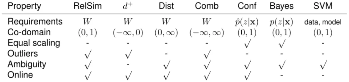
4.3.7. Characteristics of the Certainty Measures . . . 34
4.4. Experiments for Global Rejection . . . 36
4.4.1. Artificial and Benchmark Data . . . 36
4.4.2. Results . . . 37
4.4.3. Summary of the Main Findings . . . 41
4.5. Comparison with Probabilistic Approaches . . . 42
4.5.1. Gaussian Mixture Model and its Certainty Measure . . . 42
4.5.2. Experiments . . . 43
4.5.3. Conclusion with Respect to Probabilistic Approaches . . . 46
4.6. Conclusion: Answering the Research Questions . . . 47
5. Local Reject Option 49 5.1. Motivation . . . 49
5.2. Research Questions . . . 50
5.3. Classifiers . . . 50
5.3.1. Prototype-based Classifiers . . . 50
5.3.2. Basic Decision Trees for Classification . . . 51
5.3.3. Support Vector Machine for Classification . . . 52
5.4. Local Rejection . . . 52
5.4.1. Certainty Measures . . . 53
5.4.2. Local Reject Option . . . 54
5.5. Optimal Choices of Rejection Thresholds . . . 56
5.5.1. Extended Pareto Front . . . 56
5.5.2. Optimal Global Rejection . . . 57
5.5.3. Optimal Local Rejection . . . 58
5.5.4. Formulation as Multiple Choice Knapsack Problem . . . 59
5.5.5. Local Threshold Adaptation by Dynamic Programming . . . 59
5.5.6. Local Threshold Adaptation by an Efficient Greedy Strategy 61 5.6. Experiments for Local Rejection . . . 62
5.6.1. Data Sets . . . 62
5.6.2. Dynamic Programming versus Greedy Optimisation . . . . 62
5.6.3. Experiments on Artificial Data . . . 63
5.6.4. Experiments on Benchmarks . . . 65
5.6.5. Medical Application – The Adrenal Tumours Data . . . 65
5.7. Conclusion: Answering the Research Questions . . . 67
6. Incremental Online Learning Vector Quantisation 69 6.1. Motivation . . . 69
6.2. Research Questions . . . 70
6.3. Related Work . . . 70
6.4. Incremental Online Learning Vector Quantisation . . . 72
6.5. Experiments . . . 75
6.5.1. Influence of Parameters for Incremental Learning . . . 76
6.5.2. Compatibility with Metric Learning . . . 77
6.5.3. Comparative Evaluation . . . 77
Contents ix
7. Combined Offline and Online Learning 81
7.1. Motivation . . . 81
7.2. Description of the Scenario . . . 83
7.3. Research Questions . . . 84
7.4. Related Work . . . 84
7.5. Combining Offline and Online Learning . . . 85
7.6. Experiments on Artificial and Benchmark Data . . . 87
7.7. Summary of the Main Findings . . . 96
7.8. Online Metric Learning for an Adaptation to Confidence Drift . . . . 97
7.9. Conclusion: Answering the Research Questions . . . 105
8. Application on Road Terrain Detection 107 8.1. Motivation . . . 107
8.2. Research Questions . . . 108
8.3. Road Terrain Detection – Related Work . . . 108
8.4. The Road Terrain Detection System . . . 110
8.5. The Scenario . . . 111
8.6. Experimental Studies . . . 112
8.7. Conclusion: Answering the Research Questions . . . 115
9. Conclusion 117 A. Appendix 121 A.1. Publications in the Context of this Thesis . . . 121
A.2. Data Properties . . . 123
A.3. Algorithms . . . 124
List of Tables
4.1. Properties of the studied certainty measures . . . 35
5.1. Sample rejects for three partitions and their losses and gains . . . 58
6.1. Comparison of several online, incremental LVQ approaches . . . . 70
6.2. Results of the ioLVQ and an incremental SVM . . . 78
7.1. Comparison of Queißer’s architecture and the OOL architecture . . 90
7.2. The different incremental LVQ approaches . . . 91
7.3. The parameters of the used approaches . . . 92
7.4. Results of the different lifelong learning architectures . . . 93
7.5. Parameters of the offline and the online classifiers . . . 103
7.6. The results of the Chequerboard data . . . 103
7.7. The results of the Blossom and the benchmark data . . . 104
A.1. Data properties . . . 123
List of Figures
1.1. Structural overview of this thesis . . . 4
2.1. Challenges in classification . . . 8
2.2. Rejection process . . . 8
2.3. Optimal reject option . . . 10
2.4. Optimal local reject option . . . 11
2.5. Examples of accuracy-reject-curves . . . 12
2.6. Ak-nearest neighbour certainty measure . . . 17
2.7. Our taxonomy for rejection . . . 19
3.1. Development of learning vector quantisation . . . 22
3.2. Scheme of quantities used in generalised learning vector quantisation 23 4.1. Contour lines of the certainty measures for an artificial 2D data . . 31
4.2. Dist in case of multiple prototypes per class . . . 33
4.3. Accuracy-reject-curves on Gaussian clusters . . . 37
4.4. Accuracy-reject-curves on benchmark data . . . 38
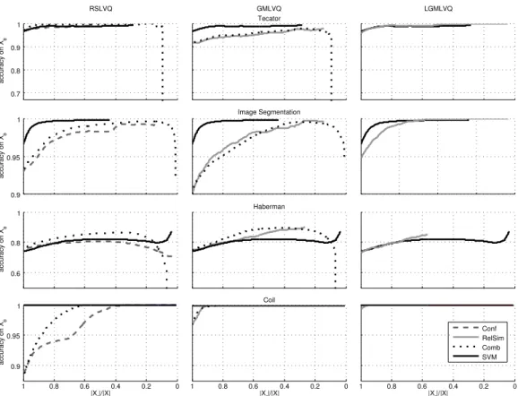
4.5. Comparison against the accuracy-reject-curves of the SVM . . . . 40
4.6. Accuracy-reject-curves of the comparison to probabilistic approaches 45 5.1. An exemplary decision tree with its partitions of the input space . . 51
5.2. Several certainty measures . . . 53
5.3. Example where a global reject option fails . . . 55
5.4. Example of losses/gains for a partition of the space . . . 57
5.5. Results of dynamic programming versus the greedy algorithm . . . 63
5.6. Results of local rejection for artificial data . . . 64
5.7. Results of local rejection for benchmark data . . . 66
5.8. Results for the medical adrenal tumours data set . . . 67
6.1. Scheme of machine learning scenarios . . . 71
6.2. Scheme of error-based prototype insertion . . . 74
6.3. Scheme of prototype deletion . . . 74
6.4. The Outdoor data set . . . 75
6.5. Different perspectives of an object of the Outdoor data set . . . 75
6.6. Effect of the parameters of ioLVQ . . . 76
6.7. Effect of the initialisation of the metric . . . 77
6.8. Comparison of ioLVQ in several settings . . . 79
6.9. Comparison of ioLVQ in several settings with an incremental SVM 79 7.1. A possible application scenario . . . 84
7.2. Two different types of lifelong learning architectures . . . 84
7.3. An architecture combining an online and an offline classifier . . . . 85
7.4. The Blossom data set . . . 87
7.5. A possible split in offline and online data of the Outdoor data . . . 88
7.6. A 2D visualisation of the Outdoor data set . . . 89
7.7. General data split in offline and online data . . . 90
7.8. The Chequerboard data set . . . 97
7.9. The settings of the Chequerboard data . . . 98
7.10.The desired partitioning of setting A and B . . . 98
7.11.Explanation of the result figures . . . 99
7.12.Exemplary results without confidence drift adaptation . . . 100
7.13.Scheme of OOL extension for confidence drift adaptation . . . 101
7.14.Exemplary results of the architecture with confidence drift adaptation102 7.15.The results of the Chequerboard data for three settings . . . 104
8.1. Data labelling through human driving . . . 109
8.2. Examples for road-like area and semantic road . . . 110
8.3. The algorithmic steps of the road terrain detection system . . . 111
8.4. How the system collects ground truth data . . . 111
8.5. Scheme of the used scenario . . . 112
8.6. Offline GMLVQ performance when features are removed . . . 113
8.7. GMLVQ road classification on exemplary images . . . 114
Abbreviations and Symbols
Abbreviationsk-NN k-nearest neighbour classifier ARC accuracy-reject-curve
CFE catastrophic forgetting effect
DP dynamic programming
GLVQ generalised learning vector quantisation GMLVQ generalised matrix learning vector quantisation GMM Gaussian mixture model
ioLVQ incremental online learning vector quantisation iSVM incremental support vector machine
LGMLVQ localised generalised matrix learning vector quantisation LVQ learning vector quantisation
NNC nearest neighbour classifier
OOL combined offline and online learning RSLVQ robust soft learning vector quantisation RTDS road terrain detection system
SVM support vector machine Classifier variables
αj a leaf of a decision tree
η(w) accumulated certainty values of classifications of points in the Voronoi cell represented byw
Γ the decision border induced by the decision tree gmax maximum storage capacity ofS
ˆ
p(·) estimated probability
Λ global matrix ofdΛ
Ω square root ofΛ
Ω(l, k) single element in thel-th row and thek-th column ofΩ Φ(·) a monotone increasing function
rnum In periods ofrnumseen training data points, it is checked if prototypes should be removed. σ variance of a Gaussian ε learning rate | · | cardinality of a set w a prototype
w± closest prototype of the same class/a different class with respect to a data point
x a data point
x(l),w(l),[·]l l-th element of a vector
ξ number of prototypes
ζ number of the partitions of the input space ζ number of the partitions of the input space cj label of prototypewj
d(·) dissimilarity measure
d± dissimilarity of a data point to the closest prototype of the same/of a different class
dΛj(·) dissimilarity measure of LGMLVQ dΛ(·) dissimilarity measure of GMLVQ E... cost function of . . .
M dimension of data, prototypes p(·) a probability
S set of wrongly classified data points Vj Voronoi cell of prototypewj
W set of prototypes
X a set of data points
yi class label of data pointxi
Z number of classes
Rejection
Eθj true rejects inΥj
Eθ true rejects: rejected data points which would be classified wrongly
Lθj false rejects inΥj
Lθ false rejects: rejected data points which would be classified correctly
Xθj rejected points inΥj
Abbreviations and Symbols xvii
opt(n, j, i) It measures the maximum number of true rejects obtained with n false rejects, and a restricted threshold vector (see 59).
θθθ threshold vector (local thresholds) θθθ threshold vector (local thresholds)
Θ the set of thresholds corresponding to correctly classified points θ threshold for rejection
Θj the set of thresholds corresponding to correctly classified points with
respect toΥj
θj local threshold, responsible forΥj
Υj Thej-th partition of the input space, e. g., a Voronoi cell.
E set of wrongly classified data points, errors Ej set of wrongly classified data points, errors inΥj
L set of correctly classified data points Lj set of correctly classified data points inΥj
r(·) certainty measure Xθj accepted points inΥj
1. Introduction
Chapter overview In this chapter, we first motivate the tackled topics of this thesis. Thereafter we give a structural overview of the single chapters.
1.1. Motivation
Digitalisation is progressing in many domains like in industrial applications with regard to industry 4.0, in biomedicine, personalisation, and driver assistance systems. This leads to a huge amount of data. Inspection and handling of gathered data make automated data analysis more and more important, since an analysis of the data could hardly be done by humans in an acceptable time frame. Machine learning and related research areas1provide techniques to extract structures or information automatically from available data.
These techniques are either supervised or unsupervised2. If information is available which groups data into a finite number of classes, a supervised technique can be applied. Unsupervised techniques deal with data without such information. For supervised machine learning, one aim is to extract characteristics of the classes and to identify where classes differ and what they have in common, respectively. One of the most popular principles to reach this aim is classification. The learning techniques used for classification have a basic principle in common: they want to minimise the number of errors in classification since they cause costs. Depending on the application these costs range between low (not critical) and huge (very critical, e. g., in the biomedical domain or safety related applications). One realisation of this principle which puts a particular emphasis on its gener-alisation ability, is based on maximising the margin between classes. Popular representatives are support vector machines (SVM, Boser et al., 1992) and learn-ing vector quantisation (LVQ, Kohonen, 1989). LVQ constitutes a prototype-based technique, and it will play a central role in this thesis as classification scheme. Another basic idea is to combine many weak classifiers into one powerful classifier,
1
These areas are for instance data analysis, computational intelligence, neural computation, pattern recognition, and statistical modelling. They aim at automatically extracting information from given data.
2
We are aware of finer grained subgroups as for instance semi-supervised techniques. Since we only use supervised techniques, we only distinguish these two groups.
to a so-called ensemble classifier. Random forests belong to ensemble classi-fier and they consist of several decision trees. This classiclassi-fier is suited for large data sets due to its short training time and its very efficient classification scheme. Neural networks are classifiers which are inspired by the human brain. They try to mimic the functionality of the brain. Lately they got popular with deep neural networks which are a powerful tool for classification, but the classifier is complex and the internal mechanisms are hard to interpret. There are classifiers based on probabilistic modelling as well, e. g., the Bayes classifier. They aim at estimating the class densities, e. g., with Gaussian distributions. Later, we will deal mainly with LVQ schemes as a typical classification techniques in this thesis because of their simple classification scheme and interpretable classification models. In chapter 3, we will explain the used LVQ schemes within this thesis as well as the concept of metric learning.
Since wrong classifications can have severe effects, a certainty information can be at least as important as the classification itself. Depending on the application, it can be better to reject a classification instead of making a mistake. Hence a reject can have lower costs than a false classification. Supervised techniques based on a probabilistic data modelling include such certainty information. The estimated probabilities of a data point belonging to a specific class can be used for this purpose. A low probability value can lead to rejection since the classification is uncertain. In chapter 4 we will discuss rejection based on probabilities. Techniques lacking such information can be enhanced with a statistical modelling on top or with certainty information based on heuristics, e. g., statistics of the neighbourhood or on distances. Using rejection comes along with the issue of choosing a suited certainty measure and a threshold judging an uncertain decision. More sophisti-cated rejection strategies use multiple thresholds, e. g., class-wise or even more fine-grained partitioning of the data. In chapter 4 we discuss several certainty measures suited for prototype-based classifiers and it also analyses rejection with one global threshold. The analysis of strategies with multiple thresholds can be found in chapter 5. There we also provide techniques which determine the best possible thresholds for a given setting.
Besides the hot topic of rejection, the area of lifelong machine learning gets more and more important (Polikar and Alippi, 2014). A recent definition states: ”Lifelong Machine Learning, or LML, considers systems that can learn many tasks over a lifetime from one or more domains. They efficiently and effectively retain the knowledge they have learned and use that knowledge to more efficiently and effectively learn new tasks (Silver et al., 2013).” Hence, approaches usable for lifelong learning have to deal with various issues. They have to be flexible such that including new content is possible (plasticity). Contrarily, already known information has to be maintained for later use (stability). The trade-off between those two
1.2. Contribution of this Thesis 3
principles is known as stability plasticity dilemma (Grossberg, 1980). To our knowledge there exists no satisfying solution for this dilemma in machine learning. However, the human brain seems to have a very efficient solution. Some of its working principles are explored and serve as inspiration for machine learning techniques with promising results (see, e. g., Kirstein et al., 2005, 2009, 2012). Ongoing research studies how these mechanisms operate and how to use them in lifelong machine learning. In chapter 6 and 7, we will extend and merge existing lifelong learning approaches in order to combine their advantages and to improve their behaviour regarding the stability plasticity dilemma. With our approaches, we focus on lifelong adaptability of the classifier complexity for LVQ schemes and on guaranteeing a minimal performance of a system by the combination of an offline and an online classifier.
1.2. Contribution of this Thesis
This thesis contains novel insights into the following questions:
• What are good deterministic certainty measures suitable for prototype-based classifiers and which properties do they have?
We investigate several deterministic certainty measures, e. g., the distance to the decision border. The analysed measures work well in almost all settings and they show a similar performance as probabilistic counterparts.
• Rejection can be based on a global threshold or on local thresholds which are valid in single partitions of the data space only. Which strategy should be applied in which setting and how can we choose best thresholds (global or local)?
Local thresholds are beneficial in settings where the data have local or class specific characteristics which are not captured by the used classifier. For settings with no local characteristics or with classifiers dealing with these characteristics, a global threshold suffices. We provide an optimal dynamic programming scheme and a fast greedy algorithm which determine the best thresholds on a given setting.
• Is it useful to integrate certainty information in lifelong learning architec-tures and is the powerful concept of metric adaptation (Bellet et al., 2013) compatible with this learning concept?
We show that the integration of certainty information in lifelong learning architectures is useful and that it can be combined with metric adaptation.
• Is it beneficial to transfer the concept of the discussed lifelong learning architecture to a real word application to improve its performance?
We exemplary test this for the road terrain detection system (RTDS, Fritsch et al., 2014). The system distinguishes between road and non-road in real traffic scenes. We show that a simple on-the-fly trained approach compared to the advanced RTDS provides reasonable results with some limitations. The next section contains the structure of this thesis and shortly recaps each chapter.
1.3. Structural Overview of this Thesis
state of the art rejection (chap. 2)
classification model (chap. 3)
extraction of certainty information (chap. 4)
global rejection (chap. 4)
local rejection (chap. 5)
online incremental learning (chap. 6)
combination with offline learning (chap. 7)
RTDS – application (chap. 8)
Figure 1.1.:Structural overview of this thesis (RTDS – road terrain detection system). The certainty information can either be used for rejection or for incremental learning.
The content of this thesis is visualised in Fig. 1.1. Each chapter of this thesis discusses one part of the figure in general.
Rejection strategies are the main focus of this thesis. We start with the intro-duction of basic rejection concepts and a literature overview in chapter 2. A reject option relaxes the constraint of a classifier to provide a class label in case of an uncertain decision. This way the classification of a data point is postponed and marked for further treatment. We establish the notation of global and local rejection and the theoretical framework for understanding and we discuss several existing rejection strategies. The literature survey enables us to point to relevant research topics which we tackle in chapter 4 and 5.
We present prototype-based classifiers and the later used LVQ schemes in chapter 3. We chose these classification technique due to its simple classification scheme, the interpretability of the classifiers and the lifelong learning suitability. But there are only few rejection strategies available for prototype-based classifiers such that we carry on the research in this important topic.
1.4. Publications and Funding Related to this Thesis 5
The focus of chapter 4 is global rejection, especially in the context of prototype-based classifiers. We present several dissimilarity-prototype-based certainty measures which are suited for this classifier type and we discuss their properties. Subsequently, we present results for global rejection based on those measures for artificial toy data and public benchmarks and we compare the results with probabilistic counterparts and a state of the art approach. Note that global rejection implicitly assumes an equally scaled certainty measure in the whole input space.
In chapter 5 we move on to the topic of local rejection which relaxes the implicit assumption of global rejection, since it relies on a partitioning of the input space only assuming a homogeneous scaling in each partition. We describe an optimal dynamic programming scheme and an efficient greedy scheme to determine the best parameters for local rejection. Since lots of classifiers provide a partitioning of the input space, we compare local and global rejection for several types of classifiers on artificial toy data and public benchmarks. Experiments on a medical data set highlight the usefulness in this domain.
Certainty measures indicate areas where a classifier tends to do mistakes. In chapter 6 we analyse weather certainty information can be used not only for rejection, but also in other machine learning areas, e. g., in lifelong learning. We use certainty information as criterion for inserting or deleting prototypes in a new online, incremental learning vector quantisation approach for lifelong learning. Additionally, this chapter contains an analysis of the parameters of the incremental classifier and an investigation of integrating different metric learning schemes. We report results for public benchmarks and one real-life robotic data set.
Chapter 7 contains the analysis of a different approach for lifelong learning which is an architecture combining the classifier from chapter 6 with a static offline trained one to avoid the so-called catastrophic forgetting effect. A dynamic classifier selection based on certainty values provided by the two classifiers defines the final output class label for a given input. We provide results of this architecture on artificial toy data, public benchmarks, and for real-life robotic data and we compare them to other lifelong learning methods.
So far we analysed lifelong learning approaches without a concrete application. A possible area of application could be the field of road terrain detection. Thus, we analyse in chapter 8 how good an online, trained prototype-based classifier can get in comparison to the offline trained road terrain detection system. Subsequently, we sum up the achieved knowledge and we point to future work in chapter 9.
1.4. Publications and Funding Related to this Thesis
The following articles have been published in the context of this thesis:
Journal articles
[J16] L. Fischer, B. Hammer, and H. Wersing. Optimal local rejection for classifiers. Neurocomputing,http://dx.doi.org/10.1016/j.neucom.2016.06.038, 2016. [J15] L. Fischer, B. Hammer, and H. Wersing. Efficient rejection strategies for
prototype-based classification. Neurocomputing, 169 (2015) 334-342.
Conference articles
[C16] L. Fischer, B. Hammer, and H. Wersing. Online Metric Learning for an Adaptation to Confidence Drift. InIJCNN, pages 748–755, 2016.
[C15b] L. Fischer, B. Hammer, and H. Wersing. Combining offline and online classifiers for life-long learning. InIJCNN, pages 2808–2815, 2015.
[C15a] L. Fischer, B. Hammer, and H. Wersing. Certainty-based prototype insertion/ deletion for classification with metric adaptation. InESANN, pages 7–12, 2015. [C14c] L. Fischer, B. Hammer, and H. Wersing. Local rejection strategies for learning
vector quantization. InICANN, pages 563–570, 2014.
[C14b] L. Fischer, D. Nebel, T. Villmann, B. Hammer, and H. Wersing. Rejection strategies for learning vector quantization – A comparison of probabilistic and deterministic approaches.3 InWSOM, pages 109–118, 2014.
[C14a] L. Fischer, B. Hammer, and H. Wersing. Rejection strategies for learning vector quantization. InESANN, pages 41–46, 2014.
Non-refereed publications
[TR16] L. Fischer, and T. Villmann. A Probabilistic Model with Adaptive Rejection. Machine Learning Reports, MLR-01-2016:1–19, 2016.
[TR15] L. Fischer, B. Hammer, and H. Wersing. Optimum Reject Options for Prototype-based Classification. CoRR, abs/1503.06549, 2015.
Funding acknowledgments
The following institutions and associated grants are gratefully acknowledged:
• TheCor-Lab Research Institute for Cognition and Roboticsin cooperation with the Honda Research Institute Europe.
2. Principles of Rejection
Chapter overview We introduce the basic concept of global and local rejection strategies and we give an overview on existing state of the art approaches which can be applied to several types of classifiers, e. g., probabilistic classifiers and support vector machines. It turns out that the literature is lacking adequate certainty measures for prototype-based classifiers and an analysis/comparison of them. Furthermore, there does not exist a comparison between global and local rejection strategies for different classifier types. Regarding local rejection, there is no approach for determining appropriate local thresholds for a given setting. Those weak points motivated our research which is described in the subsequent chapters.
Parts of this chapter are based on:
[J16] L. Fischer, B. Hammer, and H. Wersing. Optimal Local Rejection for Classifiers. Neurocomputing, submitted.
[J15] L. Fischer, B. Hammer, and H. Wersing. Efficient Rejection Strategies for Prototype-based Classifica-tion.Neurocomputing, 169 (2015) 334–342.
When creating a classifier, the main target is to achieve the best possible accuracy. In case of errors, one is interested in a mechanism indicating whether the decision of a classifier can be trusted (certain classification) or if the classifier is probably erring (uncertain classification) for a given input. Such a mechanism is especially important in applications where a wrong classification can have severe effects, e. g., in driver assistance systems or in the biomedical domain. Vailaya and Jain (2000) discuss two main reasons for uncertain classification (Fig. 2.1):
• Ambiguity: The classification of the data point is unclear, e. g., the point is close to a decision border, or it lies in a region with overlapping classes. • Outliers: The data point is dissimilar to any already seen data point, e. g., it
is caused by noise or it is an instance of a yet unseen class or cluster. A reject option can be used in order to decide if a classification is certain enough (Fig. 2.2). Rejected inputs can be marked for further tests or they can be passed to domain experts who will do a manual classification.
Based on such considerations, quite a few heuristic rejection strategies have been proposed (see e. g., Cordella et al., 1995; Vailaya and Jain, 2000; Fumera et al., 2000; Stefano et al., 2000; Fumera and Roli, 2002; Suutala et al., 2004). In the next section we explain the general setting and we give a mathematical formulation for rejection strategies.
outliers outliers
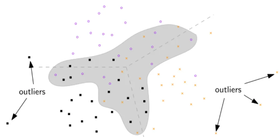
Figure 2.1.:Challenges in classification – A three class setting shows two main challenges in classification: overlapping classes and outliers (different symbols and colour indicate the class of the data points; the dashed lines indicate class borders and the grey area shows overlapping classes).
trained
classifier reject
accept assigned class label
reject decision
data point class label no
yes
Figure 2.2.:Rejection process: A trained classifier provides a class label for the given data point. If the criteria for rejecting the decision is fulfilled, the decision is rejected and otherwise the assigned class label is accepted.
2.1. General Setting
As stated previously, we consider multi-class classification problems with training data X = {(xi, yi) ∈ RM × {1, . . . , Z}}Ni=1, whereby data are drawn according to some unknown probability distribution P on RM × {1, . . . , Z}. A classifier
implements a functionc:RM → {1, . . . , Z}. For typical settings, a classifier aims
at minimising the classification error
E(c) := Z
L(c(x), y)dP(x, y).
WithL(c(x), y)denoting the 0-1-loss function
L(c(x), y) := (
0 ifc(x) =y 1 otherwise.
Since P is typically unknown, standard classification schemes often optimise the empirical error (2.1) instead, or a related, numerically simpler (e. g., convex)
2.1. General Setting 9 surrogate loss. ˆ E(c, X) := 1 N X 1≤i≤N L(c(xi), yi) (2.1)
For popular classifiers, results from computational learning theory guarantee that the empirical error allows us to uniformly bound the true error for i. i. d. data and a proper regularisation (Tewari and Bartlett, 2007).
A multi-class classifier can be extended by a reject option after training (Fig. 2.2). Hence, we assume a trained classifier is given. In addition to the output class, many classifiers provide a certainty measure of its classification like the class probability or the distance to the decision border. This fact is used whenever classification is extended by a reject option. Points with a bad certainty value are rejected since we consider reject options based on certainty measures where a higher value indicates higher certainty. Formally, a reject option extends the classifier to a mapping (denoted with the same symbol)c:RM → {1, . . . , Z, r},
where the symbol r denotes the rejection of the classification of inputxwhich is typically defined by an extended 0-1-loss function
L(c(x), y) := 0 ifc(x) =y b ifc(x) = r 1 ifc(x)6=y, c(x)6= r , (2.2)
where costsb∈(0,1)are assigned to a reject r (Bartlett and Wegkamp, 2008). As example, for driver assistance systems it is better to reject an uncertain decision instead of a classification which initiates a wrong interaction of the system possibly causing severe effects.
The definition (2.2) is similar to the early definition used by Chow (1970) who proposed an optimal rejection strategy in the sense of error reject trade-off when the true class probabilities are known. For valuesb <1, it is beneficial to reject a wrong classification rather than to provide a false output, but rejects always come at the risk of rejecting correctly classified points as well. Hence, the threshold (or threshold vector, discussed later on) starting from which rejection is done, is a crucial parameter. For settings with known class probabilities the optimal threshold can be obtained according to Chow (1970), but in general this information is unavailable. It is crucial to find an answer to the question how to choose thresholds which optimise the modified classification error. While threshold optimisation is straightforward in the case of one global threshold, the optimisation problem is more difficult for local rejection strategies as proposed in Fumera et al. (2000) and it will be discussed in chapter 5.
In the following, the basic concept and differences between global and local rejection are explained.
Global Rejection
Given a certainty measure:
r:RM →R,x7→r(x),
a data pointxand a thresholdθ∈R, a simple reject option is to rejectxiff
r(x)< θ .
If a data point is rejected, no classification takes place and the decision is post-poned. The data point is marked for further treatment. In most classical rejection strategies one global threshold value is taken, and an optimal value depends on the respective costs of misclassification versus reject. Since the thresholdθ is chosen uniformly for the whole input space, we denote such a reject option as global reject option. This implicitly assumes an equally scaled measure across the input space. For a true probability two conditions hold: (i) it is normalised, and (ii) equal probability values lead to an identical uncertainty of the classification, in-dependently of the location of the related data points. We say a certainty measure is equally scaled when both conditions hold. Though we will see promising results in section 4.4, we can construct situations where certainty measures violate these conditions (see section 5.4.2). Local threshold strategies relax this assumption.
As Vailaya and Jain (2000) mentioned, uncertainty can have two different reasons: data points being outliers, or data points being located in ambiguous regions. An optimal reject option would reject exclusively wrongly classified data points (Fig. 2.3). Of course in practice no certainty measure can fulfil this.
⇒
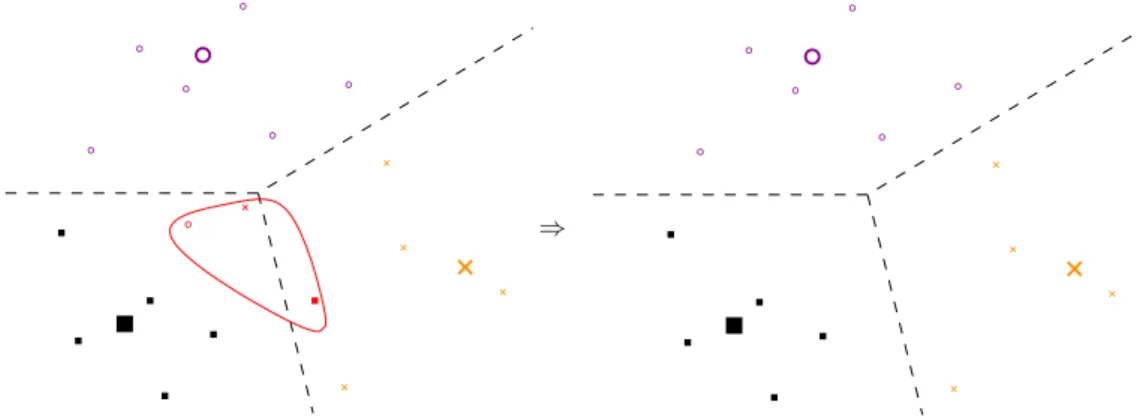
Figure 2.3.:Optimal reject option – Sketch of an artificial three-class setting (different symbols). The bigger symbols are the prototypes of the classifier. Left: no rejection; An optimal reject option rejects the red encircled errors only. Right: reject option is applied.
Local rejection strategies offer a finer grained control of rejection and the basic concept is explained in the following.
2.2. Evaluation of Reject Options 11
Local Rejection
A local threshold strategy relies on a given partition of the input spaceRM intoζ
disjunct, non-empty setsΥj such that
RM =
[
1≤j≤ζ
Υj .
Using a different thresholdθj in every setΥj enables a finer control of rejection
(Vailaya and Jain, 2000). A separate thresholdθj ∈Ris chosen for every setΥj,
and the reject option is given by a threshold vectorθθθ= (θ1, . . . , θζ)of dimensionζ
equal to the number of sets in the partition. A data pointxis rejected iff r(x)< θj wherex∈Υj .
Hence,θj determines the behaviour for the setΥj only. In the special case of one
regionΥjper classifier output classj, local thresholds realise class-wise rejection.
Figure 2.4 shows an instance of this local rejection strategy performing optimally if only labelling errors are rejected. In general this is not the case for local/global rejection strategies as mentioned before.
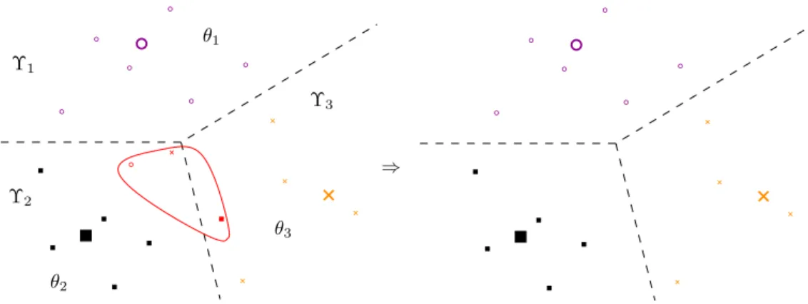
⇒ Υ1 Υ2 Υ3 θ1 θ3 θ2
Figure 2.4.:Optimal local reject option – Sketch of an artificial three-class setting (different symbols) with an prototype-based model. The bigger symbols are the prototypes of the classifier. It is the same plot as Fig. 2.3. New: There are three partitionsΥj and each one is associated with a single thresholdθj. Left: Model without rejection, three encircled points are errors. Right: Model with optimal rejection since the errors are rejected only.
Comparing global and local rejection strategies, the choice of the global thresh-oldθor threshold vectorθθθ is crucial.
2.2. Evaluation of Reject Options
rejection strategies. An ARC is defined as follows: For a given global thresholdθ the dataX decompose into two setsX =Xθ∪ Xθ. The setXθcontains rejected
data points andXθcontains accepted data points. For an increasing threshold
θ starting from no reject (original model: θ = mini{r(xi)}) to full reject ( θ =
maxi{r(xi)}, no data point is classified) the cardinality ofXθ increases whereas
the cardinality ofXθdecreases. In the ARC (Fig. 2.5), the relative size of|Xθ|/|X|
(ta(θ)) versus the accuracy onXθ (tc(θ)) is reported by means of a variation of the
thresholdθin the interval[mini{r(xi)},maxi{r(xi)}]. Hence, an ARC consists of
pairs(ta(θ), tc(θ))which report the ratio of classified points (starting from a ratio
1down to0) versus the obtained accuracy for the classified points. An ARC can behave in three ways when increasing the thresholdθ0 toθ:
• increasing: rejection of more errors than correct classified data;
• constant: rejection of the same number of errors and correct classified data; • decreasing: rejection of more correct classified data than errors.
|Xθ|/|X| accuracy on Xθ 1 0 0 1
accuracy of original model without rejection
good rejection
bad rejection
Figure 2.5.:Examples of possible accuracy-reject-curves. The shape of the solid black line (increasing, as fast as possible) is desired while the dash dotted shape is not desired.
Finding an optimal threshold (vector) for rejection refers to two contradicting objectives: A threshold θor threshold vectorθθθ should be chosen such that the rejection of errors (true rejects) is maximised, while the rejection of correctly classified points (false rejects) is minimised. All optimal solutions/thresholds define a Pareto front, which can be formalised in the following way.
Pareto Front
Assume a labelled data setX (|X|=N)is given to determine the optimal local thresholds. A classifier decomposesXinto a set of correctly classified data points
2.2. Evaluation of Reject Options 13
Land a set of wrongly classified data points (errors)E, i. e.,X =L∪E. These sets split with respect to the partition1Υj of the space into
Lj :=L∩Υj andEj :=E∩Υj, j= 1, . . . , ζ .
An optimal reject option would reject all points inE, while classifying all points inL. This is usually impossible using local or global rejection. Applying a global thresholdθ, the data setXdecomposes into a set of rejected data pointsXθand
a set of accepted data pointsXθ, i. e.X =Xθ∪Xθ. We refer tofalse rejectsas
Lθ=Xθ∩L
and totrue rejectsas
Eθ=Xθ∩E ,
i. e.,Xθ=Lθ∪ Eθ. Note that, when increasingθ, the cardinality of|Xθ|,|Lθ|, and
|Eθ|is monotonically increasing.
Similarly, for a threshold vectorθθθ = (θ1, . . . , θζ), we denote the points in Υj
which are rejected asXθj, and the accepted points inΥj asXθj. This relates to false rejects
Lθj =Xθj∩Lj forΥj, j = 1, . . . , ζ and true rejects
Eθj =Xθj∩Ej forΥj, j = 1, . . . , ζ . The false and true rejects are obtained as a union of these sets:
Lθθθ = [ 1≤j≤ζ Lθj, Eθθθ = [ 1≤j≤ζ Eθj and Xθθθ= [ 1≤j≤ζ Xθj .
As for global rejection, monotonicity holds for the size ofXθj,Eθj, andLθj when raising the local thresholdθj for partitionΥj.
As mentioned before, the performance measure is an ARC (Nadeem et al., 2010). A given thresholdθleads to the accuracy of the classified points
ta(θ) := |
L\Lθ|
|Xθ|
versus the ratio of the classified points
tc(θ) := |
Xθ|
|X| .
These two measures quantify conflicting objectives with limitsta(θ)=1andtc(θ)=0
for largeθ(all points are rejected) andta(θ)=|L|/|X|andtc(θ)=1for smallθ(all
points are classified, the accuracy equals the accuracy of the given classifier for the full data set). The same quantities can be defined for a threshold vectorθθθ. Note that a large number of optimised thresholds can lead to over-fitting. For simplicity, we refer to a single threshold or a threshold vector as thresholdθ in the following. The aim of an optimisation of θ is maximising the value ta, and
minimisingtc. Hence, not all possible thresholds and correlated pairs(ta(θ), tc(θ))
are of interest, only optimal choices related to the so-called Pareto front. Note that pairs(|Lθ|,|Eθ|)uniquely correspond to pairs(ta(θ), tc(θ))and vice versa.
Every threshold uniquely induces a pair(|Lθ|,|Eθ|)and a pair (ta(θ), tc(θ)). We
say thatθ0 dominates the choiceθif|L
θ0| ≤ |Lθ|and|Eθ0| ≥ |Eθ|for at least one
term, inequality holds. We aim at optimal rejection thresholds at thePareto front
Pθ:={(|Lθ|,|Eθ|)|θis not dominated by anyθ0}.
A dominated threshold (threshold vector) corresponds to a sub optimal choice: One can increase the number of true rejects without increasing the number of false rejects, or, conversely, false rejects can be lowered without lowering true rejects.
Optimal Thresholds for Given Rejection Costs
In the preceding section, we defined the Pareto front rather than a single threshold which is optimised according to the extended empirical riskEˆ(c, X)(2.1) for given
rejection costsb. This has the benefit that, forany b∈(0,1), an optimal threshold can be extracted from the Pareto front due to the following relation: assume a thresholdθ∈ Pθis chosen; using the notation from above, we can restate
ˆ
E(c, X) = 1
N ·(|E| −(1−b)· |Eθ|+b· |Lθ|) . (2.3) Hence, the optimal thresholdθfor rejection costsbis given by
θopt(b) = arg max
θ |Eθ| − b 1−b · |Lθ| , (2.4)
what can be extracted from the Pareto front. This enables a user to pick the optimal thresholds according to emerging rejection costs without a new optimisation.
2.3. State of the Art Approaches 15
The basic concepts and formalisations of global and local rejection are com-pleted and in the following we give an overview on state of the art approaches.
2.3. State of the Art Approaches
This section summarises the state of the art for rejection strategies and accom-panying certainty measures in supervised learning. The topic of reject options is also known as selective classification (El-Yaniv and Wiener, 2010). Vailaya and Jain (2000) highlight two main reasons for rejection: ambiguity and outliers. There exist several approaches explicitly addressing one of these reasons or a combination of both. Mostly, reject options are based on a measure which provides a certainty value about whether a given data point is correctly classified or not. In the following, we distinguish probabilistic and deterministic approaches.
Probabilistic approaches: Common certainty measures are based on proba-bilities. As already mentioned, Chow (1970) proposed optimal reject options, given the true probability density function is known. In this case, global rejection is an adequate strategy. A local strategy offers no benefit compared to a global one in such a setting. Chow’s rule can therefore serve as a baseline provided that this ground truth is available. In general this is not the case and there are many approaches which use estimated class probabilities for rejection instead. There are two main ways to get those. Either one uses a probabilistic classifier providing an internal estimation of the probabilities, e. g., Bayes classifier, or the estimation is done in addition to a non-probabilistic classifier.
Hansen et al. (1994) prove that in the limit case, the rejection strategy (Chow, 1970) provides a bound for any other measure in the sense of the error-reject trade-off and they provide illustrative examples. They also extend Chows’s rule to near optimal classifiers on finite data sets. The authors introduce a general scaling approach to compare error-reject curves of several independent experiments even with different classifiers or data sets. Herbei and Wegkamp (2006) link the work of Chow to a regression function and they provide bounds for the performance of rejection depending on the quality of the probability estimates. They further extend the formal framework of Chow towards the two possible errors in binary classification which is particularly important in medical studies where classifying an ill patient as healthy is worse than vice versa. Santos-Pereira and Pires (2005) propose a generalisation of Chows’s rule towards different class conditional costs of wrong classifications, too. They also link rejection with the so-called receiver operating characteristic. Fumera et al. (2000) directly builds on Chow (1970) and they state that class-related rejection thresholds work better than a global one in case of estimated class probabilities. This effect is caused by the difference
between the original and the estimated probabilities which leads to shifted class borders. Class-related thresholds can be used in order to balance this effect.
Due to this theoretical background outlined above, many approaches follow the concept to empirically estimate the data distribution first. Often, Gaussian mixture models (GMM) are used for this purpose (Devarakota et al., 2006; Vailaya and Jain, 2000). Devarakota et al. (2006) extend a GMM to estimate the insecurity of a particular class membership for novel, previously unseen patterns of a new class; this estimation can lead to a reliable outlier reject option. Vailaya and Jain (2000) investigate the suitability of GMMs for both, rejection of outliers and ambiguous data for prototype-based models. In particular, they propose an efficient strategy on how to determine suitable rejection thresholds in these cases. The reliable estimation of GMMs is particularly problematic for high dimensional data. Therefore, Ishidera et al. (2004) propose a suitable approximation of the probability density function for high dimensionality, which is based on a low-dimensional projection of the data.
In case of non-probabilistic classifiers, there are two main options. Either one uses a probabilistic counterpart of the desired algorithm (e. g., the Bayes point machine (Herbrich et al., 2001) instead of a SVM or the robust soft LVQ (Seo and Obermayer, 2003) instead of distance-based LVQ variants) or one does a probabilistic modelling of the data in a post-processing step. Both ways provide estimated class probabilities which are usable for rejection. A third option is, to turn deterministic measures which are available in deterministic classifiers, e. g., distances, into probability estimates.
Turning deterministic measures into probabilities: The following methods turn deterministic measures into estimated probabilities such that rejection on these estimates is possible. Platt (1999) proposed a nowadays popular approach to turn the activity of a binary SVM into an approximation of a classification confidence. The certainty measure is based on the distance of a data point to the decision border, i. e., the activation of an SVM classifier. By means of a sigmoid function, the distance is transformed into a confidence value. The parameters of the sigmoid are fitted on the given training data. A transfer of this method for multi-class tasks is provided by Wu et al. (2004) and it is implemented in the LIBSVM toolbox (Chang and Lin, 2011). A newer approach (Langford and Zadrozny, 2005) is based on the so-called probing reduction which is more general than Platt’s approach. The authors also guarantee that a low error rate in the binary classification task implies accurate probability estimates. A similar approach by Gao and Tan (2006) turns output scores from outlier detection algorithms into probabilities. The benefit of this method is that it is unsupervised and that the estimated probabilities perform better than the pure scores.
2.3. State of the Art Approaches 17
There exist settings where estimated class probabilities are unavailable or where their estimation is undesired. Focussing on such settings there are many heuristic approaches, e. g., distance-based measures.
Heuristic approaches: As an alternative, deterministic reject options have been proposed, directly addressing extensions of the 0-1-classification loss towards a reject option (2.2). Many rejection strategies base the reject option on a geometric alternative such as the distance to the decision border (e. g., Alvarez et al., 2007; Hu et al., 2009). For k-nearest neighbour classifiers (k-NN, Cover and Hart, 1967) a variety of simple certainty measures exist using the neighbourhood of a given data point (Delany et al., 2005; Hu et al., 2009). These measures rely on the correlation of the label of the data point and its neighbours (Fig. 2.6). In these approaches, several different realisations and combinations of neighbourhood statistics have been compared, resulting in an ensemble measure largely raising the stability of the single measures. Sugiyama and Borgwardt (2013) focus on effective outlier detection, relying on the distances of a new data point from elements of a randomly chosen subset of the given data. An outlier score is then given by the smallest distance. The resulting approach outperforms state of the art approaches such as proposed by Ramaswamy et al. (2000) in efficiency and accuracy. Zhang (2013) provides a survey with a large collection of outlier detection approaches. Sousa and Cardoso (2013) introduce a reject option identifying ambiguous regions in binary classifications. Their approach is based on a data replication method with the advantage that no rejection threshold has to be set externally, rather the approach itself provides a suitable cut-off. Stefano et al. (2000) address different neural network architectures including multi-layer perceptrons, learning vector quantisation, and probabilistic neural networks. Here an effectiveness function is introduced taking different costs for rejection and classification errors into account, very similar to the loss function as considered in Chow (1970) and Herbei and Wegkamp (2006). Also, different certainty measures based on the activation of the output neurons are studied.
These approaches deal often with a single rejection threshold and mostly with
Figure 2.6.:Sketch of a 3-NN rejection strategy. Different symbols indicate different classes. Classification of the left data point (×) is more uncertain than that of the right one (×) since all neighbours are of the same class for the latter.
two-class classification only. Lately, extensions to more general settings such as multi-label classification (Pillai et al., 2013a,b) and multiple classes (Tax and Duin, 2008; Ramaswamy et al., 2015; Capitaine, 2014) have been considered.
Integrated rejection strategies: If the costs for wrong classifications and re-jects are identified beforehand, this information and the reject option can be integrated in the classification model itself. Such models are based on the loss function (2.2) or approximations thereof. E. g. for dissimilarity-based options, re-jection can be added a posteriori to the classifier, or it can already be taken into account while training (Villmann et al., 2015, 2016). Their approaches also provide an adapted threshold for rejection. The cost function of both classifiers integrates costs for rejected and wrongly classified data. While Villmann et al. (2016) focus on outlier rejection, Villmann et al. (2015) focus on rejection due to ambiguity. Fumera and Roli (2002) proposed one of the first embedded rejection strategies for SVM. Alternative formulations which approximate the 0-1-loss by a convex surrogate and which also prove the validity of this approach have been suggested (Grandvalet et al., 2008; Bartlett and Wegkamp, 2008; Yuan and Wegkamp, 2010). We are not focussing on such approaches because we assume settings without a priori information about costs for errors and rejects, and settings with dynamic costs due to, e. g., user interaction or concept drift.
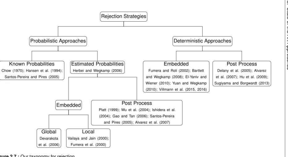
A taxonomy for rejection (Fig. 2.7): In order to provide an overview of the aforementioned approaches, we grouped some of them into a rough taxonomy. We distinguish between probabilistic and deterministic approaches. The proba-bilistic rejection approaches are based on known probabilities or estimated ones. To obtain estimated probabilities one can simply use a probabilistic classifier which provides the probability internally or one can estimate the probabilities in a post-processing step independently of the used classifier. For deterministic approaches, we distinguish between embedded rejection, which is integrated in the classifier itself and optimised during training and approaches which work as a post-processing step. The latter approaches rely also on the classifier but parameters of the reject option are not optimised while training the classifier itself. In our taxonomy only the approaches of Vailaya and Jain (2000) and Fumera et al. (2000) provide local rejection.
2.3. State of the Ar t Approaches 19 Rejection Strategies Probabilistic Approaches Known Probabilities Chow (1970); Hansen et al. (1994);
Santos-Pereira and Pires (2005)
Estimated Probabilities Herbei and Wegkamp (2006)
Embedded
Global Devarakota et al. (2006)
Local Vailaya and Jain (2000);
Fumera et al. (2000)
Post Process
Platt (1999); Wu et al. (2004); Ishidera et al. (2004); Gao and Tan (2006); Santos-Pereira
and Pires (2005); Alvarez et al. (2007)
Deterministic Approaches
Embedded Fumera and Roli (2002); Bartlett and Wegkamp (2008); El-Yaniv and Wiener (2010); Yuan and Wegkamp (2010); Villmann et al. (2015, 2016)
Post Process Delany et al. (2005); Alvarez et al. (2007); Hu et al. (2009); Sugiyama and Borgwardt (2013)
2.4. Conclusion
Summing up the state of the art leads to the following findings: In settings with known class probabilities the problem of finding the right certainty measure and the optimal global threshold is solved by Chow (1970). Many approaches estimate the class probabilities in settings where they are unavailable. Those estimations are defective to varying degrees. The main shortcoming is, that it is difficult to determine the precision of the estimated class probabilities. It turns out that local thresholds are beneficial in scenarios with defective estimations (Fumera et al., 2000). The other large group of approaches operates with deterministic certainty measures, e. g., distance-based ones. There are well studied measures available, e. g., for SVM, but there are only a few simple approaches suited for prototype-based classifiers. Often it is difficult to set an appropriate threshold for rejection since the deterministic measures, e. g., as the distance to the decision border, may not be normalised. It is even more complicated if local thresholds have to be chosen. The challenge is to determine the best possible thresholds in order to optimise the error reject trade-off.
In the next chapter, we introduce the prototype-based classifiers first, which we use later on. Afterwards, we report our research results on rejection strategies.
3. Prototype-based Classification
Chapter overview In this chapter we first motivate why we focus on prototype-based clas-sifiers. A main advantage of those classifiers is their sparsity and that they allow a meaningful interpretation. Second we describe the used classifiers which belong to the popular family of LVQ approaches and we give a brief overview of their development.
A prototype-based classifier stores prototypes for different classes. Hence such a classifier consists of a setW ofξ prototypeswj ∈RM where every prototype
wj has a class labelcj ∈ {1, . . . , Z}. A data pointx∈RM gets the same labelcl
as its closest prototype (nearest neighbour, NN)wlwith
l= arg min
j=1,...,ξ d(wj,x) (3.1)
whered(·)is a dissimilarity measure; e. g., the Euclidean distance. The closest prototype wl is called the best matching unit. By means of the rule (3.1), a
prototype-based classifier partitions the data intoVoronoi cellsorreceptive fields Vj ={x|d(wj,x)≤d(wk,x),∀k6=j}, j= 1, . . . , ξ .
The classification in a Voronoi cellVj is constant and defined by the representing
prototypewj.
A very basic approach is the nearest neighbour classifier (NNC) which uses the training data points as prototypes. The benefits of such a prototype-based classifier are:
• Prototypeswj are elements of the same space as the data (for NNC they
equal the data points) which make them interpretable and understandable. • The classification scheme is simple and understandable.
But there are disadvantages as well since the number of prototypes in a NNC equals the number of training data points, hence the model is very complex. Koho-nen (1989) proposed learning vector quantisation (LVQ) which aims at a sparser prototype-based model (Biehl et al., 2009). There the number of prototypes is predefined and the LVQ relies on the Hebbian learning paradigm (Kohonen, 1989). Although LVQ is a heuristic only, it achieves good results (Biehl et al., 2007). Due to its simple strategy and its low computational effort together with good performance,
LVQ is quite popular. In order to overcome instabilities and to achieve convergence guarantees, Sato and Yamada (1995) introduced the generalised LVQ (GLVQ) which is based on a suitable cost function. A probabilistic counterpart is the robust soft LVQ (RSLVQ) (Seo and Obermayer, 2003). Since the prototype models often focus on classification, the prototypes are discriminative. This means that they may not represent data in a generative way. Hammer et al. (2014) propose an approach enforcing generative prototypes. Due to the representation of models in terms of prototypes, LVQ schemes are suited for online scenarios (Denecke et al., 2009) or lifelong learning (Kirstein et al., 2012) as we will discuss in chapter 6.
The used dissimilarity measure of the prototype-based classifiers is a key aspect and the use of more general dissimilarity measures like e. g., divergences or functional metrics (Villmann and Haase, 2011) is easily possible. Hence a suitable dissimilarity measure for the data can be chosen, or the dissimilarity measure can be learned in addition to the prototypes because prototype-based classifiers provide a particularly efficient framework for integrating the powerful concept of metric learning (Bellet and Habrard, 2015; Bellet et al., 2013; Biehl et al., 2013b). For instance they offer efficient metric parametrisation strategies by their decomposition of the input space into Voronoi cells (see Schneider et al., 2009a,b). Recent LVQ schemes rely on a cost function and allow an extension to a global adaptive matrix: generalised matrix LVQ (GMLVQ) (Schneider et al., 2009a) and its local version (LGMLVQ) (Schneider et al., 2009a) with local adaptive matrices.
Prototype locations are usually learned on a given offline data setX withN data points(xi, yi)∈RM× {1, . . . , Z}ofZdifferent classes. The aim is to find
pro-totypes such that the induced classification of the data is as accurate as possible. A quality criterion is theaccuracy which is the percentage of correctly classified data points of the given data. For the cost function based LVQ approaches there are guarantees on the generalisation performance and learning convergence of the related classifier (Biehl et al., 2007; Schneider et al., 2009a). The family of LVQ approaches has gained much attention recently in the biomedical domain (Arlt et al., 2011; Biehl et al., 2012) and in the context of big data and interpretable models due to its flexibility and intuitive classification scheme (see e. g., Kirstein et al., 2008, 2009, 2012; Bunte et al., 2012; Giotis et al., 2013; Biehl et al., 2013a, 2015; Nova and Est ´evez, 2014; Zhu et al., 2014; de Vries et al., 2015).
NNC LVQ GLVQ GMLVQ LGMLVQ RSLVQ complex heuristic sparse heuristic cost function probabilistic deterministic static, global metric
adaptive
global metric adaptivelocal metrics
3.1. Generalised Learning Vector Quantisation 23
The sketch (Fig. 3.1) contains the relations between GLVQ, GMLVQ, LGMLVQ, and the RSLVQ which we mainly use and which we describe below.
Remark:Note that we refer todas metric, although it may not be a metric in the mathematical sense. For instance, often the squared Euclidean distance is used which is not a metric in the mathematical sense since the triangular inequality does not hold for every given set of data points.
3.1. Generalised LVQ – GLVQ
A robust LVQ approach is the GLVQ (Sato and Yamada, 1995) based on a differ-entiable cost function approximating the classification error (3.2). It minimises:
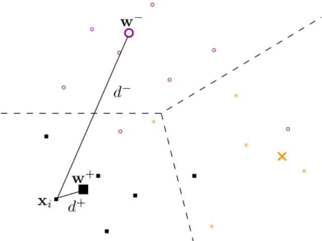
EGLVQ(X) = X 1≤i≤N Φ(µ(xi)) with µ(xi) = d+(x i)−d−(xi) d+(x i) +d−(xi) . (3.2)
The valued+(xi) = d(xi,w+)andd−(xi) = d(xi,w−)denotes the dissimilarity
between a data point xi and the closest prototype w+ belonging to the same
class and the dissimilarity of the closest prototypew−of any different class (see Fig. 3.2). The functionΦ(·)is a monotonic increasing function, e. g., the identity or the sigmoid function. The summands of (3.2) are negative if and only if the classification of the corresponding point is correct, hence the costs correlate to the overall error. In this way it optimises the so-called hypothesis margin of the classifier (Schneider et al., 2009a). Note that the LVQ cost function (3.2) approximates the loss (2.1), since it aims at minimising the empirical classification error as explained. MinimisingEGLVQ(3.2) is done by a stochastic gradient descent
d−
d+
w+
w−
xi
Figure 3.2.:Scheme of a three class setting (different colours, symbols). Bigger symbols are prototypes. For one data pointxithe quantitiesw+,w−, d+andd− are displayed.
with respect to the prototypesw+andw−, leading to the update
w±:=w±−ε·∂EGLVQ
∂w± (3.3)
with a learning rate ε > 0. Using the squared Euclidean distance d(x,w) =
kx−wk2, the derivation in the update rule (3.3) becomes ∂EGLVQ ∂w± = ∂Φ ∂µ · ∂µ ∂d± · ∂d± ∂w± ∂µ ∂d± = ±2d∓ (d++d−)2 ∂d± ∂w± =−2(x−w ±)
Hence the GLVQ’s learning rule can be specified as:
w±:=w±±ε·∂Φ ∂µ ·
4d∓
(d++d−)2 ·(x−w ±).
One limitation of the GLVQ is the chosen dissimilarity measure. Often it is difficult to chose a well suited measure since one does not know which aspects of the data are relevant for classification a priori. More advanced models, e. g., GMLVQ (next section) and LGMLVQ (sec. 3.3), learn the prototypes and the metric parameters. These methods limit the general structure of the used dissimilarity measure but the related parameters are learned in order to improve the overall performance. Hence the learned measure stresses useful aspects of the data for classification.
3.2. Generalised Matrix LVQ – GMLVQ
The GMLVQ (Schneider et al., 2009a) is established on a cost functionEGMLVQ which is the same as (3.2) but it replaces the dissimilarity measure with
dΛ(w,x) = (x−w)TΛ(x−w), (3.4) a general quadratic form. The matrixΛ = ΩTΩis positive semi definite and hence
dΛ(w,x) = [Ω(x−w)]2. Since every positive symmetricΛhas a symmetric root
Ω with Λ = Ω2, we will rely thereon in the following. The GMLVQ performs a stochastic gradient descent onEGMLVQwith respect to the prototypes and with respect to the metric parameters. A similar metric learning concept exists fork-NN and nearest class mean classifiers (Bellet et al., 2013; Mensink et al., 2013) which are related to LVQ approaches.
3.2. Generalised Matrix Learning Vector Quantisation 25
leads to a replacement of the used dissimilarity measure and its derivative ∂d±Λ ∂w± =−2ΩΩ(x−w ±) = −2Λ(x−w±) and hence ∂EGMLVQ ∂w± = ∂Φ ∂µ · ∂µ ∂d±Λ · ∂d±Λ ∂w± = ∂Φ ∂µ · ±2d∓ (d++d−)2(−2Λ(x−w ±)). (3.5)
Therefore the prototype update is
w±:=w±±ε1·∂Φ ∂µ · 4d∓Λ (d+Λ +d−Λ)2 ·Λ(x−w ± ).
Additionally the single elementsΩ(l, k)are learned through a stochastic gradient descent (3.6) onEGMLVQwith respect to these elements.
Ω(l, k) := Ω(l, k)−ε2·
∂EGMLVQ
∂Ω(l, k) (3.6)
To obtain the update rule for the elements ofΩwe need the derivation ∂dΛ
∂Ω(l, k) = (x(l)−w(l))·[Ω(x−w)]k+ (x(k)−w(k))·[Ω(x−w)]l
since it is required in the gradient (3.7) of the cost function with respect toΩ(l, k). The parameterldenotes thel-th component of the vector.
∂EGMLVQ ∂Ω(l, k) = ∂Φ ∂µ ∂µ ∂d+Λ · ∂d+Λ ∂Ω(l, k) + ∂µ ∂d−Λ · ∂d−Λ ∂Ω(l, k) (3.7)
Putting all parts of (3.6) together, leads to
Ω(l, k) :=Ω(l, k)−ε2· ∂Φ ∂µ · 2 (d+Λ +d−Λ)2· d−Λ Ω(x−w+) k x(l)−w +(l) + Ω(x−w+) l x(k)−w +(k) −d+Λ Ω(x−w−) k x(l)−w − (l) + Ω(x−w−) l x(k)−w − (k) .
The parameter ε1 and ε2 are the learning rates of the updates. They can be chosen independently but usuallyε1> ε2 holds. In order to prevent the algorithm from degeneration, the matrixΛshould be normalised (Schneider et al., 2009a). It is possible to use any optimisation solver instead of a stochastic gradient descent
![Figure 4.1.: [C14a] Contour lines of the measures for artificial 2D data. This binary prob- prob-lem consists of data of two Gaussians (symbols: ×, ◦)](https://thumb-us.123doks.com/thumbv2/123dok_us/9959189.2488407/49.892.199.764.178.538/figure-contour-measures-artificial-binary-consists-gaussians-symbols.webp)
![Figure 4.4.: [C14a] Accuracy-reject-curves for several prototype-based classifiers trained on benchmark data sets.](https://thumb-us.123doks.com/thumbv2/123dok_us/9959189.2488407/56.892.124.711.397.1021/figure-accuracy-reject-curves-prototype-classifiers-trained-benchmark.webp)