Neural networks and genetic algorithms for hierarchical multi-label classification problems

(1)

Universidade de São Paulo

2014-10

Neural networks and genetic algorithms for

hierarchical multi-label classification problems

Joint Conference on Robotics and Intelligent Systems; Best DSc Theses / MSc Dissertations Contest

in Artificial and Computational Intelligence, 9th, 2014, São Carlos.

http://www.producao.usp.br/handle/BDPI/48633

Downloaded from: Biblioteca Digital da Produção Intelectual - BDPI, Universidade de São Paulo

Biblioteca Digital da Produção Intelectual - BDPI

(2)

Preface

This volume contains the papers presented at CTDIAC 2014: the 9th Best DSc Theses / MSc Dissertations Contest in Artificial and Computational Intelligence, held on October 17-22, 2014 in S˜ao Carlos/SP, as a satellite event of JCRIS 2014. There were 32 submissions. Each submission was reviewed by at least 2 pro-gram committee members. There were 5 DSc thesis papers and 6 MSc disser-tation papers selected to the second phase of CTDIAC.

We greatly appreciate the members of the program committee that helped us to select a set of high quality papers. We also thank the JCRIS and BRACIS committees for helping us with the CTDIAC organization.

Anne Canuto Gra¸caliz Dimuro Aline Paes Karina Valdivia

(3)

Neural Networks and Genetic Algorithms for

Hierarchical Multi-Label Classification Problems

Ricardo Cerri and Andr´e C. P. L. F. de Carvalho

Instituto de Ciências Matemáticas e de Computação - ICMC Universidade de São Paulo - Campus de São Carlos Caixa Postal 668 - 13560-970 - São Carlos-SP-Brazil

Email:{cerri,andre}@icmc.usp.br

Abstract_{—In conventional classification problems, each}

in-stance of a dataset is associated with just one among two or more classes. However, there are more complex classification problems where instances can be simultaneously classified into classes belonging to two or more paths of a hierarchy. Such a hierarchy can be structured as a tree or a directed acyclic graph. These problems are known in the machine learning literature as hierarchical multi-label classification (HMC) problems. In this Thesis, two methods for hierarchical multi-label classification are proposed and investigated. The first one associates a Multi-Layer Perceptron (MLP) to each hierarchical level, being each MLP responsible for the predictions in its associated level. The method is called HMC-LMLP. The second method induces hierarchical multi-label classification rules using a Genetic Algorithm. The method is called HMC-GA. Experiments using hierarchies struc-tured as trees showed that HMC-LMLP obtained classification performances superior to the state-of-the-art method in the literature, and superior or competitive performances when using graph-structured hierarchies. The HMC-GA method obtained competitive results with other methods of the literature in both tree and graph-structured hierarchies, being able of inducing, in many cases, smaller and in less quantity rules.

• Student level: PhD;

• Date of conclusion: 05/12/2013;

• Examining board members:

– Andr´e Carlos P. L. F. de Carvalho (ICMC/USP);

– Luiz Henrique de Campos Merschmann (UFOP);

– Roseli Aparecida Francelin Romero (ICMC/USP);

– Bianca Zadrozny (IBM Research);

– Fernando Jos´e von Zuben (FEEC/UNICAMP)

• Full Thesis on-line version: http://bit.ly/1rO2zpc;

• Derived publications: – Journal publications: – [1] - dx.doi.org/10.1016/j.jcss.2013.03.007; – [2] - dx.doi.org/10.1111/coin.12011; – Conference publications: – [3] - dx.doi.org/10.1109/CEC.2013.6557604; – [4] - dx.doi.org/10.1109/BRACIS.2013.29 – [5] - dx.doi.org/10.1145/2245276.2245325; – [6] - dx.doi.org/10.1007/978-3-642-22825-4 2; – [7] - dx.doi.org/10.1109/ISDA.2011.6121678 I. INTRODUCTION

In the majority of the classification problems described in the literature, a classifier assigns a single class to a given instance, and the problem classes assume a flat structure.

However, in a variety of real-world classification problems, classes have a hierarchical structure, where they are divided into subclasses or grouped in superclasses. In addition, in-stances can be assigned simultaneously to two or more classes that belong to the same hierarchical level. These problems are known in the machine learning (ML) literature as Hierarchical Multi-Label Classification (HMC) problems. A hierarchical class structure can be represented either as a tree or as a directed acyclic graph (DAG).

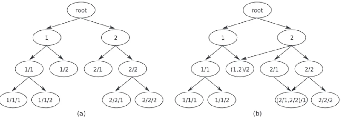
The main difference between HMC problems structured as trees and DAGs is that, in the tree structure, each node has just one parent class, whereas in the DAG structure each node may have more than one parent node. Fig. 1 depicts hierarchies structured as trees and DAGs.

Two main approaches have been used to solve HMC prob-lems: local and global. In the local approach, conventional classification algorithms, such as decision trees, are trained to produce a hierarchy of classifiers, which are later used to classify unlabeled instances following a top-down strategy [8]. In this approach, local information about the class hierarchy is used during the induction of each base classifier. According to [9], this local information can be used in different ways, depending on how the local classifiers are induced. The three main strategies for using local information are: one Local Classifier per Node (LCN), one Local Classifier per Parent Node (LCPN), and one Local Classifier per Level (LCL). The LCN strategy trains one binary classifier for each class of the hierarchy [10]. The LCPN strategy trains, for each internal class, a multi-class classifier to distinguish between its subclasses [11], and the LCL strategy trains one multi-class classifier for each hierarchical level, where each classifier is responsible for the prediction in its associated level [7].

Differently from the local approach, the global approach induces a single classifier using all classes of the hierarchy at once. After the training process, the classification of a new instance occurs in just one step [12]. As global methods induce a single classifier to consider the specificities of the classifi-cation problem, they usually do not make use of conventional classification algorithms, unless these are adapted to consider the hierarchy of classes.

The main contributions of this Thesis are as follows. First, a new HMC method termed Hierarchical Multi-Label

(5)

(HMC-Fig. 1. Hierarchies structured as: (a) trees; (b) DAGs

LMLP) is proposed, and applied to the problem of protein function prediction. The main idea is to reduce the hierarchical problem by solving a multi-label problem in each level of the class hierarchy. This is done by incrementally training a set of neural networks, one neural network per hierarchical level. Each of these neural networks is responsible for the prediction of the classes belonging to its associated hierarchical level.

Second, we propose a Genetic Algorithm (GA) to generate HMC rules. The method is called Hierarchical Multi-Label

Classification with a Genetic Algorithm (HMC-GA). It is a extended version of the method proposed in Cerri et. al. [5]. We use a new fitness function and selection operator to evolve antecedents of classification rules. The consequents of the rules are obtained using a deterministic procedure. They are represented as a class vectorv_{, where each position}

corresponds to a class, and receives a real value interpreted as the probability of an instance being classified in the class. We evolve propositional rules, which traditionally evaluates if an attribute value ak satisfies a test condition,e.g.Ak≤xi,k.

The remainder of this manuscript is organized as follows. Sections II and III present the details of the proposed meth-ods HMC-LMLP and HMC-GA. The methodology employed for the empirical analysis is discussed in Section IV. The experimental analysis is described in Section V, where the proposed methods are compared with literature methods for HMC on 20 protein function prediction datasets structured as trees and DAGs. Finally, we summarize the conclusions and discuss topics for future work in Section VI.

II. HMC-LMLP

The idea behind HMC-LMLP is to divide the learning process into a number of steps, aiming at learning a complex model through the combination of few simpler models, which are learned sequentially. By reducing the problem, each model in the sequence is forced to learn something different from the previously trained models, breaking down the complex learning process into simpler processes.

HMC-LMLP works by learning MLP networks sequentially, one for each level of the class hierarchy. Each MLP is responsible for extracting local information from the instances at each level, which we believe to be useful in the classification

of unlabeled instances. Since HMC problems are usually very complex, our hypothesis is that different patterns can be extracted from the instances in the different hierarchical levels. Note that, whereas many different classification strategies could be employed in a similar architecture, we decided for neural networks because of the simplicity in associating a class per output neuron. Therefore, obtaining a multi-label prediction for an instance is done in a straightforward fashion. In this section we present the preliminary version of the HMC-LMLP previously presented in [1], together with the new, enhanced, version. Besides, two additional baseline vari-ants are also proposed in this Thesis. For convenience, the preliminary version will be henceforth named HMC-LMLP-Labels, since it uses the classes predicted in one level as the unique input to the MLP responsible for the predictions in the next level. The new version proposed here is termed HMC-LMLP-Predicted, considering that it employs the classes predicted by an MLP in one level to complement the feature vectors of the instances used to train an MLP in the next level. The first baseline variant, called HMC-LMLP-True, employs, at each level, the true labels of the instances from the previous level to complement the feature vectors. The second baseline variant is named HMC-LMLP-NoLabels, since it uses only the original feature vectors of the instances to train the MLP at each level. For simplicity, all the networks used in this study have only one hidden layer.

A. HMC-LMLP-Labels

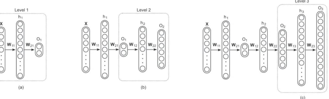
In Fig. 2, the architecture and the training process of HMC-LMLP-Labels are given. In this figure, X represents the instances assigned to classes from the level l; hl and Ol are, respectively, the hidden layer and output layer of the MLP network associated with level l. The matrices W1l and W₂_l _{represent, respectively, the weights connecting the}

input attributes and the neurons in the hidden layer, and the neurons in the hidden and output layers of the MLP associated with levell.

Initially, an MLP is associated with the first hierarchical level, having the training instances (X_{) as inputs. In order}

to allow the neural network to predict a set of labels, each output neuron is associated with one class. After the MLP

(6)

Fig. 2. Example of the HMC-LMLP-Labels architecture. (a) Training an MLP at the first level; (b) Using the output of the first MLP as input to train the MLP at the second level; (c) Using the output of the second MLP to train the MLP at the third level.

has been trained for the first hierarchical level (Fig. 2-(a)), a second MLP is associated with the next level of the hierarchy. The input for this network is now the output provided by the previously trained MLP, as shown in Fig. 2-(b). This process of incrementally training an MLP for each hierarchical level terminates when the last level of the hierarchy is reached.

When training an MLP for a specific hierarchical level, the MLPs associated with the previous levels are not re-trained, considering that their training has already taken place in the previous steps. When training an MLP for levell, the previous l−1MLP networks are used only to provide the input values for the current training process. Hence, when training an MLP for level l, its input values are obtained by feeding training instances to the MLP associated with the first level. The output values from the first MLP are then used as input to the second MLP (associated with the second level), which then provides its output values to be used as input values for the next MLP network. This process continues until the MLP associated with levellis reached. To classify unlabeled instances, these are fed into the first MLP associated with the first level. The output values of the first MLP are then used to feed the second MLP associated with the second level, and this process is repeated level by level until the last level is reached.

B. HMC-LMLP-Predicted

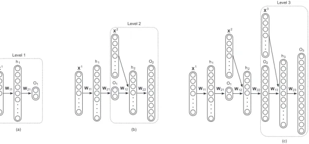
Fig. 3 illustrates the architecture of the HMC-LMLP-Predicted and its training process. In this figure,Xl_represents

the instances assigned to classes from the levell. The training process is similar to HMC-LMLP-Labels. However, each MLP from the second level onward uses the augmented feature vectors of the instances belonging to its respective associated level as inputs. The feature vectors of the instances used to train an MLP network at level l are complemented with the output from the MLP trained at levell−1.

The neural network associated with the first level is trained with all training instances (X1

), since all instances are as-signed to the classes from the first hierarchical level. At the second level, the MLP input is now the training instances that are assigned to the classes belonging to level 2 (X2

), combined with the output provided by the previously trained MLP, i.e.,

real numbers that are used to classify the instances at level 1. The advantage of using the augmented feature vector for training each MLP is the incorporation of label dependency in the learning process. A similar approach was proposed in [13]– [15], where labels were used to augment the feature space of the instances in order to enable binary classifiers to discover existing label dependency by themselves.

The training of the neural network at the third level follows the same procedure adopted for the second level (Fig. 3-(c)). This supervised incremental greedy procedure continues until the last level of the hierarchy is reached. Recall that when training an MLP network for levell, the neural network associated with levell−1 is used only to provide the inputs that will augment the feature vectors of the training instances for the MLP network associated with levell.

C. HMC-LMLP-True

The training process of HMC-LMLP-True follows the same procedure adopted in HMC-LMLP-Predicted, with the differ-ence that now the true class labels of the instances are used to complement the feature vectors, instead of the predicted class labels. Fig. 4 illustrates the architecture of the HMC-LMLP-True and the training process. In this figure, Tl are the true class labels associated to the instances at the levell. Note that now each MLP is trained separately, since an MLP associated to levell does not depend anymore on the predictions made by the MLP associated to levell−1.

D. HMC-LMLP-NoLabels

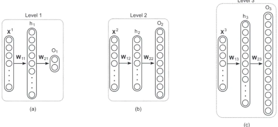
In HMC-LMLP-NoLabels, an individual MLP is trained for each hierarchical level without using the class labels (neither true nor predicted) to complement the feature vectors of the instances. Fig. 5 illustrates the HMC-LMLP-NoLabels architecture and the training process.

E. Obtaining final predictions

In the test phase of LMLP-Predicted and HMC-LMLP-True (i.e., when predicting a test instance), a top-down strategy is employed. The test instance is fed to the first MLP

(7)

Fig. 3. Example of the HMC-LMLP-Predicted architecture. (a) Training an MLP at the first level; (b) Using the output of the first MLP to augment the feature vector of the instances used to train the MLP at the second level; (c) Using the output of the second MLP to augment the feature vector of the instances used to train the MLP at the third level.

Fig. 4. Example of the HMC-LMLP-True architecture. (a) Training an MLP at the first level; (b) Using the true classes of the instances in level 1 to augment the feature vector of the instances used to train the MLP at the second level; (c) Using the true classes of the instances in level 2 to augment the feature vector of the instances used to train the MLP at the third level.

(first level), and the output from this MLP is used to com-plement the feature vector of the instance1_{. This augmented}

feature vector is then used as input to the MLP associated with the second level, whose prediction values will, once again, complement the input for the MLP at the third level. This procedure is repeated until the last MLP network, associated with the last level, is reached. As previously mentioned, in both the training and test phases of HMC-LMLP-Predicted, the augmentation of feature vectors is not incremental, i.e., the feature vector of an instance being fed into an MLP associated with levellis only complemented by the output from the MLP

1_{Recall that, in the test phase, the true labels are not available to the MLPs.}

associated with levell−1. The same is true for HMC-LMLP-True, with the difference that the true class labels are used in the training phase and the predicted classes are used in the test phase. In HMC-LMLP-NoLabels, all instances are fed into all MLPs at every level. Each MLP then gives independent predictions for the instances at each level.

To obtain the final prediction for a test instance – consider-ing all HMC-LMLP variations – thresholds are applied to the output prediction values from each of the MLPs to define the predictions for each level. If the output of a given neuronjis equal to or larger than a given threshold, the instance being classified is assigned to the class cj. The final classification from HMC-LMLP is given by a binary vectorv _{of size}_|_C_|_,

(8)

Fig. 5. Example of the HMC-LMLP-NoLabels architecture. (a) Training an MLP at the first level; (b) Training an MLP at the second level; (c) Training an MLP at the third level.

whereC is the set of all classes in the hierarchy. If the output value of neuronj is equal to or larger than a given threshold, the value 1 is assigned to positionv_{j. Otherwise, the position}

is set to 0. It is expected that different threshold values result in different predicted classes. As the activation function used in the neurons is the logistic sigmoid function, the output values range from 0 to 1. Thus, we can make use of threshold values also ranging from 0 to 1. The larger the threshold value employed, the lower the number of predicted classes will be. Conversely, the lower the threshold value employed, the larger the number of predicted classes. It is important to recall that, during the classification process, the output values that are passed from network to network are not the values obtained after the application of a threshold (0 or 1). The regular output values from the last-layer neurons, which are within [0,1], are not modified. The application of the threshold is only performed to generate the final predictions.

After HMC-LMLP has provided the final predictions, a post-processing phase is employed to correct eventual classi-fication inconsistencies, i.e., when a subclass is predicted but its superclass is not. These inconsistencies may occur because each MLP makes its predictions individually, and even though these individual MLPs make use of data from the previous levels, this does not guarantee that the superclasses of all predicted subclasses have also been predicted. This problem is intrinsic to the LCL strategy [9]. The post-processing phase guarantees that only consistent predictions are made.

We use a very simple procedure to correct inconsistencies in the predictions. Our post-processing phase simply removes from the the prediction those predicted classes that do not have predicted superclasses.

III. HMC-GA

Hierarchical Multi-Label Classification with a Genetic Al-gorithm (HMC-GA) is a global-based method for the genera-tion of HMC rules using a Genetic Algorithm (GA). The main pseudocode of the method is presented in Algorithm 1, where a sequential covering procedure is implemented to evolve antecedents of rules. In this procedure, instances covered by a rule are removed from the training set, so that new rules can

be generated with the remaining instances. The consequent of a rule is generated using a deterministic procedure considering the classes of all instances covered by the rule.

A. Individual Representation

Figure 6 illustrates the individual representation in HMC-GA. Each test of an individual is represented as a 4-tuple

{FLAG, OP, ∆1, ∆2}, where each 4-tuple is associated to

a dataset attribute A. The gene FLAG indicates if the test over an attribute is used in the rule. If the test is used,FLAG

receives the value 1, and 0 otherwise. GeneOPis the integer index of the operator used in the test. Genes∆1and∆2will

receive values that will depend on the operators used. Exactly how all values are assigned will be detailed explained in the next section.

Fig. 6. Representation of an Individual.

With the representation depicted in Figure 6, HMC-GA is able to evolve rules of the form IF Antecedent THEN

Consequent. The antecedent of a rule is thus formed by a conjunction of tests, and the consequent of a rule is formed by a set of classes, respecting the constraints of the hierar-chical taxonomy. An example of rule is given below. In this example, only active tests of the rule are shown.

IF (A1 OP ∆1) AND (∆1 OP A5 OP ∆2)

THEN

{1,1/1,1/2,1/1/1,2,2/1}

B. Population Initialization

The population in HMC-GA is initialized using a seeding procedure, where an instance is randomly selected and trans-formed into a rule. Each test has a probability pt of being used. The operator used is randomly selected depending if the attribute is numeric or categoric.

(9)

procedureHMC-GA()

Input:training setD

number of generationsG

size of population p

min number of instances covered by a ruleminCov

max number of instances covered by a rule maxCov

max number of not-covered instancesmaxN otCov

crossover ratecr

mutation ratemr

tournament sizet

number of individuals selected by elitisme

probability of using a test in a rulept

Output:set of rulesInducedRules inducedRules← ∅

while|D|> maxN otCovdo

initialP op←generateP opulation(D, p, pt) calculateF itness(initialP op, D)

currentP op←initialP op

bestRule←best rule ofcurrentP op j←G

repeat

newP op← ∅

newP op←newP op∪elitism(currentP op, e) parents←tournament(initialP op, t, e, p) of f spring←uniCrossover(parental, cr) newP op←newP op∪of f spring

newP op←mutation(newP op, mr, pt)

newP op←locOp(newP op, minCov, maxCov) currentP op←newP op

calculateF itness(currentP op, D)

bestRule←getBest(initialP op, bestRule) j←j−1

untilj >0ORruleConvergence(); inducedRules←inducedRules∪bestRule remove from Dall instances covered by bestRule

end

returninducedRules

Algorithm 1:A Genetic Algorithm to generate HMC rules.

After choosing the operator, the values to be put in the genes

∆1 and ∆2 depend on the operator chosen. For categorical

attributes, the operators can be=,6=, andin. Theinoperator verifies if a given attribute value is among a given set of values. If the operator chosen is=or6=, gene∆1 receives the index

corresponding to the categoric value of attribute in the instance being used as seed, and gene∆2receives 0 (∆2is not going to

be used in the test). If the operator isin, gene∆1receives the

index corresponding to one of the sets of values which contain the value of attribute in the instance, and gene ∆2receives 0.

As an example of this last procedure, if the attribute in the instance has the value A, and the possible attribute values in the dataset areA,B, andC, position∆1receives an index value

corresponding to one of the sets of values which contain value

A:{A, B},{A, C}, and{A, B, C}. The set of values used is randomly chosen.

If the operator chosen corresponds to an operation over a numeric attribute, the assignment of values to genes ∆1 and ∆2 is simpler, because numeric attribute values do not need

to be indexed. In the case of operator ≥, gene ∆1 receives

the attribute value in the instance, and gene ∆2 receives 0.

If the operator is ≤, gene ∆2 receives the attribute value

in the instance, and gene ∆2 receives 0. We use ∆1 and ∆2 differently depending on the operator used because we

consider ∆1 and ∆2, respectively, as the lower and upper

bounds of the attribute value. This facilitates the use of an operation testing if an attribute value is between two given values (∆1≤Ai≤∆2). In this case, the values for genes∆1

and ∆2 are randomly chosen in order to make the attribute

valueAi satisfy the test condition.

The indexation of categorical values and operators is done according to Figure 7. In the Figure, a dataset with four attributes is considered. When verifying if a rule covers an instance, appropriate operations are executed according to the type of attribute (numeric and categoric).

!" # $ !" # $ !" # $ !" # $ % % & ' & ' ( ) **( * * * **( * *+, - $, ( * ( & ' ( ) * . ( ) & ' & ' ( ) **( * * * % %

Fig. 7. Indexation of operators and categorical values.

C. Evolution

The evolutionary process starts by saving the besterules of the current population (elitism). Then,p−erules are selected to be submitted to a uniform crossover operation, in order to generate an offspring. The crossover operation exchanges entires 4-tuples between the individuals. This means that crossover points are allowed to fall only in the boundaries between two 4-tuples. In order to specialize the rules in the classification of a set of instances, the crossover operation con-siders the distances between the consequents of the rules. The consequent of a rule represents a vector of class probabilities, and each vector position value is given by Equation 1.

vr,j =

|Sr,j|

|Sr|

(1) In Equation 1,Sr,jis the set of all training instances covered by ruler, which are classified in classcj. The setSr contains all training instances covered by ruler. Thus, each position vr,j contains the proportion of instances covered by rule r, which are classified in class cj. This can be interpreted as the probability of an instance covered byrto be classified in classcj.

(10)

Our crossover operator receives as input a list of p −e rules. A rule is then removed from the list, and the weighted Euclidean distances between the consequent of this rule, and the consequents of all the other rules in the list, are calculated. The lower the Euclidean distance value between the consequents of two rules, the nearer the rules are considered to be in the search space. The two nearest rules are then removed from the list, and their antecedents are submitted to a uniform crossover to generate two child rules. The objective is to apply the crossover operator in rules that cover instances that are near in the search space,i.e., instances that are classified in a similar or equal set of classes. Equation 2 gives the calculation of the weighted Euclidean distance (WED) between the consequents of two rules. W ED(v₁_,v₂_{) =} v u u t |C| X j=1 wi×(v1,j−v2,j)2 (2)

In Equation 2,wj corresponds to the weight associated to the jth _{class in the hierarchy. Weights were associated to} each class because, in the context of hierarchical classification, similarities between classes located in levels closer to the root are more important than similarities between classes located in deeper levels [12].

The weighting scheme used in HMC-GA is the same used in [12]. After trying different schemes, the authors found out that the best one is given by Equation 3. The weight w0

associated to a class in the first level is defined as 0.75, and the weight of a classcjis recursively defined as the multiplication of w0 by the mean weight of all its ancestor classesPj.

wj=w0×

Pj X

k=1

w(pk)/Pj (3) After the generation of new rules, a mutation operator is applied to a percentage mr of them, randomly chosen. Each of the rules have a chance of 50% to suffer aFLAGmutation and a chance of 50% to suffer a restriction or generalization. In theFLAGmutation, each test in the antecedent of the rule has a probabilityptof being not used (geneFLAGexchanged from 1 to 0), or used (geneFLAGexchanged from 0 to 1). In the restriction/generalization operation, each used test in the rule is randomly restricted or generalized, having their values modified by using a randomly generated factor in [0,1]. The restriction/generalization procedure is applied in order to make the tests cover a smaller/larger number of instances.

After the mutation operation, a local operator is applied in order to try to guarantee that the rules cover a minimum and maximum number of instances. This is performed to make the rules not too specific neither too general.

After the generation of a new offspring, the fitness of all rules is calculated, and the best rule is saved. This procedure is executed until the maximum number of generations is reached, or until rule convergence, i.e. the same rule stays the same after 10 generations. After this complete evolutionary cycle is performed, the best rule found so far is saved, and its

covered instances are removed from the training data. A new population is then generated, and and new evolutionary cycle is executed. This is performed until all, or almost all, training instances are covered.

D. Fitness Calculation

HMC-GA uses the variance gain [12], [16] of a rule as its fitness. The variance gain value is higher for rules which cover a more homogeneous set of instances,i.e., rules that partition the training set in more homogeneous sets. In addition, the variance gain can directly cope with hierarchical multi-label data, considering the relationships between the classes [16]. The variance gain (VG) calculation is presented in Equation 4.

V G(r, S) =var(S)−|Sr|

|S|×var(Sr)− |S¬r|

|S| ×var(S¬r) (4)

As observed in Equation 4, the setSof all training instances is divided into two subsets: the set of instances covered by rule r, denoted Sr, and the set of instances not covered by ruler, denoted S¬r. The variance gain of a rule is obtained

considering the setS, and also involves the variance (var) of the sets Sr and S¬r. The variance of a set of instances is

defined by the sum of the mean quadratic distances between the class vector of each instance (v_{i), and the mean class label}

vector of all instances in the set (v_{). The variance of a set of}

instances S is presented in Equation 5. The distance used is the weighed Euclidean distance presented in Equation 2.

var(S) = P|S| i=1W ED(vi,v) 2 |S| (5) IV. EXPERIMENTALSET-UP

In this section, we present the HMC methods that are compared with HMC-LMLP and HMC-GA. We also de-scribe the datasets used in the experiments and the eval-uation methodology adopted for the experimental analysis. Additionally, we detail the rationale behind the parameter setting employed by HMC-LMLP, and present the parameters used in HMC-GA. The datasets used in the experiments and the source code of the proposed methods can be found in http://sites.google.com/site/cerrirc/downloads/.

Recall that not all experiments performed in the Thesis are shown in this manuscript. We selected a subset of experiments which demonstrate the good performance obtained by the pro-posed methods, and also show how promising were the results. A. HMC literature methods

We compare HMC-LMLP and HMC-GA with four literature HMC methods used for protein function prediction: PCT-based methods Clus-HMC, Clus-HSC, and Clus-SC [12]; and hmAnt-Miner [16]. These methods are briefly described next:

• Clus-HMC: global-based method that builds a single

decision tree to cope with all classes simultaneously;

• Clus-HSC: LCN-based method that applies a top-down

strategy to induce a decision tree for each hierarchical class considering the hierarchical relationships;

(11)

• Clus-SC: LCN-based method that induces one decision

tree for each hierarchical level without considering hier-archical relationships;

• hmAnt-Miner: global-based method that uses concepts from ACO to generate classification rules.

B. Datasets

Twenty freely available2_{datasets related to protein function}

prediction are used in the experiments. These datasets are related to issues like phenotype data and gene expression levels, and are structured as trees and DAGs. A description of each dataset can be found in [12].

Because there is no level definition in DAG structures (a class can be located at different levels depending on which hierarchical path is chosen from the root node to the class), we defined the depth of a class in a DAG structure as the deepest path from the class to the root node. This is necessary for the application of HMC-LMLP, since the method needs a clear separation of the classes in levels, in order to apply an MLP to each level. We chose the deepest path as the definition of depth because it guarantees that when a class is located in a levell, all its superclasses will be located in levels shallower thanl.

We performed a pre-processing step before running HMC-LMLP over these datasets, in which all nominal attribute values were transformed into numeric values using the one-attribute-per-value approach, where an attribute with k cate-gories is transformed into k binary attributes. In this study, instead of 0 and 1, the nominal attributes were assigned −1

(absence) and 1 (presence) values, which are more suited for training neural networks [17]. The attributes were then standardized (mean0and variance1). Additionally, all missing values for nominal and numeric attributes were replaced, respectively, by their mode and mean values.

C. Evaluation method

As discussed in Sections II and III, the outputs of HMC-LMLP and HMC-GA, for each class, are real values between 0 and 1. The same is true for the literature methods. Thus, in order to obtain the final predictions from all methods, a threshold value was employed. When classifying an instance, if the corresponding output value for a given class is equal to or larger than the threshold, the instance is assigned to the class. Otherwise, it is not assigned to the class.

The choice of the “optimal” threshold value is a difficult task, since low threshold values lead to many classes being assigned to each instance, resulting in high recall and low precision. On the other hand, large threshold values lead to very few instances being classified, resulting in high precision and low recall. To deal with this problem, we used precision-recall curves (PR-curves) as evaluation measure to compare the different methods. To obtain a PR-curve for a given classification method, different thresholds between [0,1] are applied to the outputs of the methods, and thus different values of precision and recall are obtained, one for each threshold

2_{http://www.cs.kuleuven.be/}∼_{dtai/clus/hmcdatasets.html}

value. Each threshold then represents a point within the PR space. The union of these points form a PR-curve, and the area under the curve is calculated. Different methods can be compared based on their areas under the PR-curves.

In order to calculate the area under the curve, the PR-points must be interpolated [18]. This interpolation guarantees that the area below the curve is not artificially increased, which would happen if the curves were constructed just connecting the points without interpolation.

In this work, we used the area under the average PR-curve (AU(P RC)). Given a threshold value, a precision-recall point (P rec, Rec) in the PR-space can be obtained through Equations (6) and (7). They correspond to the micro-average of precision and recall.

P rec= P iT Pi P iT Pi+ P iF Pi (6) Rec= P iT Pi P iT Pi+ P iF Ni (7) To verify the significance of the results, we employed the Friedman and Nemenyi statistical tests, recommended for comparisons involving many classifiers and several datasets [19]. We adopted a confidence level of 95% in the statisti-cal tests. As in [12] and [16], 2/3 of each dataset were used for inducing the classification models and 1/3 for test. We used the same data partitions suggested in [12].

D. HMC-LMLP Parameters

We investigate the performance of HMC-LMLP using the conventional Back-propagation algorithm [20]. The HMC-LMLP parameters were optimized using the Eisen validation dataset. This dataset was selected because it was one of the datasets where Clus-HMC obtained their best performances, and also because it has a relatively small number of attributes, which makes it possible to run several experiments in a reasonable amount of time. The following parameters were optimized: (i) number of neurons in each hidden layer (be-ginning with the hidden layer of the MLP network associated with the first hierarchical level, and finishing with the hidden layer of the MLP network associated with the last level), (ii) the learning rate and momentum constant used in the Back-propagation algorithm, and (iii) the range of values used to initialize the neural network’s weights. To reduce the influence of parameter selection in the MLP predictive performance, the number of hidden neurons was set as a fraction of the number of input attributes. We executed HMC-LMLP over the validation datasets using different sets of parameter values. We employed different initial weight values, number of hidden neurons, learning rates, and momentum constants. We did not use all possible sets of values due to the huge number of possibilities.

Because the datasets structured as trees and DAGs have the same attributes (only the class structure is different), and due to the high computational cost when executing HMC-LMLP using the DAG structured datasets, we performed

(12)

the parameter optimization procedure only considering the datasets structured as trees.

For the initial weights of the neural networks, we noticed that the higher their initial values are, the more likely over-fitting will occur, achieving a better performance on more frequent classes but a worse overall prediction performance. We varied the initial weights by randomly selecting them initially from [-0.1,0.1], but gradually increasing the range to [-1,1]. Regarding the number of neurons, we tested a limited number of neurons for each hidden layer, beginning with 1.0/0.9/0.8/0.7/0.6/0.5 neurons in each layer and gradu-ally decreasing these values until 0.1/0.08/0.06/0.04/0.03/0.02. These hidden neuron numbers represent the fraction of the total number of network inputs. Thus, if a neural network has 100 inputs, the value 0.6 means that it has actually 60 hidden neurons. Considering the learning rate and momentum, we started our experiments with the same values used in in the Weka tool [21], where the learning rate is set to 0.3 and the momentum to 0.2. We gradually decreased theses values and noticed that the neural networks became less liable to overfitting as these values decreased. The final parameters obtained for HMC-LMLP after the preliminary experiments are listed next.

• Number of hidden neurons per level (fraction of the total

number of network inputs):

– 0.6/0.5/0.4/0.3/0.2/0.1 for trees;

– 0.65/0.65/0.6/0.55/0.5/0.45/0.4/0.35/0.3/0.25/0.2/ 0.15/0.1 for DAGs;

• Learning rate and momentum constant used in

Back-propagation for hidden and output layers: {0.05,0.03}

and{0.03,0.01}, respectively;

• Initial weights of the neural networks: within [-0.1,0.1]; We would like to point out that we decreased the number of hidden neurons of the neural networks as the hierarchical levels become deeper. Our intention was to avoid overfitting, since the number of training instances is smaller for the networks associated with deeper hierarchical levels. For DAG-structured hierarchies, we choose 0.1 as the fraction of inputs for the MLP associated to the last level (same value obtained for trees). We then increased this value by 0.05 until the first level was reached. With this, we used values that were similar to the ones used in the tree structure.

E. HMC-GA Parameters

The parameter values used in HMC-GA are listed in Table I. These parameters were obtained based on the work of [22], and no attempts to optimize them were made. The work developed in [22] is a local-based GA to evolve rules for hierarchical, but not multi-label, problems.

The parameter pt (probability of using an attribute in initialization) has a different value according to the number of attributes in the dataset. It is given by |A| ×pt= 5, were

|A| is the number of attributes. Thus, the parameter value is set in order to activate on average 5 tests in the rule. We chose to start with small rules in order not to have an initial

TABLE I

PARAMETERS USED INHMC-GA

Parameters Values

Size of population (p) 100/500/1000

Elitism rate (e) 1%

Mutation rate (mr) 40%

Crossover rate (cr) 90%

Probability of using an attribute in initialization (pt) |A| ×pt= 5

Number of Generations (G) 100

Tournament size (t) 2

Maximum number of not-covered instances (maxN otCov) 10 Minimum number of instances covered by a rule (minCov) 10 Maximum number of instances covered by a rule (maxCov) 300

population with too many restricted rules, covering none or very few instances. We also executed HMC-GA with three different population sizes, 100, 500, and 1000 individuals.

V. RESULTS ANDDISCUSSION

In this section, we present part of the results described in the Thesis. We performed two sets of experiments. First, we show the experiments performed to compare the prediction perfor-mance of the four HMC-LMLP variations, and the baseline literature HMC algorithms. In a second set of experiments we compare HMC-GA with the literature methods.

The values depicted for HMC-LMLP and HMC-GA are the mean and standard deviation over 10 executions. For HMC-LMLP, each execution had randomly-initialized neural network weights. Given that hmAnt-Miner is a probabilistic method, we also executed it 10 times and show the mean and standard deviation over all executions. HMC, Clus-HSC, and Clus-SC are deterministic algorithms and thus need to be executed only once. We highlight in bold the best absolute values.

A. Experiments with HMC-LMLP

Table II presents the comparison among the HMC-LMLP variations and the baseline methods Clus-HMC, Clus-HSC, Clus-SC, andhmAnt-Miner.

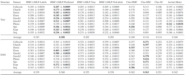
Results from Table II show that all HMC-LMLP vari-ations outperformed the two local-based methods Clus-HSC and Clus-SC by a large margin in the tree-structured datasets. Still regarding the tree-structured data, the variations Predicted, True, and HMC-LMLP-NoLabels achieved better results than the global methods Clus-HMC andhmAnt-Miner in the majority of the datasets. More-over, and as expected, the variation HMC-LMLP-Predicted obtained the best results overall among all the methods in the tree-structured datasets, and improved the results of ver-sions HMC-LMLP-True and HMC-LMLP-NoLabels, which reinforces the idea that the predictions at one level were indeed useful in the learning process of the next level.

It is interesting to see how the use of the predictions Predicted) instead of the true classes (HMC-LMLP-True) led to the improvement of the classification performance. This is an indicative that the neural networks were capable of better exploring the relationships between the classes in

(13)

TABLE II

AU₍P RC₎VALUES OBTAINED IN THE TREE AND DAG STRUCTURED DATASETS- HMC-LMLP

Structure Dataset HMC-LMLP-Labels HMC-LMLP-Predicted HMC-LMLP-True HMC-LMLP-NoLabels Clus-HMC Clus-HSC Clus-SC hmAnt-Miner

Tree Cellcycle 0.185±0.0010 0.207±0.0009 0.203±0.0013 0.205±0.0009 0.172 0.111 0.106 0.155±0.0082 Church 0.164±0.0007 0.173±0.0008 0.167±0.0016 0.169±0.0009 0.170 0.131 0.128 0.165±0.0027 Derisi 0.171±0.0010 0.183±0.0014 0.176±0.0012 0.182±0.0012 0.175 0.094 0.089 0.149±0.0078 Eisen 0.208±0.0011 0.245±0.0017 0.236±0.0013 0.240±0.0013 0.204 0.127 0.132 0.181±0.0069 Gasch1 0.196±0.0010 0.236±0.0020 0.229±0.0022 0.234±0.0016 0.205 0.106 0.104 0.173±0.0076 Gasch2 0.184±0.0007 0.211±0.0007 0.201±0.0014 0.208±0.0009 0.195 0.121 0.119 0.152±0.0006 Pheno 0.159±0.0009 0.159±0.0019 0.158±0.0011 0.159±0.0017 0.160 0.152 0.149 0.161±0.0038 Spo 0.172±0.0009 0.186±0.0016 0.180±0.0007 0.184±0.0011 0.186 0.103 0.098 0.177±0.0041 Expr 0.196±0.0030 0.243±0.0025 0.238±0.0034 0.240±0.0033 0.210 0.127 0.123 0.180±0.0066 Seq 0.195±0.0032 0.236±0.0025 0.233±0.0050 0.232±0.0040 0.211 0.091 0.095 0.186±0.0083 Average 0.183 0.208 0.202 0.205 0.189 0.116 0.114 0.168 DAG Cellcycle 0.339±0.0014 0.361±0.0010 0.352±0.0025 0.359±0.0007 0.357 0.371 0.252 0.325±0.0079 Church 0.334±0.0010 0.341±0.0009 0.336±0.0015 0.340±0.0011 0.348 0.397 0.289 0.334±0.0010 Derisi 0.334±0.0011 0.343±0.0010 0.336±0.0013 0.345±0.0006 0.355 0.349 0.218 0.321±0.0068 Eisen 0.363±0.0016 0.403±0.0017 0.393±0.0014 0.395±0.0012 0.380 0.365 0.270 0.373±0.0110 Gasch1 0.343±0.0007 0.380±0.0020 0.373±0.0029 0.378±0.0012 0.371 0.351 0.239 0.352±0.0082 Gasch2 0.340±0.0007 0.369±0.0015 0.359±0.0019 0.362±0.0012 0.365 0.378 0.267 0.334±0.0165 Pheno 0.326±0.0012 0.318±0.0020 0.315±0.0025 0.322±0.0011 0.337 0.416 0.316 0.336±0.0017 Spo 0.333±0.0015 0.342±0.0012 0.334±0.0021 0.340±0.0007 0.352 0.371 0.213 0.329±0.0078 Expr 0.336±0.0025 0.372±0.0032 0.369±0.0031 0.371±0.0014 0.368 0.351 0.249 0.343±0.0066 Seq 0.343±0.0031 0.370±0.0025 0.368±0.0034 0.368±0.0018 0.386 0.282 0.197 0.371±0.0069 Average 0.339 0.360 0.355 0.358 0.362 0.363 0.251 0.342

each level when making use of the predictions, and that these relationships were learned during the training process.

Regarding the DAG structured datasets, we can see that the overall performance of all methods were similar, except for Clus-SC, hmAnt-Miner and HMC-LMLP-Labels. Clus-HSC obtained the best results in five datasets, followed by HMC-LMLP-Predicted — that achieved the best performance in three datasets — and Clus-HMC, which obtained the best results in two datasets. If we compare the performances of the for HMC-LMLP variations, again HMC-LMLP-Predicted provided the best results for the majority of the datasets.

Afters applying the Friedman test, thep-value obtained was

1.47×10−22

, which clearly indicates that there are statistically significant differences between the methods. To identify which pairwise comparisons present statistically significant differ-ences, we performed the Nemenyi post-hoc test. According to this test, the HMC-LMLP-Predicted method outperformed HMC-LMLP-Labels, Clus-HSC, Clus-SC, and hmAnt-Miner with statistical significance, and all methods were statistically superior to Clus-SC. No statistically significant differences were detected between Predicted, HMC-LMLP-True, HMC-LMLP-NoLabels and Clus-HMC.

Although no statistically significant differences were de-tected when comparing the HMC-LMLP variations with Clus-HMC, we can observe that the results provided by HMC-LMLP-Predicted in the tree-structured datasets were often largely superior than the results obtained by Clus-HMC. Considering the DAG-structured data, we believe that HMC-LMLP-Predicted could have achieved better results if all class-relationships were employed in the training process of the method. Recall that we performed an adaptation of the DAG structures to define a unique depth for each class. The depth of a class was defined as the number of edges in the largest path from the root to the class. Therefore, not all class-relationships

were considered during classification. As an example, consider that a training instance is assigned to the paths A.C and A.B.C, and that class C is a direct subclass of both classes A and B. In this case, there are two possible depths for class C: 2 (A.C) and 3 (A.B.C). In our adaptation, class C is defined as belonging to the third level. In this case, when training a neural network for the third level, we consider class C as subclass of class B alone. So, when training a neural network to predict class C (third level), we are not using as input the information related to all its superclasses (prediction for classes A and B), but only prediction related to class B.

B. Experiments with HMC-GA

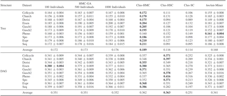
The AU(P RC) values obtained by HMC-GA are shown in Table III. The method was executed with three different numbers of individuals (rules) in the population: 100, 500 and 1000 individuals. As can be observed, in the datasets with higher number of attributes (Gasch1, Expr and Seq), the performance increased as the number of individuals was increased. This improvement is better observed in the datasets Expr and Seq.

Considering the experiments in the tree-structured datasets, the best performances were obtained by HMC-GA and Clus-HMC. In the DAG-structured datasets, the methods Clus-HMC and Clus-HSC obtained the best results, followed by HMC-GA, which outperformedhmAnt-Miner and Clus-SC.

After applying the Friedman test, thep-value obtained was

4.39×10−20

, clearly indicating that there are statistically significant differences among the methods compared. With the application of the Nemenyi post-hoc test, we verified that Clus-HMC was statistically superior to all other methods, with exception to HMC-GA using 1000 individuals. No statisti-cally significant differences were detected among the methods HMC-GA, Clus-HSC and hmAnt-Miner. Still, all methods

(14)

TABLE III

AU₍P RC₎VALUES OBTAINED IN THE TREE ANDDAGSTRUCTURED DATASETS- HMC-GA.

Structure Dataset HMC-GA Clus-HMC Clus-HSC Clus-SC hmAnt-Miner

100 Individuals 500 Individuals 1000 Individuals

Tree Cellcycle 0.164±0.004 0.163±0.007 0.167±0.008 0.172 0.111 0.106 0.155±0.008 Church 0.156±0.008 0.157±0.011 0.155±0.010 0.170 0.131 0.128 0.165±0.003 Derisi 0.168±0.005 0.167±0.004 0.168±0.004 0.175 0.094 0.089 0.149±0.008 Eisen 0.185±0.008 0.190±0.005 0.200±0.007 0.204 0.127 0.132 0.181±0.007 Gasch1 0.188±0.006 0.191±0.007 0.192±0.007 0.205 0.106 0.104 0.173±0.008 Gasch2 0.173±0.009 0.174±0.009 0.170±0.010 0.195 0.121 0.119 0.152±0.007 Pheno 0.160±0.003 0.156±0.003 0.159±0.001 0.160 0.152 0.149 0.161±0.004 Spo 0.173±0.006 0.173±0.008 0.173±0.008 0.186 0.103 0.098 0.177±0.004 Expr 0.179±0.008 0.186±0.010 0.193±0.006 0.210 0.127 0.123 0.180±0.007 Seq 0.172±0.007 0.178±0.016 0.184±0.015 0.211 0.091 0.095 0.186±0.008 Average 0.172 0.173 0.176 0.189 0.116 0.114 0.168 DAG Cellcycle 0.341±0.009 0.344±0.007 0.339±0.008 0.357 0.371 0.252 0.325±0.008 Church 0.341±0.005 0.340±0.005 0.338±0.008 0.348 0.397 0.289 0.334±0.001 Derisi 0.344±0.003 0.342±0.005 0.343±0.005 0.355 0.349 0.218 0.321±0.007 Eisen 0.380±0.004 0.375±0.009 0.377±0.011 0.380 0.365 0.270 0.373±0.011 Gasch1 0.361±0.003 0.361±0.009 0.362±0.006 0.371 0.351 0.239 0.352±0.008 Gasch2 0.351±0.007 0.354±0.008 0.352±0.004 0.365 0.378 0.267 0.334±0.016 Pheno 0.331±0.002 0.331±0.004 0.332±0.004 0.337 0.416 0.316 0.336±0.002 Spo 0.345±0.008 0.349±0.006 0.350±0.005 0.352 0.371 0.213 0.326±0.008 Expr 0.361±0.007 0.361±0.004 0.364±0.007 0.368 0.351 0.249 0.343±0.007 Seq 0.359±0.007 0.358±0.016 0.366±0.011 0.386 0.282 0.197 0.371±0.007 Average 0.351 0.351 0.352 0.362 0.363 0.251 0.341

were statistically superior to Clus-SC.

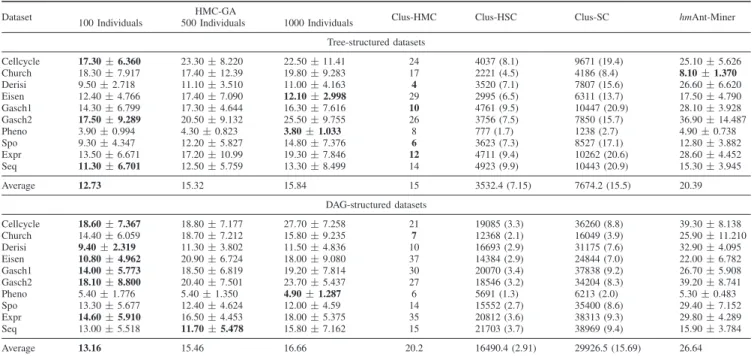
Although the prediction performance of HMC-GA was not superior to the prediction performance of the state-of-the-art method, the results can be considered promising if we consider the amount rules generated. (Table IV). HMC-GA generated fewer rules, specially for the DAG-structured hierarchies. The number of rules generated by HMC, HSC and Clus-SC is given by the number of leaves of the decision trees generated, as each path from the root node to a leaf can be considered a rule. As Clus-HSC and Clus-SC are local methods, we present the total number of rules generated by all decision trees, and also, in parentheses, the average number of rules generated by each tree. As the HMC-GA andhm Ant-Miner methods are probabilistic, the number of rules shown is the average of the number of rules obtained in each execution. The fitness function employed also has a characteristic that may have harmed the HMC-GA performance in some situations. According to Equation 4, the variance gain of a rule is maximized when the different between the variance of Sr and S¬r is minimized. However, if a very homogeneous set of training instances (instances classified in the same, or in a very similar, set or classes) is left to be covered, the fitness value can be reduced to 0. This happens when a rule which covers all instances is induced. In this case, it is a very good rule, since it covers all remaining instances belonging to a same/similar set of classes. However, its fitness value will be 0, since |S¬r|

|S| ×var(S¬r)will be 0, and the values ofvar(S)

and |Sr|

|S| ×var(Sr)will be the same.

VI. CONCLUSION

In this Thesis, we have presented two methods for HMC problems. The first one was called Hierarchical Multi-Label Classification with Local Multi-Layer Perceptron

(HMC-LMLP), which trains a Multi-Layer Perceptron (MLP) to each hierarchical level, with each MLP being responsible for the predictions in its associated level. The second one is called Hierarchical Multi-Label Classification with a Genetic Algorithm (HMC-GA), and induces HMC rules for both tree and DAG-structured hierarchies.

We performed several experiments comparing four HMC-LMLP variants and other literature methods using datasets structured as both trees and Directed Acyclic Graphs (DAGs), showing that HMC-LMLP achieved the best classification results in the tree-structured datasets, and very competitive results regarding the DAG structures. Besides, according to the experimental results, the HMC-LMLP-Predicted variant improved the classification performance when compared with HMC-LMLP-True and HMC-LMLP-NoLabels.

Regarding HMC-GA, we showed how its fitness function could have harmed the algorithm’s performance in some situations. According to the experiments, HMC-GA obtained competitive results if compared with other methods in the literature. Although HMC-GA was outperformed by the state-of-the-art Clus-HMC, the difference in their predictive perfor-mance was not statistically significant, and HMC-GA gener-ated a smaller or competitive number of rules.

As future works, we intent to use ensembles of neural networks in HMC-LMLP, and also investigate other training algorithms such as Extreme Learning Machines [23]. We also plan to improve the fitness function of HMC-GA, and extend the method to also generate rules with relational tests.

ACKNOWLEDGMENTS

The authors would like to thank the Brazilian research agencies FAPESP and CNPq, and Santander Universities. We would also like to thank Dr. Leander Schietgat and Dr. Celine

(15)

TABLE IV

NUMBER OF RULES GENERATED BYHMC-GAAND LITERATURE METHODS.

Dataset HMC-GA Clus-HMC Clus-HSC Clus-SC hmAnt-Miner

100 Individuals 500 Individuals 1000 Individuals

Tree-structured datasets Cellcycle 17.30±6.360 23.30±8.220 22.50±11.41 24 4037 (8.1) 9671 (19.4) 25.10±5.626 Church 18.30±7.917 17.40±12.39 19.80±9.283 17 2221 (4.5) 4186 (8.4) 8.10±1.370 Derisi 9.50±2.718 11.10±3.510 11.00±4.163 4 3520 (7.1) 7807 (15.6) 26.60±6.620 Eisen 12.40±4.766 17.40±7.090 12.10±2.998 29 2995 (6.5) 6311 (13.7) 17.50±4.790 Gasch1 14.30±6.799 17.30±4.644 16.30±7.616 10 4761 (9.5) 10447 (20.9) 28.10±3.928 Gasch2 17.50±9.289 20.50±9.132 25.50±9.755 26 3756 (7.5) 7850 (15.7) 36.90±14.487 Pheno 3.90±0.994 4.30±0.823 3.80±1.033 8 777 (1.7) 1238 (2.7) 4.90±0.738 Spo 9.30±4.347 12.20±5.827 14.80±7.376 6 3623 (7.3) 8527 (17.1) 12.80±3.882 Expr 13.50±6.671 17.20±10.99 19.30±7.846 12 4711 (9.4) 10262 (20.6) 28.60±4.452 Seq 11.30±6.701 12.50±5.759 13.30±8.499 14 4923 (9.9) 10443 (20.9) 15.30±3.945 Average 12.73 15.32 15.84 15 3532.4 (7.15) 7674.2 (15.5) 20.39 DAG-structured datasets Cellcycle 18.60±7.367 18.80±7.177 27.70±7.258 21 19085 (3.3) 36260 (8.8) 39.30±8.138 Church 14.40±6.059 18.70±7.212 15.80±9.235 7 12368 (2.1) 16049 (3.9) 25.90±11.210 Derisi 9.40±2.319 11.30±3.802 11.50±4.836 10 16693 (2.9) 31175 (7.6) 32.90±4.095 Eisen 10.80±4.962 20.90±6.724 18.00±9.080 37 14384 (2.9) 24844 (7.0) 22.00±6.782 Gasch1 14.00±5.773 18.50±6.819 19.20±7.814 30 20070 (3.4) 37838 (9.2) 26.70±5.908 Gasch2 18.10±8.800 20.40±7.501 23.70±5.437 27 18546 (3.2) 34204 (8.3) 39.20±8.741 Pheno 5.40±1.776 5.40±1.350 4.90±1.287 6 5691 (1.3) 6213 (2.0) 5.30±0.483 Spo 13.30±5.677 12.40±4.624 12.00±4.59 14 15552 (2.7) 35400 (8.6) 29.40±7.152 Expr 14.60±5.910 16.50±4.453 18.00±5.375 35 20812 (3.6) 38313 (9.3) 29.80±4.289 Seq 13.00±5.518 11.70±5.478 15.80±7.162 15 21703 (3.7) 38969 (9.4) 15.90±3.784 Average 13.16 15.46 16.66 20.2 16490.4 (2.91) 29926.5 (15.69) 26.64

Vens for providing support with the PCT-based methods, and Dr. Fernando Otero for providing support with the hm Ant-Miner method. Ricardo Cerri is funded by grant 2009/17401-2, S˜ao Paulo Research Foundation (FAPESP).

REFERENCES

[1] R. Cerri, R. C. Barros, and A. C. P. L. F. Carvalho, “Hierarchical multi-label classification using local neural networks,”Journal of Computer and System Sciences, vol. 80, no. 1, pp. 39–56, 2013.

[2] R. Cerri, G. L. Pappa, A. C. P. Carvalho, and A. A. Freitas, “An extensive evaluation of decision tree-based hierarchical multilabel classification methods and performance measures,” Computational Intelligence, pp. n/a–n/a, 2013, accepted for publication.

[3] R. Cerri, R. C. Barros, A. C. P. L. F. de Carvalho, and A. Freitas, “A grammatical evolution algorithm for generation of hierarchical multi-label classification rules,” inIEEE Congress onEvolutionary Computa-tion (CEC), June 2013, pp. 454–461.

[4] R. Cerri, R. C. Barros, and A. C. P. L. F. Carvalho, “Neural networks for hierarchical classification of g-protein coupled receptors,” inBrazilian Conference on Intelligent Systems (BRACIS), Oct 2013, pp. 125–130. [5] ——, “A genetic algorithm for hierarchical multi-label classification,” in

Proceedings of the 27th Annual ACM Symposium on Applied Computing, ser. SAC ’12. New York, NY, USA: ACM, 2012, pp. 250–255. [6] R. Cerri and A. C. P. L. F. Carvalho, “Hierarchical multilabel protein

function prediction using local neural networks,” inBrazilian Symposium on Bioinformatics, ser. Lecture Notes in Bioinformatics. Berlin, Heidelberg: Springer-Verlag, 2011, pp. 10–17.

[7] R. Cerri, R. Barros, and A. de Carvalho, “Hierarchical multi-label classification for protein function prediction: A local approach based on neural networks,” in Intelligent Systems Design and Applications (ISDA), nov. 2011, pp. 337 –343.

[8] E. P. Costa, A. C. Lorena, A. C. P. L. F. Carvalho, and A. A. Freitas, “Comparing several approaches for hierarchical classification of proteins with decision trees,” in Brazilian Symposium on Bioinformatics, ser. LNBI, vol. 4643. Springer-Verlag, 2007, pp. 126–137.

[9] C. Silla and A. Freitas, “A survey of hierarchical classification across different application domains,”Data Mining and Knowledge Discovery, vol. 22, pp. 31–72, 2010.

[10] G. Valentini, “True path rule hierarchical ensembles,” inInternational Workshop on Multiple Classifier Systems, 2009, pp. 232–241.

[11] S. Kiritchenko, S. Matwin, and A. F. Famili, “Hierarchical text cate-gorization as a tool of associating genes with gene ontology codes,” in

European Workshop on Data Mining and Text Mining in Bioinformatics, 2004, pp. 30–34.

[12] C. Vens, J. Struyf, L. Schietgat, S. Dˇzeroski, and H. Blockeel, “Decision trees for hierarchical multi-label classification,” Machine Learning, vol. 73, pp. 185–214, 2008.

[13] J. Read, B. Pfahringer, G. Holmes, and E. Frank, “Classifier chains for multi-label classification,” in European Conference on Machine Learning and Knowledge Discovery in Databases: Part II, ser. ECML PKDD ’09. Berlin, Heidelberg: Springer-Verlag, 2009, pp. 254–269. [14] K. Dembczynski, W. Cheng, and E. H¨ullermeier, “International

confer-ence on machine learning,” inICML, J. F¨urnkranz and T. Joachims, Eds. Omnipress, 2010, pp. 279–286.

[15] E. A. Cherman, J. Metz, and M. C. Monard, “Incorporating label depen-dency into the binary relevance framework for multi-label classification,”

Expert Systems with Applications, vol. 39, no. 2, pp. 1647–1655, 2012. [16] F. Otero, A. Freitas, and C. Johnson, “A hierarchical multi-label classi-fication ant colony algorithm for protein function prediction,”Memetic Computing, vol. 2, pp. 165–181, 2010.

[17] S. Haykin, Neural Networks: A Comprehensive Foundation, 2nd ed. Upper Saddle River, NJ, USA: Prentice Hall PTR, 1999.

[18] J. Davis and M. Goadrich, “The relationship between precision-recall and roc curves,” inInternational Conference on Machine Learning, 2006, pp. 233–240.

[19] J. Demˇsar, “Statistical comparisons of classifiers over multiple data sets,”

Journal of Machine Learning Research, vol. 7, pp. 1–30, 2006. [20] D. E. Rumelhart and J. L. McClelland,Parallel distributed processing:

explorations in the microstructure of cognition, D. E. Rumelhart and J. L. McClelland, Eds. Cambridge, MA: MIT Press, 1986, vol. 1. [21] M. Hall, E. Frank, G. Holmes, B. Pfahringer, P. Reutemann, and I. H.

Witten, “The WEKA data mining software: an update,”SIGKDD Explor. Newsl., vol. 11, no. 1, pp. 10–18, 2009.

[22] R. Carvalho, G. Brunoro, and G. Pappa, “Hcga: A genetic algorithm for hierarchical classification,” inIEEE Congress on Evolutionary Compu-tation, June 2011, pp. 933–940.

[23] G.-B. Huang, Q.-Y. Zhu, and C.-K. Siew, “Extreme learning machine: a new learning scheme of feedforward neural networks,” in IEEE International Joint Conference on Neural Networks, vol. 2, July 2004, pp. 985–990 vol.2.