PhD Dissertation
International Doctorate School in Information and Communication Technologies
DISI - University of Trento
Structural Kernels and Neural Network Models
for Question Answering Systems
Massimo Nicosia
Advisor:
Prof. Alessandro Moschitti
Universit`a degli Studi di Trento
Abstract
Tree kernels and neural networks are powerful machine learning models for extracting pat-terns from data. Tree kernels compute the similarity between two tree-structured text rep-resentations that may incorporate syntactic and semantic information. Neural networks map words into informative embeddings, and learn complex non-linear decision functions by applying a number of transformations to the input. Joining the two approaches is an exciting research direction. In this work, which is set in a Question Answering (QA) con-text, we apply the individual models to classification and ranking tasks. More importantly, we explore the intersection of tree kernels and neural networks, with the goal of developing more accurate models.
Initially, we focus on a challenging QA task, the resolution of Crossword Puzzles (CPs), and improve an automatic CP solver by tackling two problems: (i) answering crossword clues by reranking snippets from a search engine, and (ii) clue paraphrasing, which is extremely useful for finding clues with the same answers. We apply reranking models based on syntactic structures, and therefore tree kernels, to increase the accuracy and speed of the solver. In addition, we design and evaluate a composite kernel that combines a kernel over structures, and a kernel on neural network induced representations.
Going beyond the neural feature vector approach, we develop a structural kernel that exploits a deep siamese network for evaluating the similarity between words. We assess the resulting model on two classification tasks: question classification and sentiment analysis. To conclude, we study QA models that establish links between question and candidate answer passages using semantic information. First, we present our tree kernel model for answer sentence selection, which captures relations between important question words and entities in the answer. Then, we build a neural network model that can be trained to extract semantic features from text, and eventually establish links between text pairs. We show that such network is able to better model the notion of question-answer relatedness on several QA datasets, compared to the tree kernel model.
Acknowledgements
The past years in academia have been the most important of my life. During this time, I have learned countless valuable lessons that greatly contributed to what I am now. I was lucky to meet a lot of amazing people on my path. Everyone of them taught me something or inspired me to pursue my goals and ambitions. I have been also able to travel to incredible places, attend conferences, and enjoy a freedom that is not easily attainable in other situations.
I would like to thank all the people encountered during this journey. First of all, my advisor Alessandro Moschitti, who helped me navigate through the time spent in doing research; for his advices, the trust put in me, and for his precious mentorship and support. Giovanni Semeraro, who sparked my interest in machine learning and natural language processing with his course at the University of Bari. The people at the Qatar Computing Research Institute, and in particular Preslav Nakov and Lluis Marquez. I would like to thank the extraordinary researchers who hosted me at Google: Katja Filippova, Enrique Alfonseca and Aliaksei Severyn, during my first and third crucial internships at Google Zurich; Bernd Bohnet, Ryan McDonald and Michael Collins, with whom I had the pleasure of working at Google London, during my second intership. A shout-out is for my Google Zurich friends Francesco and Antonio: I cannot wait to join you in July and be your colleague again. An additional thank you goes to Aliaksei, who was not only a superb host, but also an amazing friend and collaborator on several joint papers during our overlapping time in Trento. Here, I was grateful to be part of the iKernels group and to share time and adventures with great friends, students and researchers. Thanks Antonio, Gianni, Irina, Daniele, Olga, Katya, Azad and Liah.
I would like to express my gratitude to my family for its infinite love and support: my special mum, dad, Fabio, Manu, Enzo, and my little nieces Sofia and Gaia, pure twinkles of joy. I hope to always make you proud. I also cheer my friends in Monopoli, who were always happy to see me when I was back. The last thank you is for Clelia. Without your love and caring this journey would have not been so colorful and happy.
Contents
1 Introduction 1
1.1 Motivations . . . 1
1.2 Contributions and Structure of the Thesis . . . 2
2 Support Vector Machines and Kernel Methods 7 2.1 Supervised Learning . . . 7
2.1.1 Empirical Risk Minimization . . . 8
2.1.2 Loss Function . . . 8
2.1.3 Discriminative Training . . . 8
2.2 Supervised Learning Problems in NLP . . . 9
2.2.1 Classification . . . 9
2.2.2 Reranking . . . 10
2.3 Support Vector Machines . . . 12
2.3.1 Primal Formulation . . . 12
2.3.2 Dual Formulation . . . 13
2.3.3 The Kernel Trick . . . 14
2.4 Structural Kernels . . . 15
2.4.1 String Kernel . . . 16
2.4.2 Convolution Tree Kernels . . . 16
2.5 Summary . . . 19
3 Neural Networks for Sentence Modeling 21 3.1 Neural Networks . . . 21
3.1.1 Activation Functions . . . 23
3.1.2 Training the Network . . . 24
3.1.3 Loss Functions . . . 24
3.1.4 Backpropagation . . . 25
3.2 Word Representations and the Sentence Matrix . . . 25
3.2.1 Word Representations from Language Models . . . 26
3.2.2 Word Representations from Co-occurence Prediction . . . 26
3.2.3 Word Embedding and Sentence Matrices . . . 26
3.3 Neural Bag-Of-Words . . . 27
3.4 Recurrent Networks . . . 28
3.5 Convolutional Neural Networks . . . 30
3.5.1 Convolution Feature Maps . . . 30
3.6 Siamese Networks . . . 31
3.7 Sentence Matching . . . 31
3.8 Hybrid Siamese Network . . . 34
3.8.1 Overview . . . 34
3.8.2 Sentence Matching with Hybrid Siamese Networks . . . 35
3.8.3 Experiments . . . 37
3.8.4 Conclusion . . . 40
3.9 Summary . . . 41
4 Structural Representations for Reranking Text Pairs 43 4.1 Overview . . . 44
4.2 Related Work . . . 45
4.3 WebCrow . . . 46
4.3.1 WebSearch Module (WSM) . . . 47
4.3.2 Database Module (CWDB) . . . 47
4.4 Learning to Rank with Kernels . . . 47
4.4.1 Kernel Framework . . . 48
4.4.2 Relational Shallow Tree Representation . . . 48
4.4.3 Tree Kernels for Candidate Reranking . . . 49
4.4.4 Snippet Reranking . . . 49
4.4.5 Similar Clue Reranking . . . 50
4.4.6 Similarity Feature Vector . . . 51
4.5 Experiments on Snippet Reranking and Clue Retrieval . . . 52
4.5.1 Experimental Setup . . . 52
4.5.2 Snippet Reranking . . . 53
4.5.3 Similar clue retrieval . . . 54
4.5.4 Impact on WebCrow . . . 55
4.6 Learning to Rank Aggregated Answers . . . 56
4.6.1 Aggregation Models for Answer Reranking . . . 57
4.7 Experiments on Answer Aggregation . . . 58
4.7.1 Database of Previously Solved CPs (CPDB) . . . 58
4.7.2 Experimental Setup . . . 58
4.7.3 Ranking Results . . . 59
4.8 Conclusion . . . 60
5 Kernels Based on Neural Models 61 5.1 Tree and Deep Networks-based Kernels for Reranking . . . 61
5.1.1 Clue Retrieval and Reranking . . . 62
5.1.2 Reranking with Kernels . . . 62
5.1.3 Distributional Models for Clue Reranking . . . 62
5.1.4 Experimental Settings . . . 64
5.1.5 Results . . . 65
5.1.6 Summary and Future Work . . . 66
5.2 Semantic Tree Kernels using Networks-based Similarities . . . 67
5.2.1 Related Work . . . 68
5.2.2 Tree Kernels-based Lexical Similarity . . . 69
5.2.3 Context Word Embeddings for SPTK . . . 71
5.2.4 Recurrent Networks for Encoding Text . . . 71
5.2.5 Contextual Word Similarity Network . . . 71
5.2.6 Experimental Settings . . . 73
5.2.7 Context Embedding Results . . . 76
5.2.8 Results of our Bidirectional GRU for Word Similarity . . . 78
5.2.9 Sentiment Classification Results . . . 78
5.2.10 Wins of the BiGRU model . . . 79
5.2.11 Summary . . . 80
5.3 Conclusion . . . 80
6 Semantic Linking in Convolutional Models 81 6.1 Question Analysis . . . 81
6.1.1 Question Classification . . . 82
6.1.2 Question Focus Identification . . . 82
6.2 Semantic Linking in Convolution Tree Kernels . . . 82
6.2.1 Learning to Rank with Kernels . . . 83
6.2.2 Relational Structural Models of Q/A Pairs . . . 83
6.2.3 Feature Vector Representation . . . 85
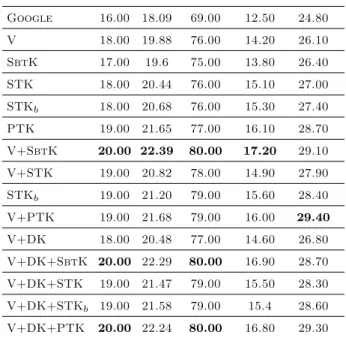
6.3 Comparison with State-Of-The-Art Systems . . . 87
6.3.1 Setup . . . 87
6.3.2 Evaluation Measures . . . 87
6.3.3 Results . . . 88
6.3.4 Summary . . . 88
6.4 Semantic Linking in CNNs . . . 89
6.4.1 Overview . . . 89
6.4.2 Related Work . . . 91
6.4.3 LTR Answer Passages with CNNs . . . 92
6.4.4 Experimental Settings . . . 98
6.4.5 Question Classification . . . 99
6.4.6 Question Focus Identification . . . 100
6.4.7 TrecQA . . . 101
6.4.8 WikiQA . . . 103
6.4.9 YahooQA . . . 105
6.4.10 Discussion and Error Analysis . . . 107
6.4.11 Summary and Future Work . . . 108
7 Conclusion and Future Work 109
Bibliography 111
List of Tables
3.1 Common activation functions. . . 24 3.2 Test accuracies of our models for the paraphrase identification task (Quora),
trained with the different losses. . . 38 3.3 Test accuracies of our models for the textual entailment task (SNLI),
trained with the different losses. . . 38 3.4 Comparison between the accuracies of the models in Wang et al. [2017] and
our models (trained with the joint loss), for the paraphrase identification task (Quora). . . 40
4.1 Clue ranking for the query: Kind of connection for traveling computer users (wifi). . . 50 4.2 Snippet reranking. . . 53 4.3 Reranking of similar clues. . . 54 4.4 Performance on the word list candidates averaged over the clues of 10 entire
CPs. . . 55 4.5 Performance given in terms of correct words and letters averaged on the 10
CPs. . . 56 4.6 Similar Clue Reranking. . . 59 4.7 Answer reranking. . . 59 5.1 SVM models and DNN trained on 120k (small dataset) and 2 millions (large
dataset) examples. Feature vectors are used with all models except when indicated by −FV. . . 65 5.2 QC accuracy (%) of SVM [Silva et al., 2010], DCNN [Kalchbrenner et al.,
2014], CNNns [Kim, 2014], DepCNN, [Ma et al., 2015] and SPTK [Croce
et al., 2011] models. . . 69 5.3 QC test set accuracies (%) of NSPTK, given embeddings with window size
equal to 5, and dimensionality ranging from 50 to 1,000. . . 76
5.4 QC cross-validation accuracies (%) of NSPTK with the embeddings of
spec-ified dimensions. . . 77
5.5 QC accuracies for the word embeddings (CBOW vectors with 500 dimen-sions, trained using hierarchical softmax) and paragraph2vec. . . 77
5.6 QC accuracies for NSPTK, using the word-in-context vector produced by the stacked BiGRU encoder trained with the Siamese Network. Word vec-tors are trained with CBOW (hs) and have 500 dimensions. . . 78
5.7 SC results for NSPTK with word embeddings and the word-in-context em-beddings. Runs of selected systems are also reported. . . 79
5.8 Sample of sentences where NSPTK with word vectors fails, and the BiGRU model produces correct classifications. . . 79
6.1 Accuracy (%) of focus classifiers. . . 84
6.2 Accuracy (%) of question classifiers. . . 85
6.3 Mapping between question classes and named entity types. . . 86
6.4 Answer sentence reranking on TrecQA.† indicates that the improvement delivered by adding F linking to CH+Vadv model is significant (p<0.05).. . . 89
6.5 Mapping between question categories and OntoNotes entity types. . . 98
6.6 Comparison between a CNN model with static embeddings [Kim, 2014] and our model. The difference in performance can be quantified in 8 mis-classified instances. . . 100
6.7 Comparison of the cross-validation accuracies between PTK, a tree kernel based classifier [Severyn and Moschitti, 2013], and our CNN model. . . 100
6.8 MAP and MRR (%) on the TrecQA Clean dataset. . . 102
6.9 MAP and MRR (%) on the WikiQA dataset. . . 103
6.10 P@1 and MRR (%) on YahooQA. The first group of results is reported in Tay et al. [2017]. The second group of results is reported in Wan et al. [2016]. The third and final group of results is related to our convolutional models: basic, with word overlap, and with word and semantic overlap. . . 104 6.11 A question along with different answer sentence candidates from the
Wik-iQA dataset. The first column report the gold standard annotation, i.e., Relevant (R) or Irrelevant (I) labels whereas the last three columns report the CNN score using word and semantic links, only word links and no link. 106
List of Figures
3.1 The Multilayer Perceptron (MLP), a feedforward network with two hidden
layers. . . 22
3.2 The CBOW and Skip-gram models [Mikolov et al., 2013b]. . . 27
3.3 A Siamese network with CNN encoders [Chopra et al., 2005]. . . 32
3.4 The Hybrid Siamese Network. . . 36
4.1 The architecture of WebCrow [Barlacchi et al., 2014b]. . . 46
4.2 Shallow syntactic trees of clue (top) and snippet (bottom) and their rela-tional links. . . 48
4.3 Two similar clues leading to the same answer. . . 50
5.1 Distributional model for computing similarity between clues [Severyn et al., 2015]. . . 63
5.2 The Lexical Centered Tree (LCT) of the lemmatized sentence: “What is an annotated bibliography?”. . . 70
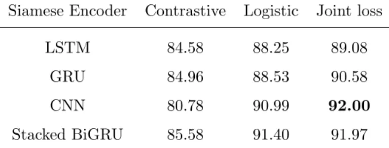
5.3 The architecture of the siamese network. The network computessim(f(s1,3), f(s2,2)). The word embeddings of each sentence are consumed by a stack of 3 Bidi-rectional GRUs. The two branches of the network share the parameter weights. . . 74
6.1 Shallow tree structure CH with a typed relation tag REL-FOCUS-HUM to link a question focus wordname with the named entities of typePerson corresponding to the question category (HUM). . . 86
6.2 The S&M CNN model. Diagram from Severyn and Moschitti [2016]. . . 95
6.3 Answer sentence reranking network with word and semantic overlap vectors. 97 6.4 Percentage of training question/answer pairs (y-axis) where the question is classified with the corresponding question type (x-axis) by our question classifier. . . 107
List of Acronyms
API Application Programming Interface
BOW Bag Of Words
BiMPM Bilateral Multi Perspective Matching CBOW Continuous Bag Of Words
CNN Convolutional Neural Network CP Crossword Puzzle
CPDB Crossword Puzzle Database CWDB Cross Word Database
DB Database
DLM Deep Learning Model DNN Deep Neural Network FC Focus Classifier
GRU Gated Recurrent Unit IR Information Retrieval LCT Lexical Centered Tree LD Large Dataset
LDC Lexical Decomposition LGR Logistic Regression
LSTM Long Short Term Memory LTR Learning To Rank
MAP Mean Average Precision MRR Mean Reciprocal Rank NBOW Neural Bag Of Words NE Named Entity
NER Named Entity Recognition NLP Natural Language Processing
NSPTK Neural Smoothed Partial Tree Kernel POS Part Of Speech
PTK Partial Tree Kernel QA Question Answering QC Question Classification QF Question Focus
ReLU Rectified Linear Unit RNN Recurrent Neural Network
SC Sentiment Classification SCR Similar Clue Retrieval SD Small Dataset
SE Search Engine
SPTK Smoothed Partial Tree Kernel STK Syntactic Tree Kernel
STS Semantic Textual Similarity SVM Support Vector Machine TK Tree Kernel
TS Text Snippet
UIMA Unstructured Information Management Applications cQA Community Question Answering
q/a question/answer
Chapter 1
Introduction
In this section, we present the motivations behind this work, and describe our contribu-tions chapter by chapter, including references to the corresponding publicacontribu-tions.
1.1
Motivations
Many Natural Language Processing (NLP) tasks require the understanding of relations between multiple pieces of text. For example in automated Question Answering (QA), the question is put in relation with text fragments that are retrieved from a document collection, usually by a search engine. These fragments may or may not contain the answer to the question, and a machine learning system must determine to what extent this fact is true for a given passage, in order to provide relevant information to a user.
This and other complex tasks often require the manual definition of rules which capture syntactic and semantic patterns useful to characterize the relations between pieces of text. One way to do this is to compute similarities between text fragments, but that does not address the specificity of the given NLP task. Usually, the most accurate methods include the manual design of specialized rules that are triggered when patterns in the pieces of text are found. These rules exploit the output of NLP processors such as parsers. The number and the complexity of rules required for making accurate decisions can be very high, and this leads to systems that are hard to mantain and difficult to develop.
While previous research showed that such systems are effective, they suffer of major drawbacks: (i) being based on heuristics they do not provide a definitive methodology, since natural language is too complex to be characterized by a finite set of rules; and (ii) given the latter claim, new domains and languages require the definition of specific rules, which causes a large effort in engineering NLP systems.
An alternative to manual rule definition is the use of machine learning, which often shifts the problem to the easier task of feature engineering. This is very convenient for
2 Introduction
simple text categorization problems, such as document topic classification, where simple bag-of-words (BOW) models have been shown to be very effective, e.g., Yang [1999]; Joachims [1998]. Treating words as atomic units has evident limitations. Although this approach is simple, robust and scalable, it does not encode any notion of similarity and it ignores the context in which words appear, unless n-grams are considered. Even so, this only allow the presence of co-occurrent words to be signalled.
When the learning task is more complex, as in QA, features have to encode the combi-nation of syntactic and semantic properties, which basically assume the shape of high-level rules: these are essential to achieve state-of-the-art accuracy. For example, the famous IBM Watson system Ferrucci et al. [2010] also includes a learning to rank algorithm fed with hundreds of features. Some of the latter are extracted with articulated rules, which are very similar to those that can be found in typical manually engineered QA systems.
In order to avoid recurrent engineering efforts, we develop methods focused on au-tomatic feature engineering. In this work, we seek to explore and eventually combine two state-of-the-art approaches for automatic feature engineering: deep neural networks (DNNs) and structural kernels. The former learn to represent text by generating in-formative embeddings and by combining them. The latter capture similarities between structural representations of text which include syntactic and semantic information. Since the latest results in kernel technology enable the use of semantic similarities between the dimensions of the substructure space, and thus the possibility to integrate the output of DNNs, there are exciting potential research directions in merging the two approaches. In particular, we aim at using DNNs for learning the representations of words and the substructures that they form when combined with syntactic and semantic elements. We want to construct pipelines that take advantage of the automatic feature engineering capabilities of these methods and make them usable in a unified framework.
1.2
Contributions and Structure of the Thesis
In Chapter 2, we introduce the reader to the general concepts which recur in this thesis. Support Vector Machines (SVMs) and kernel methods are at the core of the supervised learning setup of most of our contributions. We also give a formal definition of the struc-tural kernels that we use to tackle the two typologies of NLP tasks in the thesis: reranking and text classification.
In Chapter 3, we give a brief overview of distributional representations for words and neural network architectures. Among those, we describe the siamese network architec-ture, which give us the opportunity to present the first contribution of this thesis.
Contributions and Structure of the Thesis 3
Contribution 1 (Chapter 3). A Hybrid Siamese Network with a multi-loss setup for detecting question similarity and entailment/contradiction relations.
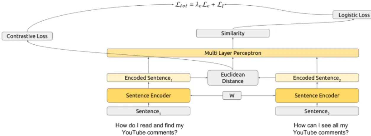
We describe a siamese network architecture that uses a multi-loss setup, which improves over single-loss setups [Nicosia and Moschitti, 2017a]. This is achieved with less com-putations than more sophisticated methods, and obtaining strong performances. A loss on the euclidean distance between two encoded sentences acts as a regularizer on their representations, while an additional logistic loss models their interaction.
In Chapter 4, we show that structural representations and kernels are powerful meth-ods for paraphrasing and for answer candidate selection. We apply our models to the automatic resolution of Crossword Puzzles (CPs), which can be seen as an untraditional QA instantiation. We tackle two tasks with the goal of improving the automatic resolu-tion of this challenging linguistic game: the retrieval of similar clues, and the selecresolu-tion of text snippets containing the answer to a target clue. The first task is an instantiation of the question-question similarity problem, while the second is the classical candidate answer passage selection task. Here we detail the contributions from this chapter.
Contribution 2 (Chapter 4). State-of-the-art retrieval of similar clues and answer passage reranking, resulting in an increase of accuracy and speed for the WebCrow cross-word solver, which has been extended with the inclusion of our modules.
State-of-the-art automatic CPs solvers typically contain modules that given a clue (i) search a database of previously solved puzzles for similar clues which may have the same answer; (ii) retrieve search engine snippets using the clue as query, and determine which of the former may contain the answer. We use tree kernels on structures to rerank clue-clue and clue-snippet pairs, and we feed our reranked list to the CP solver. Our compo-nents greatly increase the quality of the solver inputs, which results in more accurate CP completion, and shorter execution time [Barlacchi et al., 2014a,b; Nicosia et al., 2015; Barlacchi et al., 2015].
Contribution 3 (Chapter 4). UIMA pipeline for the NLP analysis of documents and for the reranking of query-passage pairs.
The system developed for the reranking of text pairs is based on the UIMA framework, which is also the foundation upon which the famous IBM Watson system is built. Our
4 Introduction
software artifact [Tymoshenko et al., 2017] has pushed the collaboration in our group and within other groups, resulting in several publications and strong results in semantic evaluation (SemEval) competitions.
In Chapter 5, we conduct our experiments on the interaction between tree kernel and neural network models. We first focus on neural networks as feature extractors, and study the inclusion of such features in our kernel-based classifiers. After this initial ex-ploration, we move into incorporating word representations learned with neural networks directly in the computation of the kernel similarity.
Contribution 4 (Chapter 5). State-of-the-art retrieval of similar clues for the res-olution of CPs, and exploration of the effectiveness of neural network features combined with structural kernels.
We again tackle the task of retrieving and reranking similar crossword clues, studying tree kernels and deep neural models [Severyn et al., 2015]. This time, we train a neural network on a large dataset of clue pairs. Our network is computationally efficient and can take advantage of the large amount of data, showing a large improvement over the tree kernel approach when the latter uses small training data. In contrast, when data is scarce, tree kernels outperform the network. We also study the interaction of tree kernels and network features, by extracting the activations of the latter, and feeding them into a multiple SVM kernel classifier. Since we use structural representations of text, we effec-tively combine a kernel on trees and a kernel over the network features.
Contribution 5 (Chapter 5). Novel semantic kernel that computes the kernel sim-ilarity considering neural representations of words, which are optimized for the end task and also include context information.
We combine tree kernels and neural networks by modeling context word similarity in semantic tree kernels [Nicosia and Moschitti, 2017b]. This way, the latter can operate subtree matching by applying neural-based similarity on tree lexical nodes. We study how to learn representations for the words in context such that tree kernels can exploit more focused information. We found that neural embeddings produced by current methods do not provide a suitable contextual similarity. For this reason, we define a new approach based on a siamese network, which produces word representations while learning a binary text similarity. We define the latter considering examples in the same category as similar. The experiments on question and sentiment classification show that our semantic tree
Contributions and Structure of the Thesis 5
kernel highly improves previous results.
In Chapter 6, we automatically learn complex patterns between pieces of text, such as re-lational semantic structures that occurr in questions and their answer passages. We focus on convolutional models: convolution tree kernels and convolutional neural networks. We provide the tree kernel with tree representations built from the syntactic trees of ques-tions and passages, after connecting them with relational tags determined by automatic classifiers, such as question and focus classifiers, and Named Entity Recognizers (NERs). This way, effective structural relational patterns are implicitly encoded in the represen-tation, and can be automatically utilized by powerful machine learning models such as kernel methods. In addition to this, we propose a fully convolutional neural network sys-tem that encodes the same information of the structural model, but has two important advantages: it is much faster to train and reaches superior performances.
Contribution 6 (Chapter 6). Semantic links between question and answer passages increase the accuracy of convolutional models. A fully convolutional neural network model shows improved accuracy and shorter training time than its counterpart based on kernels on structural representations.
We focus on the task of answer sentence selection and propose an SVM model based on a kernel over structural representations. We encode questions and answers using trees containing words, syntactic information, and semantic information in the form of tags. The tags are used to mark the question focus word, and the named entities in the answer. Additionally, tags are typed with the category of the question. We also design a neu-ral network architecture that establishes links between question and answer at the word level. Altough the kernel classifier is very powerful, we show that modern neural network approaches encoding similar information are able to better model the question/answer pair, together with the notion of relevant answer passage.
Chapter 2
Support Vector Machines
and Kernel Methods
In this chapter, we describe the concepts regarding supervised learning with Support Vector Machines (SVMs) and kernels. This background will be useful for proceeding to the contribution chapters. We give a general definition of supervised learning and then proceed to describe the main components of discriminative training. After that, we introduce classification and reranking, contextualizing them with respect to the QA tasks tackled in the thesis. We characterize the SVM learning algorithm in its formulations, and finally describe its kernelization, together with the structural kernels widely used in our models.
2.1
Supervised Learning
Supervised learning or predictive learning is the process of learning a function that maps input data into some output. More specifically, given a training set D = {(xi,yi)}ni=1,
the goal is to learn a decision function g ∈ G from a function space G, usually called the hypothesis space, that maps an inputx∈ X to an outputy ∈ Y: g :X → Y. The inputxi
may be a D-dimensional vector of numbers, or a structured object. The outputyi could
be anything, but most methods treat it as a categorical variable from some finite set, yi ∈ {1, ..., C}, or a real valued scalar, yielding respectively a classification or regression
problem. In the classification case the decision functiong is specified as follows: g(x) = argmax
y∈Y
fw(x,y), (2.1)
where f :X × Y →R is a discriminant function that, given an input instance x and a classy, outputs a numerical score. Such function is parametrized by a vectorw, which
8 Support Vector Machines and Kernel Methods
is learned during training. The function f is usually chosen to be linear in the weight vector w:
fw(x) = hw,Ψ(x,y)i, (2.2)
where h·,·i is a dot product, and Ψ : X × Y → Rd maps each instance and class into
features in Rd.
2.1.1 Empirical Risk Minimization
One of the basic approaches for choosing f is the Empirical Risk Minimization. The function f is determined by the model parameters w, which have to be estimated. A machine learning algorithm finds the function that better fits the training data — finds good values for w — by minimizing a task-dependent loss function L, computed on the outputs of f and the actual labels associated with the training instances. This process is formalized by the Empirical Risk Minimization:
ˆ g = arg min g∈G R(g) = arg ming∈G 1 n n X n=1 L(g(xi),yi) (2.3) 2.1.2 Loss Function
A loss function L : Y × Y → R (or cost function) maps an event into a numerical cost associated with that specific event. The latter is typically a prediction from the model, and the cost is computed by comparing the prediction with the desired event.
A common loss used for “maximum-margin” classification (such as SVMs) is the hinge loss, the closest convex approximation of the standard zero-one loss used in classification. In the most general form the hinge loss can be defined as:
lhinge(t,y) = max(0,max
y6=t (∆(y,t) +hw,Ψ(x,y)i)− hw,Ψ(x,t)i), (2.4)
where ∆(·,·) measures the difference between the predicted output y and the true output t. According to this definition, the true outputt should have a higher score than any other predicted output y by at least the quantity specified by ∆(y,t).
2.1.3 Discriminative Training
Given the previously defined concepts, we can summarize the main components of dis-criminative training.
1. The input space, which contains the training and test data represented as feature vectors obtained after applying a joint feature map Ψ(·,·). The design ofψis of great
Supervised Learning Problems in NLP 9
importance because it encompasses the feature engineering effort required to extract from the input instances expressive features which directly affect the accuracy of the discriminative model.
2. The output space, which depends on the task — for example -1 or +1 in the case of binary classification, or a confidence value about the class membership of an instance.
3. The hypothesis space, containing the functions which map a point from the input to the output space.
4. The loss function, which is a function mapping a prediction generated by the hy-pothesis onto a real number representing the cost associated to that prediction, i.e., a penalty for incorrectly classifying examples.
5. An inference process which assigns an output label to an input.
6. An optimization algorithm that learns the parameters of a model by minimizing the empirical risk.
2.2
Supervised Learning Problems in NLP
In this section, we give an overview of the classes of NLP tasks for which we train super-vised machine learning models in the thesis. The goal of the next parts is to familiarize the reader with the problems that will be tackled in later chapters.
2.2.1 Classification
Most of the learning problems in NLP are classification problems. In general, a classifica-tion problem consists in mapping an input instancex into an output y belonging to one ofK possible classes. Classification can be binary or multiclass, depending on the size of the output space, which is determined by K. If K = 2, we have a binary classification task and a binary output space Y = {−1,+1}. In the case of K > 2, we have a mul-ticlass classification problem, and the output space is Y = {1, ..., K}. The joint feature map for binary classification is Ψ(x) = yΦ(x), where Φ : X → Rd. For the multiclass
case, we have Ψ(x) = Λk⊗Φ(x), and Λk is the one-hot encoding of the k-th label y. ⊗
is the tensor product which selects the features corresponding to that y. In this thesis, the reader will encounter many classification problems, and we briefly describe them here.
10 Support Vector Machines and Kernel Methods
sentences have the same meaning, although they may be stated using different words. In Chapter 3, we tackle the task of question paraphrase identification: we want to establish if two questions have the same answer, and for this reason they can be marked as dupli-cates. This is useful in community QA (cQA) settings to quickly retrieve a response to previously answered questions.
Textual Entailment. Textual Entailment (TE) consists in determining if a sentence, called hypothesis, is true given the preceding sentence, called the premise. Typically, TE is set up as a multiclass problem, and the classes are the following: (i) entailment, when an hypothesis is entailed by a premise; (ii) neutral, when the hypothesis might be true given a a premise; (iii) contradiction, when the hypothesis is not true given the premise. In Chapter 3, we evaluate a neural network model on a popular TE dataset.
Question Classification. Question Classification (QC) is a question analysis step which consists in classifying a question into one of the classes from a predefined taxonomy. The category of a question can be useful to find related entities and answers, since this infor-mation suggests the nature or type of the expected answer. Knowing this enables a series of filtering steps which usually improve the accuracy of a QA system. We perform QC with tree kernel and neural network models in Chapter 5 and 6.
Sentiment Analysis. Text may express affective states and subjective information, especially in the social media domain. Sentiment analysis deals with the automatic ex-traction of such traits. In Chapter 5, we use Twitter messages to train a model for identifying their polarity, i.e., their emotional content, which may be positive, neutral or negative.
Question Focus Identification. Factoid questions typically contain a simple noun that corefers with the answers. Such noun is the so called question focus, and largely determines the nature of the answer. Candidate answers can be filtered according to their semantic compatibility with the focus. Our QA models use the question focus to establish links between questions and answers, as detailed in Chapter 6.
2.2.2 Reranking
The problem of reranking text pairs recurs in many IR and QA tasks. Search engine or QA systems retrieve a list of documents or paragraphs, whose order is determined with respect to a query or question, according to predefined ranking function. Such functions are designed for scaling to large document collections, and they capture syntactic similarity
Supervised Learning Problems in NLP 11
only to a given extent. Therefore, more complex reranking functions can be applied to the shorter result list produced by the retrieval phase.
More formally, in a supervised learning to rank (LTR) task, we have the following:
• a number of result lists (e.g. search results), where each list is composed by a query
qi ∈Q with a corresponding list of documentsDi ={di1,d2i, ...,dni};
• each document in Di has an associated list of relevancy labels yi ={yi1,y2i, ...,yin},
where a document considered relevant to qi has a label equal to 1, and 0 otherwise. The goal of the reranker is to produce a rankingR= (r1
i,r2i, ...,rni), for a queryqi and the associated candidate list Di, such that each rji is the position of the document d
j i in
the reranked list, and the latter contains all the relevant document at the top. The ranking function has the following general form:
h(w,Φ(qi,Di))→R, (2.5)
wherewis a vector containing the model parameters, and the function φ(·) featurizes a query-document pair. The ranking functionhcan be modeled using several approaches: the pointwise, pairwise and listwise approaches.
The pointwise approach does not model the result list as a whole, but it breaks it into its individual elements, namely the single documents or paragraphs. Therefore, it is a simple approach that treats reranking as a binary classification problem of query-document pairs.
The pairwise approach forms pairs of documents from the result list, reducing the reranking problem to pairwise classification. Given a pair of documents, the classifier decides which one is more relevant with respect to the query originating the result list.
The listwise approach considers the list to rank in its entirety, without breaking it into single documents or into document pairs. Therefore, it tries to minimize a loss function which compares the predicted permutation of documents with the true ranked list [Xia et al., 2008].
In the thesis the reader will find many tasks that consist in the reranking of the output of our search engines, or of the result lists provided by the authors of benchmark datasets.
Similar Clue Reranking. The task of reranking similar clues, which are definitions from crossword puzzles, is similar to the paraphrase identification task. Also in this case we want to find clues which have the same answer. The difference is that we have lists of clues that need to be reranked for a subsequent consumer component. In addition, we may also extract features from the entire clue list, making the classification decision for
12 Support Vector Machines and Kernel Methods
a clue dependant on the other clues in the list. Chapter 4 and 5 contain work on this task.
Answer Sentence Selection. Given a query constituted by a crossword clue or a question, the answer sentence selection task consists in reordering a list of sentences re-trieved from a document collection by issuing the query to a search engine. The goal of the reordering is to put at the top of the list the sentences or passages which contain the answer to the clue or question. In Chapter 4, we use clues as queries for a Web search engine, and we rerank the search snippets displayed on the result pages. In Chapter 6, we evaluate our models on standard QA datasets, and rerank the provided passage lists associated to a set of questions.
2.3
Support Vector Machines
Support Vector Machines (SVMs) are among the most popular supervised learning algo-rithms. At the core, an SVM is a linear classifier. However, since the operations between vectorized input examples are expressed in terms of dot products, the SVM can be ker-nelized. Therefore, if linear separation between points is not possible in the input space, it may be possible in a higher dimensional feature space induced by the ”kernel trick”.
2.3.1 Primal Formulation
SVMs support binary and multiclass classification, regression, and ranking. In the binary setting the output space is Y = {−1,+1}, and Ψ(x,y) = yΦ(x). If we consider linear SVMs, with the input feature map being the identity Φ(x) = x, the discriminant function is the following:
fw(x) =hw,xi (2.6)
In this case, we can take the sign of the result of f to obtain the output label: ˆy = sign(hw,xi). SVMs find a directed hyperplane dividing the space, and examples are classified according to their side with respect to the hyperplane. The selected hyperplane maximizes the separation margin between the two classes. A classifier confidence margin is the minimal distance between the classifier hyperplane and the nearest examples from both classes. Since the same hyperplane can have infinite equivalent formulation via meaningful positive rescaling, the decision hyperplane can be set in order to havehw,xi= 1 (we omit the bias term since it can be included in the feature vectorx), for the closest points on one side, and hw,xi=−1 for the closest points on the other side. The hyperplanes identified by these formulations are called canonical hyperplanes, and have a confidence margin
Support Vector Machines 13
equal to 1. For all correctly classified points, it holds thathw,xi ≥1 (points over the -1 confidence margin canonical hyperplane have the -1 label). The margin band size is equal to two times the canonical hyperplane geometric margin, 2/kwk2. Selecting the best separating hyperplane amounts to maximizing such margin, while correctly classifying all the training data. This amounts to solve the following constrained optimization problem:
minimize w 1 2kwk 2 subject to: yihw,xii ≥1
Points laying on the canonical hyperplanes are support vectors, and they contribute to the decision function. All the other points are not part of the trained model, and are not used during inference. This version of SVM has hard margin, and does not allow points to be inside the margin band. For this reason, it is sensitive to outliers which have a significant effect on finding the decision function.
A more relaxed version of SVM uses soft margins. This formulation is more effective in the presence of outliers and noise. A training data point can lie inside the margin band, or even on the wrong side of the hyperplane. During learning, non-negative slack variables are introduced and the objective tries to minimize the sum of the errors, which in addition tokwk2, includes the sum of the slack variables. Therefore, the optimization problem becomes: minimize w, ξ 1 2kwk 2 +CP i ξi subject to: yihw,xii ≥1−ξi ξi ≥0
Ifξi >0, there is a margin error, and ifξi >1, there is a non-zero training error. A slack
variable ξi represents the penalty associated with the example xi, when the latter does
not satisfy the margin constraint. The regularization parameter C trades-off the margin size and data fitting. For C → ∞, the cost paid for each margin error is unaffordable, and we have again hard margins.
An SVM with soft margin prefers solutions (i.e. the hyperplane) with a wider mar-gin, given that there is a reasonable cost to pay for training points falling inside the margin band, or on the wrong side of the hyperplane. This preference leads to better generalization and more robustness.
2.3.2 Dual Formulation
The SVM optimization problem can be expressed in the dual formulation, which enables the use of kernels in the algorithm. The Representer theorem [Kimeldorf and Wahba,
14 Support Vector Machines and Kernel Methods
1970] tells us that the wparameter vector can be obtained by a linear combination of the training instances:
w=X
i
αiyixi (2.7)
If we substitutew in eq. 2.6, we have: fα(x) =h X i αiyixi,xi= X i αiyihxi,xi, (2.8) We omit the derivation of the dual formulation from the primal, and directly state the optimization problem here:
maximize α≥0 P i αi−12 P i,j αiαjyiyjhxi,xji subject to: 0≤αi ≤C
Regarding the primal and dual formulation, we make few observations:
• there are d parameters (dimensionality of w) to learn for the primal, while there is a parameter α to learn for each of the N training examples;
• if N << d, it is more efficient to solve for α than w;
• examples with αi ≥ 0 are support vectors and are used to classify new instances;
typically, alphas are sparse and the SVM model will contain a number of support vectors smaller than the number of training instances;
• the dual formulation contains dot products only between input instances, which can be replaced with a kernel.
2.3.3 The Kernel Trick
Since the SVMs operations are expressed in terms of dot products between data points, it is possible to swap the bilinear operation with another potentially non-linear feature map φ:Rd→ Rd 0 : fα(x) = X i αiyihφ(xi), φ(x)i (2.9) Interestingly, the non-linear feature map φ can be computed implicitly in a single op-eration. Therefore, as a result of the Mercer’s Theorem (see Shawe-Taylor and Cristianini [2004a]), the dot product between the mapped instances can be computed with a kernel function, applying the so called “kernel trick”:
Structural Kernels 15
K(xi,xj) =hφ(xi), φ(xj)i (2.10) K is a kernel for some φ if the former is a proper inner product in a given space, or, more formally, if and only ifK(xi,xj) is positive semidefinite, i.e.:
n X i=1 n X j=1 k(xi,xj)cicj ≥0,∀c
Every function that satisfies the aformentioned properties can be used to compute a notion of similarity between two instances, which may be not only vectors but also more complex objects such as strings, trees or graphs.
The final kernelized SVM classifier would be:
fα(x) =
X
i
αiyiK(xi,x) (2.11)
Choosing the appropriate kernel for a given problem requires some expertise. Some popular kernels on vectors of fixed dimensionality are:
• The Linear Kernel: K(x,y) = hx,yi
• The Polynomial kernel of degree d: K(x,y) = (1 +hx,yi)d, for any d >0
• The Sigmoid kernel: K(x,y) = tanh(ahx,yi)
• The Gaussian RBF: K(x,y) = exp(−||x−y||2/2σ2), forσ >0
In the next section, we describe a number of more complex kernels which operate on structured objects.
2.4
Structural Kernels
Structural kernels have been successfully applied in many domains and problems , since they allow the user to incorporate some knowledge about the structure of the data in the kernel similarity computation.
This is important especially for objects whose overall similarity is a function of the similarity of their subparts. In this section, we introduce general kernels which operate on strings and trees.
16 Support Vector Machines and Kernel Methods
2.4.1 String Kernel
The String Kernel (SK) [Lodhi et al., 2002] computes the similarity between two strings s1 and s2 by counting the number of subsequences that are shared between them. Some
symbols in the strings may be skipped, allowing the contribution of skipgrams to the final similarity. The SK is defined by the following equation:
KSK(s1, s2) = X u∈Σ∗ φu(s1)·φu(s2) = X u∈Σ∗ X ~ I1:u=s1[I~1] X ~ I2:u=s2[~I2] λd(~I1)+d(~I2) (2.12)
Here, Σ∗ =S∞n=0Σn is the set of all possible strings, I~
1 and I~2 are the two sequences
of indexes I~ = (i1, ..., i|u|), with 1 ≤ i1 < .. < i|u| ≤ |s|, such that u = si1..si|u|, d(~I) =
i|u|−i1+ 1 and λ ∈[0,1] is a decay factor. This means that thei indexes range from 1
to the length of substring u, and u is shorter than the string length. d(I~) is the distance between the first and last character of the substring.
2.4.2 Convolution Tree Kernels
Tree kernels are powerful functions that detect the similarity of tree structures by counting the number of common subparts. The difference between tree kernels is in how the tree fragments are generated.
Convolution Tree Kernels (TKs) compute the number of substructures between two trees T1 and T2 without explicitly enumerating all the possible tree fragments, which
would be a very expensive operation.
Let T = {t1, ..., t|T |} be the set of all possible trees in the space of structures, and
χi(n) an indicator function, which is equal to 1 if the targetti is rooted ad a node n, and
equal to 0 otherwise. We can define a general tree kernel over T1 and T2 as:
KT K(T1, T2) = X n1∈NT1 X n2∈NT2 ∆(n1, n2) (2.13)
NT1 and NT2 are the sets of nodes of theT1 and T2 trees, and
∆(n1, n2) =
|T | X
i=1
χi(n1)χi(n2) (2.14)
computes the number of common tree fragments rooted at the n1 and n2 nodes. In
general, the specification of eq. 2.14 determines the TK expressivity. Indeed, how the fragments are defined and obtained gives rise to a number of different tree kernels.
Structural Kernels 17
Syntactic Tree Kernel
The Syntactic Tree Kernel (STK) Collins and Duffy [2002] evaluates the number of com-mon substructures as follows:
1. if the productions atn1 and n2 are different then ∆(n1, n2) = 0;
2. if the productions atn1 and n2 are the same, and n1 and n2 have only leaf children
(they are pre-terminals) then ∆(n1, n2) = 1;
3. if the productions at n1 and n2 are the same, and n1 and n2 are not pre-terminals
then: ∆(n1, n2) = nc(n1) Y j=1 (1 + ∆(cjn1, cjn2)) (2.15)
where nc(·) is a function that returns the number of children of the argument node, andcj
nis the j-th child of the noden. A decay factor can be introduced by modifying the
steps (2) and (3) as follows1:
2. ∆(n1, n2) =λ;
3. ∆(n1, n2) =λQjnc=1(n1)(1 + ∆(cjn1, c
j n2))
The running time of STK is O(|NT1| × |NT2|), but in pratice the computational
com-plexity tends to be linear, i.e. O(|NT1|+|NT2|) for syntactic trees Moschitti and Zanzotto
[2007]. The main observation on the STK is that the production rules of the grammar used to generate the tree will not be broken, i.e., children of a node are not separated.
Partial Tree Kernel
The Partial Tree Kernel (PTK) differs from the STK in the fact that it allows the children of a node to be separated to form tree fragments. This means that the production rules of the grammar generating the tree can be broken. PTK produces a greater number of fragments, and therefore it is more expressive. The ∆ function of the PTK is the following:
1. if the node labels n1 and n2 are different then ∆(n1, n2) = 0; else
2. ∆(n1, n2) = 1 +P
~
I1,~I2,l(I~1)=l(I~2) Ql(~I1)
j=1 ∆σ(cn1(I~1j), cn2(I~2j))
1For a similarity score between 0 and 1, a normalization in the kernel space, i.e. √ T K(T1,T2)
T K(T1,T1)×T K(T2,T2)
is applied.
18 Support Vector Machines and Kernel Methods
whereI~1 =hh1, h2, h3, ..iand I~2 =hk1, k2, k3, ..i are sequences of indexes synchronized
with the ordered child sequences cn1 of n1 and cn2 of n2. I~1j and I~2j index the j-th child
in the sequence, and l(·) returns the length of the index list, and therefore the number of children of a node.
In the following formulation, we add two decay factors: µaccounting for the tree depth, and λfor the length of the child subsequences with respect to the original sequence, which accounts also for gaps:
∆(n1, n2) = µ λ2+X ~ I1,~I2,l(I~1)=l(I~2) λd(~I1)+d(~I2) l(I~1) Y j=1 ∆(cn1(I~1j), cn2(~I2j)) (2.16) whered(I~1) = I~1l(I~1)− ~ I11+ 1 and d(I~2) = ~I2l(I~2)− ~
I21+ 1. The decay factors penalize
larger and deeper trees, and children that are far away from each other.
Smoothed Partial Tree Kernel
The Smoothed Partial Tree Kernel (SPTK) extends the PTK and enables the computation of lexical similarities. The ∆ function is defined as follows:
1. ifn1 and n2 are leaves then ∆σ(n1, n2) =µλσ(n1, n2); else
2. ∆σ(n1, n2) = µσ(n1, n2)× λ2+X ~ I1,~I2,l(I~1)=l(~I2) λd(I~1)+d(I~2) l(~I1) Y j=1 ∆σ(cn1(I~1j), cn2(~I2j)) ,
where σ is any similarity between nodes, e.g., between their lexical labels, and µ, λ∈[0,1] are two decay factors.
SPTK has been shown to be rather efficient in practice [Croce et al., 2011, 2012].
STKb and SubTree Kernels
We briefly mention two additional tree kernels which are variations on the STK.
The STKb kernel extends STK by allowing leaf nodes in the feature space. Since
most of the time leaves in our trees are words, we adopted the subscript b to indicate the bag-of-words.
TheSubtree Kernel (SbtK) is one of the simplest tree kernels in terms of expressive power. The reason is that it only generates complete subtrees, namely every tree fragment rooted at a given node n contains all the descendants of n.
Summary 19
2.5
Summary
In this chapter, we have provided the concepts required for a clearer understanding of the contributions presented later in the thesis. We gave a high level overview of supervised learning, introducing the essential concepts for training discriminative classifiers. Then, we looked at the concrete NLP problems that we will tackle in the context of text classi-fication and reranking. We described one of the main machine learning algorithms that power our models: Support Vector Machines. We explored their primal and dual formu-lations, the latter being essential for exploiting the “kernel trick”, and therefore making practical the use of kernels. To conclude the chapter, we outlined popular kernels, with a particular focus on kernels on structures such as tree kernels. In the next chapter, we will provide a brief overview of neural networks, and present the first contribution of the thesis: a Siamese neural network architecture for question similarity.
Chapter 3
Neural Networks
for Sentence Modeling
Neural networks are a family of powerful machine learning models. During the last decade, they have been successfully applied to NLP problems, often reaching state-of-the-art re-sults. In this chapter, we discuss the basic ideas behind those models, and how words are represented as input to neural networks. Then, we describe the main network architec-tures that the reader will find in our contributions, from a simple feedforward network, to convolutional and recurrent networks. This discussion also includes the siamese network architecture, which is used in our model for question paraphrase detection [Nicosia and Moschitti, 2017a], and in Chapter 5, for training a sentence encoder for text classifica-tion [Nicosia and Moschitti, 2017b]. At the end of the chapter, we briefly touch neural sentence matching models, and describe our Hybrid Siamese Network for such task.
3.1
Neural Networks
In recent years, deep learning methods have enjoyed many successes in computer science areas ranging from computer vision to NLP [LeCun et al., 2015]. Neural networks are at the core of deep learning and have taken NLP by storm, excelling in tasks such as machine comprehension [Seo et al., 2017], machine translation [Bahdanau et al., 2015; Wu et al., 2016] and parsing [Chen and Manning, 2014].
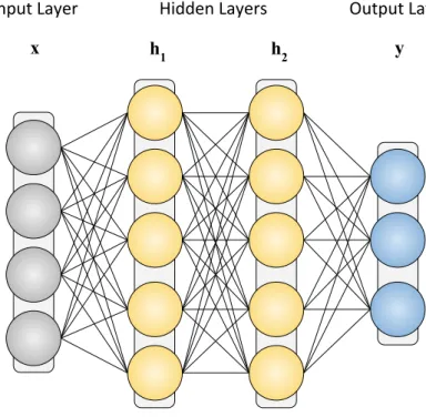
In this section, we introduce the basic concepts and the useful notation for specifying a neural network. As an example, we consider the feedforward network in Figure 3.1, which is also called Multilayer Perceptron (MLP). This network is composed by four sets of units arranged in layers: the input layer, two hidden layers, and the output layer. Every unit in a layer is connected to every other unit in the next layer, except for the output
22 Neural Networks for Sentence Modeling
Input Layer
x
Hidden Layers Output Layer
y h
1 h2
Figure 3.1: The Multilayer Perceptron (MLP), a feedforward network with two hidden layers.
layer, which represents the final output of the network. The MLP, denoted as f(x), can be mathematically described with vector-matrix operations. The input layer coincides with the x vector, and the output layer is denoted as yˆ. The hidden and output layer values are obtained by a linear transformation of the values from the previous layer. For example, the first hidden layer is computed by multiplying the input vector with a weight matrix, and adding a bias vector to the result. In our case, the full network is specified by the following equations:
ˆ y=f(x) =o(h2(h1(x)) h1(x) = σ(W1x+b1) h2(x) = ρ(W2x+b2) o(x) = W3x+b3 x∈Rdin,ˆy∈ Rdout, f :Rdin →Rdout, W1 ∈Rd1×din,b1 ∈Rd1,W2 ∈Rd2×d1,b2 ∈Rd2,W3 ∈Rdout×d1,b3 ∈Rdout
where din and dout represent the input and output dimensions respectively, while σ and ρ
are element-wise non-linear functions. These functions are applied after a linear transfor-mation. Without them, the network would consist in a sequence of linear transformations,
Neural Networks 23
Logistic (or sigmoid) f(x) = 1+1−x Hyperbolic Tangent (tanh) f(x) = 1+2−2x −1 Rectified Linear Unit (ReLU) f(x) = max(0, x) Softmax f(x)i= PKexi
k=1exk
fori= 1, ..., K
Table 3.1: Common activation functions.
which is still equivalent to a linear transformation. Therefore, the network would not be able to perform non-linear computations and learn complex functions. Theσ and ρ func-tions may be different, but often the same non-linear activation is used across the hidden layers. The output vector yˆ will contain unnormalized values also called logits. The specific nature of the learning problem usually guides the choice of some network details such as the number of outputs, the optional logit normalization function, and the loss to minimize.
3.1.1 Activation Functions
The choice of the activation function can have a substantial impact on the training process and on the final network performance. An activation function should be non-linear for allowing the network to learn complex functions — an MLP has sufficient power to act as an universal function approximator [Hornik et al., 1989]. A well behaved activation function should also be differentiable and have non-zero gradients almost everywhere.
Table 3.1 contains some common activation functions. The logistic function can be used to squash values between 0 and 1, and to model the probability of a single outcome in a network with one output unit. The tanh function outputs values between -1 and 1. The ReLU function [Nair and Hinton, 2010] keeps the positive part of the argument, and it is considered the default choice for hidden layer activation functions [Goodfellow et al., 2016]. The softmax function is often applied to the final output of a neural network in order to obtain a probability distribution out of a vector of logits. This is useful to model the probability ofK different outcomes.
3.1.2 Training the Network
The output of a neural network, such as the MLP in Figure 3.1, depends on the input and on the parameters of the network, e.g., the weight matrices and bias vectors. These parameters are fixed during inference, but need to be tuned during training in order to find a configuration that minimizes the empirical risk on the training instances. The learning process happens in two steps: the forward and backward passes.
24 Neural Networks for Sentence Modeling
During the forward pass, the network output is evaluated for a given instance under the current parameter configuration. The result is compared with the desired output, usually determined by the gold labels associated with the training instances. The comparison produces an error measure called loss, which is used as feedback during the backward pass for applying small changes to the network parameters. The goal of this process is to reduce the loss at the next iteration, and thus make the network output closer to the desired output.
3.1.3 Loss Functions
During training, the network output is compared with some ground truth using a loss function that returns a numeric value representing the network error. It is of great im-portance to select the right loss for a given task. Such choice is certainly affected by the network output type, which could be a continuous value, or an outcome out of many. In the first case, a suitable loss function would be the Root Mean Squared Error (RMSE):
RMSE =
r Pn
i=1(ˆyi−yi)2
n , (3.1)
where ˆy is the output of the network and y is the ground truth. In the second case, in which most NLP problems tackled in this thesis fall, an appropriate loss would be the categorical cross-entropy. This loss is used when we want to classify an input instance into one of possible classes. The cross-entropy measures the divergence between two probability distributions: the probability distribution produced by the network, and the ground truth probability distribution, which is usually encoded as a vector containing zeros, except for the value corresponding to the gold category, which is set to one. Such encoding is also known as one-hot label encoding. Therefore we have:
XENT =−1 n n X i=1 [yilog(ˆyi) + (1−yi) log(1−yˆi)] =− 1 n n X i=1 m X j=1 yijlog(ˆyij), (3.2)
wherey is the one-hot encoded label vector andyˆ contains the result of transforming the network logits into a valid probability distribution with the softmax function.
3.1.4 Backpropagation
Once the network and the loss function are defined, the model parameters need to be updated in such a way that the error computed by the loss function is reduced. The backward propagation or backpropagation [Rumelhart et al., 1986] is an algorithm to iteratively adjust the parameters of the network while reducing the loss. Such algorithm is based on the computation of the gradient of the loss function with respect to the
Word Representations and the Sentence Matrix 25
network parameters. Optimization algorithms based on gradient descent can use the gradient to update the network weights. Stochastic Gradient Descent (SGD) is a popular algorithm that draws a batch of examples from the training set, computes the gradients on that batch, and accordingly updates the weights [Bottou, 2010]. Adaptive optimization methods [Duchi et al., 2011; Kingma and Ba, 2014] are also popular, since they provide a faster convergence rate at the small cost of computing additional statistics.
3.2
Word Representations and the Sentence Matrix
In many machine learning algorithms, the words of a sentence are treated as symbols, and are encoded into features which signal the presence of the corresponding words or groups of words in that sentence. These features may be represented as boolean flags in the feature vector, or as continuous values capturing some occurrence statistic. These approaches for encoding words and sentences are not the best for deep learning models. Indeed, the standard way to feed textual data in neural networks is to map words into dense low dimensional representations, and build a sentence matrix. In turn, the word vectors or embeddings are obtained from the output of neural models trained with one of the following purposes: language modeling or word co-occurence prediction. Here we discuss how word embeddings are obtained, and how sentences are typically encoded.
3.2.1 Word Representations from Language Models
Language models are statistical models that try to accurately estimate the distribution of natural language sentences. Neural language model use neural networks to perform this estimation. In Bengio et al. [2003], the neural language model is trained by predict-ing the next word, given a sequence of previous words. Input words are represented as vectors having a fixed dimensionality. A feedforward neural network computes the joint probability function of word sequences, and it is trained by minimizing the negative log-likelihood of the training data. A feedforward network can condition its prediction on a fixed number of words. More powerful language models use recurrent networks [Mikolov et al., 2010], which can mantain a longer history of words seen so far. After the training converges, the tuned dense word vectors can be used in other models to represent the corresponding words.
3.2.2 Word Representations from Co-occurence Prediction
A different method for obtaining informative word embeddings consists in predicting word co-occurrence from large collections of documents. In this case, the task changes
26 Neural Networks for Sentence Modeling
Figure 3.2: The CBOW and Skip-gram models [Mikolov et al., 2013b].
to predicting a word, given some of its adjacent words. Word2vec [Mikolov et al., 2013b] and GloVe [Pennington et al., 2014] are standard methods for learning word embeddings. Word2vec has two variants (Figure 3.2): the Continuous Bag-Of-Words (CBOW) model, where a word is predicted given a fixed window of adjacent words, and the Skip-gram model, where the words in a context are predicted given a word picked from that context. GloVe is a global log-bilinear regression model which exploits word co-occurrence statistics from the corpus in the optimization function.
3.2.3 Word Embedding and Sentence Matrices
Before training a neural model, a vocabulary V is induced from the textual data that will be processed by the network. The set of pretrained word vectors and the induced vocabulary V are then used to construct a word embedding matrix. This matrix is useful to lookup a word symbol into its corresponding dense representation, and it is built by concatenating the vectors associated with all the words contained in V. Words that are not in the vocabulary may be mapped to a special UNK token, and therefore to the same random vector. Alternatively, they can be mapped to different random vectors specifically allocated for each word.
When we do text classification or passage reranking, the input to our neural network is typically a sentence s: a sequence of words (wi, .., w|s|) drawn from the vocabulary V.
Each word in the sequence is looked up in the word embedding matrix W∈Rd×|V|, and
mapped to a distributional vector w ∈ R1×d. The words in V are mapped to indices
Neural Bag-Of-Words 27
of the W matrix. Therefore, each input sentence s is converted into a sentence matrix
S∈Rd×|s|, where each columni contains the embeddingw
i associated with thei-th word
in the sentence: S= | | | w1 . . . w|s| | | |
After this, a neural network can apply a range of different transformations to the matrix in order to extract higher-level interactions between words and semantic features. More complex sentence encoding may include additional information, such as syntactic features, subword and character-based word embeddings [Alexandrescu and Kirchhoff, 2006; Sperr et al., 2013; Botha and Blunsom, 2014; Dos Santos and Zadrozny, 2014].
3.3
Neural Bag-Of-Words
In many neural models there is a point where the sentence is mapped into a single vector of continuous values. A suitable and simple approach for such a mapping is to aggregate word embedding vectors across dimensions. In Kalchbrenner et al. [2014], the sum is selected as the aggregation operation. More recent empirical results show the superiority of the averaging operation (see Deep Averaging Networks [Iyyer et al., 2015]). In this case, the word embeddings from a sentence are averaged:
z= 1 |s| |s| X i=0 wi, (3.3)
and passed through a stack of non-linear layers before producing the final output. Sentence encodings which aggregate word vectors in this way do not preserve information about word order. For this analogy with bag-of-words models, they are also referred to as Neural Bag-Of-Words (NBOW) encodings.
3.4
Recurrent Networks
The NBOW encoding is fast and simple, but starts to be less effective when embedding long sentences or entire documents, since a high number of vectors is condensed into a single one. For longer pieces of text, other encoding mechanisms can be more appropri-ate. Given that sentences can be modeled as sequences of words, methods developed for sequential data can be considered.
28 Neural Networks for Sentence Modeling
Recurrent Neural Networks (RNNs) [Elman, 1990] are one of the main approaches for modeling sequences, and they have been widely adopted for NLP tasks. Vanilla RNNs consume a sequence of vectors one step at the time, and update their internal state as a function of the new input and their previous internal state. For this reason, at any given step, the internal state depends on the entire history of previous states. These networks may suffer from the vanishing gradient problem [Bengio et al., 1994], which is mitigated by a popular RNN variant, the Long Short Term Memory (LSTM) network [Hochreiter and Schmidhuber, 1997]. An LSTM can control the amount of information from the input that affects its internal state, the amount of information in the internal state that can be forgotten, and how the internal state affects the output of the network.
Given a sequence of word embeddings (x1, ..., xT) ∈ Rdin, a cell and state vector
ct, ht ∈ Rd1 are computed for each element of the sequence by iteratively applying the
following equations, where h0 =c0 = 0:
ot=σ(Woxt+Voht−1+bo) ft=σ(Wfxt+Vfht−1+bf) it=σ(Wixt+Viht−1+bi) gt= tanh(Wgxt+Vght−1+bg) ct=ftct−1+itgt ht=ottanh(ct)
TheW, V matrices and the bvectors are parameters of the model. denotes element-wise (Hadamard) multiplication. σ is the logistic function and tanh is the hyperbolic tangent function. ot, ftanditare referred to as output, forget and input gates respectively,
since their values are bounded between 0 and 1, and control the rescaling of vectors. The Gated Recurrent Unit (GRU) [Chung et al., 2014] is an LSTM variant with similar performance and less parameters, thus faster to train. In the following equations,stdefines
the state at timestep t. Given a sequence of input vectors, the GRU computes a sequence of states (s1, ..., sT) according to:
z =σ(xtUz +st−1Wz)
r=σ(xtUr+st−1Wr)
h= tanh(xtUh+ (st−1r)Wh)
st = (1−z)h+zst−1
This recurrent unit has an update, z, and reset gate,r, and does not have an internal memory beside the internal state. The U and W matrices are parameters of the model.
![Figure 3.2: The CBOW and Skip-gram models [Mikolov et al., 2013b].](https://thumb-us.123doks.com/thumbv2/123dok_us/9898228.2483326/42.892.171.673.176.494/figure-the-cbow-and-skip-gram-models-mikolov.webp)
![Figure 3.3: A Siamese network with CNN encoders [Chopra et al., 2005].](https://thumb-us.123doks.com/thumbv2/123dok_us/9898228.2483326/47.892.220.733.190.601/figure-siamese-network-with-cnn-encoders-chopra-et.webp)
![Table 3.4: Comparison between the accuracies of the models in Wang et al. [2017] and our models (trained with the joint loss), for the paraphrase identification task (Quora).](https://thumb-us.123doks.com/thumbv2/123dok_us/9898228.2483326/55.892.266.685.193.527/table-comparison-accuracies-models-models-trained-paraphrase-identification.webp)
![Figure 4.1: The architecture of WebCrow [Barlacchi et al., 2014b].](https://thumb-us.123doks.com/thumbv2/123dok_us/9898228.2483326/60.892.276.571.191.513/figure-architecture-webcrow-barlacchi-et-al-b.webp)