Classifier combination systems and their application in human language technology

(1)

Classifier Combination Systems

and their Application

in Human Language Technology

László Felföldi

Research Group on Artificial Intelligence

May 2008

A dissertation submitted for the degree of doctor of philosophy of the University of Szeged

University of Szeged

Doctoral School in Mathematics and Computer Science

Ph.D. Programme in Informatics

(2)

(3)

Preface

For years, the pattern recognition community has focused on developing optimal learn-ing algorithms that can produce very accurate classifiers. However, experience has shown that it is often much easier to find several relatively good classifiers instead of one single very accurate predictor. The advantages of using classifier combinations instead of a single one are twofold: it helps reducing the computational requirements by using simpler models, and it can improve the classification performance.

Most Human Language Technology applications are based on pattern matching algorithms, thus improving the performance of the pattern classification has a positive effect on the quality of the overall application. Since combination strategies proved very useful in reducing classification errors, these techniques have become very popular tools in applications such as Speech Technology and Natural Language Processing.

The aim of this dissertation is basically to investigate suitable combination tech-niques for Human Language Technology applications. We propose a novel combiner algorithm based on the Analytical Hierarchy Process, and apply diﬀerent ensembles in Speech Technology and Natural Language Processing in order to improve their perfor-mance.

The first of my acknowledgements goes to my supervisor, Prof. János Csirik for supporting my research and letting me work at an inspiring department, the Research Group on Artificial Intelligence. Secondly, I would like to thank András Kocsor for the fruitful discussions and for encouraging me to pursue my studies. My heartfelt thanks goes to all my colleagues in the Speech Technology Team, who offered an invaluable amount of help and assistance in getting the results presented in this dissertation. I would also like to express my gratitude to David P. Curley for scrutinizing and correcting this dissertation from a linguistic point of view.

László Felföldi, May 2008.

(4)

(5)

Notations used

M number of classes

N number of patterns in the database

R number of classiﬁers

T number of iterations (for Bagging a Boosting)

Ci the ith classiﬁer

I the learning algorithm that creates classiﬁers _Ci

x _{a pattern}

x(i) _{feature vector of pattern} _x_{, employed by the} _i_{th classiﬁer} _C

i

x_i _the _i_{th pattern of the database}

ωj the jth class label

yi the label (or its numeric representation) of the ith pattern

wi the weight of the ith classiﬁer in linear combinations

(6)

(7)

List of Figures

1.1 The general model of a pattern recognition system. . . 2

1.2 Parallel combination scheme . . . 3

1.3 Cascading combination scheme . . . 3

1.4 Hierarchical combination scheme . . . 3

1.5 Information levels of a typical classiﬁer . . . 4

3.1 A simple AHP hierarchy. In practice, many criteria have one or more lay-ers of subcriteria. These are not shown in this simpliﬁed diagram. Also, to avoid clutter in AHP diagrams, the lines between the alternatives and criteria are often omitted or reduced in number. . . 22

4.1 The three-state left-to-right phoneme HMM. . . 32

4.2 Modular structure of the OASIS Speech Lab . . . 33

6.1 Vocal Tract Length and its frequency shifting. The graph drawn with solid and dashed line shows the spectrum of a vowel uttered by a man and a girl, respectively. . . 48

6.2 Examples of VTL warping functions. The ﬁgures show the mapping between the original (horizontal axis) and the warped (vertical axis) frequencies. . . 49

7.1 Classiﬁcation error of Bagging and Boosting algorithm on the training and training datatsets ( dashed: Bagging, solid: Boosting). . . 61

8.1 A parsing tree of a Hungarian sentence (with its English equivalent) from the Szeged Corpus “Short Business News” . . . 65

8.2 A tree pattern learning example. . . 67

(8)

(9)

List of Tables

3.1 Classiﬁer sets for thespeech and letter databases. . . 27

3.2 Classiﬁer sets for thesatimage database. . . 28

3.3 Classiﬁcation errors [%] on the Speech database (Error without combi-nation: 12.92%) . . . 28

3.4 Classiﬁcation errors [%] on the Letter database (Error without combi-nation: 13.78%) . . . 28

3.5 Classiﬁcation errors [%] on the Satimage database. (Error without com-bination: 12.05%) . . . 29

5.1 Classiﬁcation errors of the individual classiﬁers . . . 43

5.2 Combination error obtained using the Product Decision Rule . . . 44

5.3 Classification error of hybrid combinations using ANN, SVM, and kNN 45 5.4 Classification error of Bagging classifiers . . . 45

5.5 Classiﬁcation error of Boosting classiﬁers . . . 46

6.1 Recognition accuracies of the standalone classiﬁers (in percent). The parameter estimation of LD-VTLN requires all pattern data in advance, thus this method cannot be utilized in real recognition systems, its performance can be regarded as a reference value for the other normal-ization techniques. . . 52

6.2 Recognition accuracy on the databases with combination (in %). The various bars in each triplet correspond to the databases, and bar-triplets represent the applied combiner. . . 53

7.1 Accuracy of the baseline tagger and the TBL tagger. . . 57

7.2 Results achieved by various Hungarian POS taggers. . . 57

8.1 Results achieved by combining RGLearn parsers . . . 69

C.1 The relation between the thesis topics and the corresponding publications 87

(10)

(11)

1

Multiple-Classifier Systems

In this chapter we will review the most common classifier combination techniques used by the researchers today. In the literature a fair number of combination strategies have been proposed [22][52][59], these schemes differing from each other in their architec-ture, the characteristics of the combiner, and the selection of the individual classifiers. The first section will provide a general overview of these schemes, concentrating on their architecture and data representation, and discuss some of the techniques for gen-erating an effective set of classifier instances for building combinations. After discussing the basic issues of multiple classifier systems, we will overview some of the static com-bination rules applied in Human Language Technology like the “Majority Voting” and “Product” rule.

1.1 Pattern Recognition

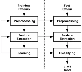
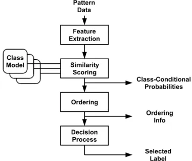
Pattern recognition (or classification) is the field of applications that seeks to learn from a given set of examples how to classify new data into a finite set of categories that are called classes. The input of a common pattern recognition system is thus an entity called a pattern (like a segment of speech signal or an image) which we would like to associate with an output class. A pattern recognition system is ususally divided into three main parts, namely preprocessing, feature selection or extraction, and classification. A pattern is represented by a set of measurements that should contain relevant information about the structure of the object that we wish to classify. The measurements can potentially be collected from a large number of data sources, which would result in a high dimensionality vector of measurements. An overall view of the main stages of a pattern recognition system is shown in Figure 1.1. The training examples (or training patterns) are the known instances from which we wish to learn a model that can generalize to previously unseen data.

Given inﬁnite training data, consistent classiﬁers approximate the Bayesian decision

(16)

2 Multiple-Classiﬁer Systems

Figure 1.1: The general model of a pattern recognition system.

boundaries to arbitrary precision, therefore providing a similar generalization. However, often only a limited portion of the pattern space is available or observable. Given a finite and noisy data set, different classifiers typically provide different generalizations. It is thus necessary to train several classifiers when dealing with classification problems so as to ensure that a good model or parameter set is found.

1.2 Multiple-Classiﬁer Systems

Given a set of independent inducers, the simplest way of building a classifier system is to select one with the best behaviour on a given testing database. During the classification just the output of the selected classifier is computed, and only this will affect the resulting decision. This selection is an “early” combination scheme widely used in Pattern Recognition.

However, selecting such a classifier is not necessarily the ideal choice since poten-tially valuable information may be wasted by discarding the results of the other clas-sifiers. In order to avoid this kind of loss of information, the output of each available classifier should be examined for making the final decision.

1.2.1 Combination Architectures

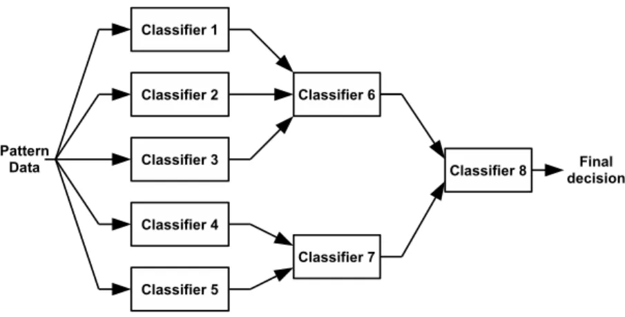
To integrate the output of several classiﬁers into a ﬁnal decision, various combination architectures are available. These architectures fall into the following three main groups:

• Parallel: Each of the inducers are invoked independently, and their results are then combined by a combiner. The majority of combination architectures in the literature belong to this category.

• Cascading: Individual classiﬁers are invoked in a linear sequence. The number of possible classes for a given pattern is gradually reduced as more classiﬁers

(17)

1.2 Multiple-Classiﬁer Systems 3

Figure 1.2: Parallel combination scheme

in the sequence are invoked. For the sake of efficiency, inaccurate but cheap classifiers are applied first, followed by more accurate and expensive inducers.

Figure 1.3: Cascading combination scheme

Cascading architectures, for instance, are commonly used in POS tagging [47] and NP parsing [102] applications.

• Hierarchical: Individual classifiers are combined into a structure similar to that of a decision tree classifier. The tree nodes, however, may now be associated with complex classifiers requiring a large number of features. The advantage of this architecture is its high efficiency and flexibility in exploiting the discriminant power of different types of features.

Figure 1.4: Hierarchical combination scheme

A number of classiﬁcation schemes like Stacking [122] and dynamic selection use this type of architecture, and have became popular in Human Language Technology applications [110].

(18)

1.2.2 Types of Knowledge Sources

The goal of designing a combination scheme is to assign a class label for an input pattern using the information coming from the individual classiﬁer instances. Each of the trained inducers has to be capable of providing the label that it prefers, but a number of machine learning methods can supply much more information than this. The combination strategies can incorporate the following types of classiﬁers based on the kind of information they provide:

Figure 1.5: Information levels of a typical classifier

• Abstract: Just the assigned class label is provided. Combiners which only need this information as input are, for instance, the voting combiners like Bagging and Boosting.

• Ranking: Instead of merely providing the best class label associated with the given pattern, the list of labels is supplied, ranked in order of probability. This more general information type can be used as input for combiners like the Borda count rule.

• Measurement or Confidence: In the most general case, each of the a poste-riori probabilities are provided. Combiners can aggregate these probabilities from different inducers and make a final decision. Examples of combiners which use the measurement information type are Prod, Sum, and Max Rules.

1.2.3 Generating eﬀective Classiﬁer Sets

A classifier combination is especially useful if the classifiers applied are largely indepen-dent. If this is not already guaranteed by the use of different learning sets or different learning methods, various re-sampling techniques like rotation and bootstrapping may be used to artificially create such differences.

(19)

1.3 Static Combination Schemes 5 • Rotation: The original learning set is divided into n disjoint subsets and uses diﬀerent unions of n−1 subsets as training sets. This technique is commonly used in cross validation during error estimation.

• Bootstrapping: A bootstrap sample can be generated by sampling instances from the training set with replacement, using a speciﬁed probability distribution. Examples include Bagging and Boosting.

• Generating noise: The generated classification model of an unstable classifier strongly depends on existing errors in the training database. Adding artificial errors is a way of generating a set of more or less independent classifiers, making it possible to fulfil the requirements of a combiner.

1.3 Static Combination Schemes

The simplest non-trainable combiner is probably the most commonly used in the mul-tiple classifier system community. Majority voting simply returns the class with the highest number of votes. There has been a huge amount of research on the theoretical aspects of majority voting for several decades, and, despite its simplicity it has proved to be quite efficient in most applications. Majority voting only takes into account the labels output by each individual classifier, but the natural way of making use of more information is to apply posterior probabilities for taking into account a confidence mea-sure for each classifier. In the following we will concentrate on the combinations of classifiers that provide confidence level information.

Consider a pattern recognition problem where the pattern x _{is to be assigned to}

one of mpossible classes (ω1, . . . , ωm). Let us assume that we haveRclassiﬁers, each

representing the given pattern by a diﬀerent feature vector. Next, denote this feature vector (employed by the ith classiﬁer) by x(i)_{. In the feature space each class} _ω_k _is

modelled by the probability density function p(x(i)_|_ω

k) and its a priori probability of

occurrence P(ωk).

According to Bayesian theory, for given features xi_, _i _{∈ {}₁_{, . . . , R}_} _{the pattern} x

should be assigned to class ωj with the maximal value of the a posteriori probability

such that

f(x_{) =} _ω_j_{, j} ₌_argmax

k

P(ωk|x(1), . . . ,x(R)). (1.1)

Let us rewrite the a posteriori probability using Bayes’ Theorem. Then We have

P(ωk|x(1), . . . ,x(R)) =

p(x(1)_{, . . . ,}x(R)_|_ω_k)_P₍_ω_k)

p(x(1)_{, . . . ,}_x(R)₎ . (1.2)

(20)

conditional feature distributions, so that

p(x(1)_{, . . . ,}x(R)_{) =} m X j=0 p(x(1)_{, . . . ,}x(R)_|_ω_j)_P₍_ω_j)_. _(1.3)

1.3.1 Product Rule

Let us assume that the probability distributions p(x(1)_{, . . . ,}_x(1)_|_ω

k) are conditionally

statistically independent. Then

p(x(1)_{, . . . ,}x(R)_|_ω_{k) =}

R Y

i=0

p(x(i)_|_ω_k)_, _(1.4)

and the decision rule

f(x_{) =}_ω_j_{, j} ₌_argmax

k

P(ωk)Y i

p(x(i)_|_ω_k)_, _(1.5)

or, in terms of the a posteriori probabilities generated by the respective classiﬁers,

argmax k P1−R(ωk)Y i p(ωk|x(i)). (1.6)

1.3.2 Sum Rule

In some applications it may be appropriate to assume that the a posteriori probabilities computed by the respective classiﬁers will not dramatically deviate from those of the prior probabilities. This is a rather strong assumption but it may be readily satisﬁed when the available information is highly ambiguous due to the high level of noise. In such a situation we may assume that the a posteriori probability can be expressed in the form

P(ωk|x(i)) = P(ωk)(1 +δki), (1.7)

where δki ≪1. Substituting this for the a posteriori probabilities in (1.6), we ﬁnd that

P1−R(ωk)Y i P(ωk|x(i)) = P(ωk) Y i (1 +δki). (1.8)

If we neglect terms of second and higher order, we can approximate the right-hand side and obtain the sum decision rule

f(x_{) =}_ω_j_{, j} ₌_argmax k " (1 +R)P(ωk) + X i p(ωk|x(i)) # . (1.9)

(21)

1.3 Static Combination Schemes 7

1.3.3 Max, Min Rule

The decision rules (1.6) and (1.9) constitute the basic schemes for combining classiﬁers. Many commonly used combination strategies can be developed from these rules after noting that Y i P(ωk|x(i))≤min i P(ωk| x(i)₎_≤X i P(ωk|x(i))≤max i P(ωk| x(i)₎_. _(1.10)

This inequality suggests that the product and sum combination rules may be approx-imated by the max and min operators, where appropriate. These approximations lead to the following: Max Rule: f(x_{) =}_ω_j_{, j} ₌_argmax k h (1 +R)P(ωk) +Rmax i p(ωk| x(i)₎i_, _(1.11) Min Rule: f(x_{) =}_ω_j_{, j} ₌_argmax k h P1−R(ωk) +Rmax i p(ωk| x(i)₎i_. _(1.12)

1.3.4 Median Rule

Note that using the equal prior assumption, the sum rule can be interpreted as com-puting the average a posteriori probability. It is well known that a robust estimate of the mean is the median, so it might be more appropriate to use it as the basis for the combining procedure. Adopting this leads to the following rule:

f(x_{) =}_ω_j_{, j} ₌_argmax k med i p(ωk| x(i)₎_. _(1.13)

1.3.5 Voting Rule

Hardening a posteriori probabilities P(ωk|x(i))will produce binary valued functions ∆ki

like ∆ki = ( 1 if P(ωk|x(i)) = max j P(ωj| x(i)₎ 0 otherwise, (1.14)

which results in combination decision outcomes rather than a combination of a posterori probabilities. Assuming that each a priori probability is equal, this leads to the following decision rule: f(x_{) =} _ω_j_{, j} ₌_argmax k X i ∆ki. (1.15)

Note that for each class ωk, the sum on the right hand side of (1.15) simply counts

(22)

1.3.6 Borda count

Instead of hardening a posteriori probabilities, it is possible to use modiﬁed probabilities

ρki based on ranking information.

ρki = 1 C X j:P(ωj|x(i))≤P(ωk|x(i)) , 1 (1.16)

where C is a normalization constant. This results in the following decision rule:

f(x_{) =}_ω_j_{, j} ₌_argmax k X i ρki. (1.17)

1.4 Summary

In this chapter we summarized the basic issues of multiple classiﬁer systems, and derived some of the static combination rules applied in Human Language Technology like the “Majority Voting” and the “Product” rule. Although these techniques have become popular in multiple-classiﬁer systems owing to their simplicity, they cannot be adapted to the special aspects of particular applications. For this reason, adaptive methods like additive combination schemes have become the focus of research. These techniques and their typical applications will be discussed in the next chapter.

(23)

2

The Additive

Combination Model

In this chapter we will focus on linear combination schemes likeaveraging and boosting techniques. These techniques can be adapted to the context of a particular application, and they have a theoretical basis. Also, experimental studies have shown that linear classifier combinations can definitely improve the recognition accuracy. Tumer and Ghosh showed that combining networks using single averagingreduces the variance of the actual decision boundaries close to the optimum boundary [108]. Later Fumera and Roli extended the theoretical framework for the weighted averagingrule [92]. However, due to their highly restrictive assumptions, we cannot say anything with confidence about the performance of the combiner.

This chapter is organized as follows. In the first section we give a brief overview of linear combination schemes, includingaveragingtechniques, and examine the theoretical background of these systems. In the next section we offer some strategies for setting the required coefficients. After, we describe the most commonly used algorithms for building effective ensemble systems like “Bagging” and “Boosting”.

2.1 Linear Combinations

Combiners aggregate the outputs of different classifiers to make a final decision. This aggregation depends on the kind of information that the individual classifiers can supply. As discussed in the previous chapter the classification methods can be grouped into three main categories:

1. Measurement or Confidence. The classiﬁer can model probability values for each class label. Let f_ij(x₎_{denote the output of classiﬁer} _C_j _{for class}_i_{and pattern} x_.

(24)

10

The Additive Combination Model

The linear combination method can be described by the formula

ˆ fi(x_{) =} N X j=1 wjfij(x), (2.1)

where fˆi(x₎ _{is the combined conﬁdence value, and} _w_j _{is the weighting factor of}

classiﬁer _Cj. The ﬁnal decision can be obtained by selecting the class with the

greatest probability, in accordance with the Bayesian decision principle.

2. Ranking. The classiﬁer can produce a list of class labels in the order of their probabilities. The combined position gˆi is then computed via the formula

ˆ gi(x) = N X j=1 wjgji(x), (2.2)

where g_ij(x₎_{is the position of the label}_ω_i _{in the classiﬁcation result of pattern}x

obtained by the classiﬁer_Cj. With the selection of a proper monotonic decreasing

function u, and

f_ij(x_{) =}_u₍_gj

i(x)), (2.3)

the ranking-type combination can be reduced to the conﬁdence-type scheme. 3. Abstract. The classiﬁer supplies only the most probable class label. In this case

the combination relies on the majority voting formula

ˆ_l₍x_{) = arg max}

i

X

lj(x)=i

wj, (2.4)

where lj(x₎ _{is the index of the class label calculated for pattern} x_{. Deﬁning the}

choice of f_ij(x₎ _as

f_ij(x_{) =}

(

1 lj(x) =i

0 otherwise (2.5)

leads to the reformulation of voting as a conﬁdence-type combination much like that for the ranking type.

As we showed earlier, the output of classiﬁers belonging to the Ranking or Abstract

class can be transformed to class conditional probability values. Therefore, in the following section we shall deal only with the conﬁdence-type combination, and expect the combiners to supply the class conditional probabilities.

2.2 Theoretical background

As mentioned previously, the output of the classiﬁers are expected to approximate the corresponding a posteriori probabilities if they are reasonably well trained. Thus

(25)

2.2 Theoretical background 11

the decision boundaries obtained using this kind of classiﬁer are close to Bayesian decision boundaries. Tumer and Ghosh developed a theoretical framework for analyzing the averaging rule of linear combinations [108]. Later Roli and Fumera extended this concept by examining the weighted averaging rule [92].

We shall focus on the classiﬁcation performance near these decision boundaries. Consider the boundary between class i1 and i2. The output of the classiﬁer is

fi(x_{) =}_p_i(x_{) +}_ǫ_i(x₎_, _(2.6)

where pi(x₎ _{is the real a posteriori probability of class} _i_{, and} _ǫ_i(x₎ _{is the estimation}

error. Let us assume that the class boundary x_b _{obtained from the approximated a}

posteriori probabilities

fi1(xb) =fi2(xb) (2.7)

are close to the Bayesian boundaries x∗_{, i.e.}

pi1(x ∗_{) =}_p

i2(x

∗₎_, _(2.8)

for a boundary between classi1 andi2. Additionally assuming that the estimated errors

ǫi(x) on diﬀerent classes are independently and identically distributed (i.i.d.) variables with zero mean, Tumer and Ghosh showed that the expected error of classiﬁcation can be expressed as:

E =EBayes+Eadd, (2.9)

where EBayes is the error of a classiﬁer with the correct Bayesian boundary. Theadded error Eadd can be expressed as:

Eadd = sσ2 b 2 , (2.10) where σ2 b is the variance of b, b = ǫi1(xb)−ǫi2(xb) s , (2.11)

andsis a constant term depending on the derivatives of the probability density functions at the optimal decision boundary.

Let us consider the eﬀect of combining multiple classiﬁers. We shall deal only with linear combinations, so we have the following combined probabilities:

ˆ fi(x_{) =} N X j=1 wjfij(x), (2.12)

(26)

12 The Additive Combination Model weights, i.e. N X j=1 wj = 1, wj ≥0 (2.13) we have that ˆ fi(x_{) =}_p_i(x_{) + ˆ}_ǫ_i(x₎_, _(2.14) where ˆ ǫi(x_{) =} N X j=1 wjǫji(x) (2.15)

Let us compute the variance ofˆb, where

ˆ_b₌ ˆǫi1 −ˆǫi2

s . (2.16)

Assuming that ǫj_i(x₎ _{are i.i.d. variables with zero mean and variance} _σ2

ǫj, the errors of

different classifiers on the same class are correlated, while on different classes they are uncorrelated. Cov(ǫm_i₁(x_b)_{, ǫ}n i2(xb)) = ( ρmn wheni1 =i2 0 otherwise ,

where ρmn denotes the covariance between the errors of classiﬁer Cm and Cn for each

class. Expanding the tag σ2

ǫ in Eq. (2.10), we ﬁnd that ˆ Eadd = 1 s N X j=1 w_j2σ2_ǫj + 1 s X m6=n wmwnρmn.

Expressed in terms of additional errors of the classiﬁers

ˆ Eadd = 1 s N X j=1 w2 jE j add + 1 s X m6=n wmwnρmn,

where the term E_addj denotes the added error of the classiﬁer _Cj. In the case of

uncorrelated estimation errors (i.e. when ρmn= 0), this equation reduces to

ˆ Eadd= N X j=1 w_j2E_addj , (2.17)

(27)

2.3 Simple Adaptive Combinations 13

which leads to the following optimal values for w:

wj =c 1

E_addj , (2.18)

where c is a normalization factor. With equally performing classiﬁers, that is when all the errors E_addj have the same value

E_addj =Eadd, j= 1, . . . , N, (2.19)

we obtain the Simple Averaging rule:

wj = 1

N, (2.20)

which results in the following error value:

ˆ

Eadd = 1

NEadd. (2.21)

This formula shows that, under the conditions mentioned, linear combinations reduce the error of the individual classiﬁer. Taking into account correlated errors, however, does not lead to a simple general expression for optimal values of weights, and other methods are required to estimate the optimal parameters.

2.3 Simple Adaptive Combinations

To achieve the best combination performance the parameters of the combiner can be trained on a selected training data set. The form of linear combinations we deal with is quite simple, the trainable parameters being just the weights of classiﬁers. Thus the various linear combinations diﬀer only in the values of these factors. In the following we give some examples of methods commonly employed, and in the next section we propose a new method for computing these parameters.

1. Simple Averaging. In this simplest case, the weights can be selected so they have the same value:

wj = 1

N. (2.22)

As mentioned before, this selection is optimal when all the classiﬁers have a very similar performance, and all the assumptions mentioned in Section 2.2 hold.

2. Weighted Averaging. Experiments show [92] thatSimple Averaging can be out-performed when selecting weights to be inversely proportional to the error rate of the corresponding classiﬁer:

wj = 1

Ej

(28)

14

where Ej is the error rate of the classiﬁer Cj, i.e. the ratio of the number

of correctly classiﬁed patterns and total number of patterns on a selected data set for training the combiner. This rule (a more general version of the Simple Averaging rule) is employed in order to handle the combination of unequally performing classiﬁers.

3. Hierarchical methods. To calculate the weightswj one can take those values that

minimize some kind of distance between the computed and required conditional scores: min w X x∈X l X i=1 L( ˆfi(x₎_{, r}_i))_, _(2.24)

where ri is the requested conditional scores for class i, and L( ˆfi(x), ri)) is the

loss function. Since machine learning algorithms can be regarded as optimization methods that minimize the expected value of a loss function on the training database, this optimization can be done by applying an appropriate machine learning algorithm.

2.4 Bagging

The Bagging (Bootstrap aggregating) algorithm[16] votes classiﬁers generated by dif-ferent bootstrap samples (replicates). A bootstrap sample is generated by uniformly sampling m instances from the training set with replacement. T bootstrap samples

B1, B2, ..., BT are generated and a classiﬁerCi is built from each bootstrap sample Bi.

A ﬁnal classiﬁer C∗ _{is built from}_C

1,C2, ...,CT whose output is the class predicted most

often by its sub-classiﬁers (majority voting).

Algorithm 1 Bagging algorithm Require: Training Set S, Inducer I Ensure: Combined classifier _C∗

for i= 1. . . T do

S′ _{= bootstrap sample from} _S Ci =I(S′) end for C∗₍_x_{) =}_argmax j X i:Ci(x)=ωj 1

For a given bootstrap sample, an instance in the training set will have a probability

1−(1−1/m)m of being selected at least once from theminstances randomly selected from the training set. For large m, this is about 1-1/e = 63.2%. This perturbation causes different classifiers to be built if the inducer is unstable (e.g. ANNs, decision trees) and the performance may improve if the induced classifiers are uncorrelated. However, Bagging can slightly degrade the performance of stable algorithms (e.g. kNN) since effectively smaller training sets are used for training.

(29)

2.5 Random Forests 15

2.5 Random Forests

Breiman proposed Random Forests [15] as a variant of Bagging. A random forest is an ensemble creation method that uses tree classifiers like C4.5 algorithm as a base classifier. An ensemble of decision trees is built by generating independent identically distributed random vectors Θj, j = 1, ..., K. One tree is grown from each vector. The difference with Bagging is that the vectors Θj can be built by sampling from feature sets, a sample set or by varying some parameters of the tree (e.g. the number of nodes). In /citeRodriguez, Rodriguez et al. proposed a variation of random forest called Rotation forests that simply adds a PCA pre-processing in order to decorrelate the training data. They showed that experimental improvements could be obtained on many datasets.

2.6 Boosting

The underlying idea of boosting is to combine simple rules iteratively to form an en-semble that will improve the performances of each single member. Boosting theory has its roots in Probably Approximately Correct (PAC) learning [112]. PAC gives a nice formalism for deciding how much training data we need in order to achieve a given prob-ability of correct predictions on a given fraction of future test data. In [112], Valiant showed that simple rules, each performing only slightly better than random guessing, can be combined to form an arbitrarily good ensemble. The challenge of boosting is to ﬁnd a PAC algorithm with arbitrarily high accuracy.

The ﬁrst boosting algorithms were proposed by Schapire in 1990 [94] and Freund in 1995 [30]. However, several strong assumptions prevented the eﬃciently use of these algorithms in practical situations: They need prior knowledge of the accuracy of the weak hypotheses.

2.6.1 Adaboost

A ﬁrst step towards more practical Boosting is the AdaBoost (Adaptive Boosting) algorithm [31]. Adaboost is adaptive in the sense that a new hypothesis is selected given the performances of the previous iterations. Unlike bagging, this allows the algorithm to focus on the hard examples. This adaptive strategy is managed by a weight distribution D over the training samples. A weight D(i)is given to each training pattern x_i_{. Examples with large weights will have more impact on choosing the weak}

hypothesis than those with low weights. Then after each round, the weight distribution is updated in such a way that the weight of misclassiﬁed examples is increased.

In the following we shall deal with only the case of binary classiﬁcation, i.e. only two class labels {−1,+1}are available. Let us consider, as usual, a training set ZN = (x₁_{, y}₁₎_,₍x₂_{, y}₂₎_{, ...,}₍x_N_{, y}_N₎_{. We suppose that we have a base learning algorithm (or}

weak learner) which accepts as input a sequence of training samples Zn along with

(30)

16

constructs a weak hypothesis C. The predicted label y is given by sign(C(x₎₎_{, while}

the conﬁdence of the prediction is given by kC(x₎_k_{. We shall also assume that the}

corresponding weighted training error is smaller than 1/2. This means that the weak hypotheses have to be at least slightly better than random guessing with respect to the distribution D. The distribution D is ﬁrst initialized uniformly over the training samples. Then it is iteratively updated in such a way that the likelihood of the objects beeing misclassiﬁed in the previous iteration is increased.

The loss function L used for updating the weights (step 4 in the main loop) is usually an exponential loss function, but other loss functions have been also proposed in the literature (Logitboost [32] or Arcing [14]).

Two critical choices in AdaBoost are how to choose the weak hypothesis _Ct and

what is the optimal wt. Let us deﬁne the training error of the ensemble Cˆ:

L1/0( ˆC) = 1 N n X i=1 L1/0(yi,C(xi)), (2.25)

where L1/0 is the1/0 loss function

L1/0(yi,C(xi)) = (

1 if yi =C(xi)

0 otherwise (2.26) Shapire and Singer [95] give a bound on the training error of the combined hypothesis

ˆ C: L1/0( ˆC)≤ T Y t=1 Nt, (2.27)

where Nt=P_iDitexp(−ωtyiCt(xi)).

According to this theorem, the training error can be minimized by greedily minimiz-ing Nt on each round of boosting. To choose the optimal ωt, we will consider several

cases in the following sections.

2.6.2 Discrete Adaboost

Let us ﬁrst consider the original version of AdaBoost, called Discrete AdaBoost, when the range of each weak hypothesis is restricted to the labels _{−1,+1_}. Then the optimal ωt can be found by approximatingNt as follows:

Nt = X i D_itexp(₋ωtyiCt(xi)) (2.28) ≤ X i Dt i 1 +yiCt(xi) 2 exp(−ωt) + 1₋yiCt(xi) 2 exp(ωt) . (2.29)

(31)

2.6 Boosting 17 Algorithm 2 Boosting algorithm

Require: Training SetZN = (x1, y1),(x2, y2), ...,(xN, yN), number of iterationsT,

Inducer I

Ensure: Combined classifier C∗

Dn(1) = 1/N for all n = 1, . . . , N.

for t= 1. . . T do

S′ _{= bootstrap sample from} _Z

N with distribution Dnt Ct=I(S′) ǫt= _n1 PNn=1L1/0(yn,C(xn)) ifǫt>1/2then Exit select optimal wt update weights D(nt+1) = D (t) n L(yn,C(xn)) Nt ,

whereNt is a normalization factor such that PNn=1D (t+1)

n = 1.

end for

C∗₍_x_{) =}_sign₍PT

t=1wtCt(x))

The coeﬃcient wt that minimizes Nt can be found analytically:

wt = 1 2log 1 +rt 1−rt , (2.30) where rt = P

iDityiCt(xi). With this choice of coeﬃcient, the training error of the

combined hypothesis _Cˆis bounded by:

L1/0( ˆC)≤ T Y t=1 p 1₋r2 t. (2.31)

The quantity rt is a natural measure of the correlation of the predictions ofCt and the

labels yi with respect to Dt. From equation 2.31 it follows that:

L1/0( ˆC)≤exp − T X t=1 r_t2 ! , (2.32)

from which we infer that the condition PT

t=1rt2 → ∞ suﬃces to guarantee that the

training error converges towards 0 when the number of iteration increases. Clearly this holds if rt ≥ r0 > 0 for some positive constant r0 (recall that the weighting training

error of a weak hypothesis is less than 0.5).

2.6.3 Real Adaboost

A more general formulation of Discrete AdaBoost uses the confidence levels of each weak classifier instead of just binary outputs. It is called Real AdaBoost [95]. Unlike Discrete AdaBoost, the output space of the weak classifiers is not restricted to{−1; 1}, but can take values in R. More specifically, let us consider a partition of R into disjoint

(32)

18

blocks X1, X2, ..., Xn for which h(x′) = h(x) = cj for all (x,x′) ∈ Xj ×Xj . Let

us further assume that the partitioning is given. The task is to ﬁnd the optimal cj ,

j = 1, ..., N. Let

W_j+ = X i:xi∈Xj,yi=+1

Di (2.33)

be the weighted fraction of positive samples falling into partition Xj, and

W−

j =

X

i:xi∈Xj,yi=−1

Di (2.34)

the equivalent for the negative class. Then the normalization factorNtcan be rewritten

as:

Nt = X

j

(W_j+exp(−cj) +W_j−exp(cj)). (2.35)

The expression that we want to minimize has the optimal cj values

cj = 1 2log W_j+ W_j− ! (2.36)

This technique has proved to be very effective in many applications, outperforming Discrete AdaBoost by taking into account the confidence measures of the weak hy-potheses. A good example of a weak learner that can be used using this partitioning technique is a simple decision tree. The leaves of the tree directly define the partition of the domain.

Note that in practice,W_j+orW_j−is very small, which could produce an inconsistency in Equation 2.36. That is why we generally use a smoothed version of the coeﬃcients:

cj = 1 2log W_j++ǫ W_j−+ǫ ! , (2.37)

where ǫ >0 is an appropriately small positive-valued constant.

2.6.4 Generalization error

So far have we only considered training error convergence to demonstrate the eﬃciency of AdaBoost, but minimizing the empirical risk is no guarantee of a good generalization. However, in practical situations, AdaBoost seems very unlikely to overﬁt and has one more interesting property: the test error continues decreasing with the number of itera-tions, even if the training error has reached zero. In order to explain this phenomenon, let us analyze AdaBoost from a margin perspective. Let us recall that the ensemble hypothesis has the form:

Without loss of generality, we can assume that PN

j=1ωj = 1. Let us call H the

space of the hypotheses ht. Similar to margins in Support Vector Machines, we can

(33)

2.7 Summary 19

can be viewed as a conﬁdence in the prediction of H. Shapire proved [95] that the generalization error is upper bounded with probability 1−δ for all θ >0and for all f

by PZn(yf(x)≤θ) +O 1 √ n dlog2(n/d) θ2 + log( 1 δ) 12! , (2.38)

wherePZN denotes the probability with respect to choosing an example(x, y)uniformly

from the training set ZN and d can be regarded as the VC dimension of H.

The bound stated in the equation does not depend on the number of classiﬁers in the ensemble, but remains quite loose in practical applications. However, it shows the tendency that larger margins lead to a better generalization. In fact, the generalization continues to improve even after the training error has reached zero because the margin is still increasing. Note that several studies have tried to interpret AdaBoost as a soft margin classiﬁers [74, 89]

2.7 Summary

In this chapter we outlined the main aspects of linear combination techniques, along with their theoretical background. We examined how to build simple adaptive combi-nation strategies and described the popular methods called “Bagging” and “Boosting”. These methods have proved effective in improving the overall classification performance, especially in the case of “weak” classifiers, but at a cost. To achieve high accuracies it may require hundreds or thousands of iterations, which limits their practical usefulness. In the next chapter we will introduce a simpler approach which works better than the simple additive models and is less CPU demanding than the sophisticated Boosting variants.

(34)

(35)

3

Combinations and the

Analytic Hierarchy Process

Linear combination schemes, especially Boosting algorithms, are frequently used in machine learning applications due to their ability to improve the classification per-formance. The Adaboost algorithm and its variants create a sequence of classifier instances by training the same classifier algorithm on special bootstrap-samples of the training database. The classification performance of the original classifier method can be dramatically increased, especially in the cases of “weak” classifers, but for the final solution it requires hundreds or thousands of iterations. In the practice, however, most of the applications cannot provide the required huge amount of resources for applying such a great number of classifier instances.

In this chapter we will presents an eﬀective combination solution for these kinds of applications. In the ﬁrst section we will give a brief summary of the Multi-criteria Decision Making and the fundamentals of the Analytic Hierarch Process. In the second section we will investigate the mathematical properties of AHP, and a novel combination method will be proposed in the third section.

3.1 Analytic Hierarchy Process

Analytic Hierarchy Process allows decision makers to model a complex problem in a hierarchical structure which showing the relationships of the goal, objectives (criteria), sub-objectives, and alternatives (See Figure 3.1). Uncertainties and other inﬂuencing factors can also be included.

AHP allows for the application of data, experience, insight, and intuition in a log-ical and thorough way. It enables decision-makers to derive ratio scale priorities or weights as opposed to arbitrarily assigning them. In so doing, AHP not only supports decision-makers by enabling them to structure complexity and exercise judgment, but

(36)

22

Combinations and the Analytic Hierarchy Process

Figure 3.1: A simple AHP hierarchy. In practice, many criteria have one or more layers of subcriteria. These are not shown in this simplified diagram. Also, to avoid clutter in AHP diagrams, the lines between the alternatives and criteria are often omitted or reduced in number.

allows them to incorporate both objective and subjective considerations into the deci-sion process. AHP is a compensatory decideci-sion methodology because alternatives that are deﬁcient in one or more objectives can compensate by their performance in other objectives. It is composed of several previously existing but unrelated concepts and tech-niques such as hierarchical structuring of complexity, pairwise comparisons, redundant judgments, an eigenvector method for deriving weights, and consistency considerations. Although each of these concepts and techniques were useful in themselves, the syner-gistic combination of the concepts and techniques (along with some new developments) produced a process whose power is indeed far more than the sum of its parts.

Users of the AHP ﬁrst decompose their decision problem into a hierarchy of more easily comprehended sub-problems, each of which can be analyzed independently. The elements of the hierarchy can relate to any aspect of the decision problem - tangible or intangible, carefully measured or roughly estimated, well- or poorly-understood-anything at all that applies to the decision at hand.

Once the hierarchy is built, the decision makers systematically evaluate its various elements, comparing them to one another in pairs. In making the comparisons, the decision makers can use concrete data about the elements, or they can use their judg-ments about the elejudg-ments’ relative meaning and importance. It is the essence of the AHP that human judgments, and not just the underlying information, can be used in performing the evaluations.

The AHP converts these evaluations to numerical values that can be processed and compared over the entire range of the problem. A numerical weight or priority is derived for each element of the hierarchy, allowing diverse and often incommensurable elements to be compared to one another in a rational and consistent way. This capability distinguishes the AHP from other decision making techniques.

In the ﬁnal step of the process, numerical priorities are derived for each of the decision alternatives. Since these numbers represent the alternatives’ relative ability to achieve the decision goal, they allow a straightforward consideration of the various courses of action.

(37)

3.2 Mathematical model 23

1. The alternatives and the signiﬁcant attributes are identiﬁed.

2. For each attribute, and each pair of alternatives, the decision makers specify their preference (for example, whether the location of alternative “A” is preferred to that of “B”) in the form of a fraction between 1/9 and 9.

3. Decision makers similarly indicate the relative signiﬁcance of the attributes. For example, if the alternatives are comparing potential real-estate purchases, the investors might say they prefer location over price and price over timing.

4. Each matrix of preferences is evaluated by using eigenvalues to check the consis-tency of the responses. This produces a “consisconsis-tency coeﬃcient” where a value of 1 means all preferences are internally consistent. This value would be lower, however, if a decision maker said X is preferred to Y, Y to Z but Z is preferred to X (such a position is internally inconsistent). It is this step that causes many users to believe that AHP is theoretically well founded.

5. A score is calculated for each alternative.

The two basic steps in the process are to model the problem as a hierarchy, then to establish priorities for its elements.

3.2 Mathematical model

To compute the importance of possible choices, pairwise comparison matrices are uti-lized for each criterion. The element aij of the comparison matrix A represents the

relative importance of choice i against the choice j, implying that the element aji is

the reciprocal of aij. Let the importance value v of choice y be expressed as a linear

combination of the importance values for each applied criterion:

v(y) = n X

j=1

wjv(yj), (3.1)

where wj is the importance of choicey with respect to the criterionyj. Using

compar-ison matrices AHP propagates the importance values of each node from the topmost criteria towards the alternatives, and selects the alternative with the greatest importance value as its ﬁnal decision.

Let us now focus on the computation of the weightswfor a selected criterion. The elements of a given pairwise comparison matrix approximate the relative importance of the choices, thus

aij ≈

wi

wj

, (3.2)

(38)

24

is called consistent if its components satisfy the following equalities:

mij = 1 mji , (3.3) and mij =mikmkj ∀ i, j, k. (3.4)

If A is not consistent, it is not possible to ﬁnd a vector wthat satisﬁes the equation

aij =

wi

wj

. (3.5)

Now let us deﬁne the matrix of weight ratios by

W =         w1 w1 w1 w2 w1 w3 · · · w1 wn w2 w1 w2 w2 w2 w3 · · · w2 wn w3 w1 w3 w2 w3 w3 · · · w3 wn ... ... ... ... ... wn w1 wn w2 wn w3 · · · wn wn         , (3.6)

or, in matrix notation,

W =wwT. (3.7)

Note that eqs. (3.3) and (3.4) hold for the matrix W:

wij = wi wj = wi wk wk wj =wikwkj, (3.8)

hence the matrix of weight ratios is consistent.

Because the rows of matrix W are linearly dependent, the rank of the matrix is

1, and there is only one nonzero eigenvalue. Knowing that the trace of a matrix is invariant under similarity transformations, the sum of diagonal elements is equal to the sum of eigenvalues, which implies that the nonzero eigenvalueλmax equals the number

of the rows:

λmax =n. (3.9)

It is straightforward to verify that the vector w is an eigenvector of matrix W corre-sponding to the maximum eigenvalue

(W w)i = n X j=1 Wijwj = n X i=1 wi wj wj = n X j=1 wi = nwi.

(39)

3.2 Mathematical model 25

The aim of AHP is to resolve the weight vectorwfrom a pairwise comparison matrix

A, where the elements of A correspond to the measured or estimated weight ratios. Following Saaty we shall assume that

aij >0, (3.10) and aij = 1 aji . (3.11)

From matrix theory it is known that a small perturbation of the coeﬃcients implies a small perturbation of the eigenvalues. Hence we still expect to ﬁnd an eigenvalue close to n, and select the elements of the corresponding eigenvector as weights. It can be proved that

λmax≥n,

and the matrix A is consistent if and only if λmax = n. A way of measuring the

consistency of the matrix A is by deﬁning the consistency index (CI) as the negative average of the remaining eigenvalues:

CI = X λ<λmax λ n−1 = λmax−n n−1 (3.12)

3.2.1 Combinations based on AHP

As mentioned above, AHP provides the following solution for the problem of linear MCDM systems: v(y) = n X i=1 wiv(yi),

where the importance value of the choice is the linear combination of the importance values of the direct criteria. In linear classiﬁer combinations the combined class condi-tional probabilities are computed as weighted sums of the probability values from each classiﬁer, so fi(x) = N X j=1 wjfij(x).

Noting the similarities between these two methods, it is clear that, by applying pairwise comparisons on classiﬁers performance, AHP provides a way of computing the weights of inducers in classiﬁer combinations. Let us calculate the elementaij of the comparison

matrix as the quotient of classiﬁcation performance on a selected test data set:

aij = 1 Ei 1 Ej = 1 aji , (3.13)

(40)

26

where Ei is the classiﬁcation error of classiﬁer Ci. If all the performance errors are

measured on the same test data set, the comparison matrix A is consistent, and the elements of the eigenvector whose corresponding eigenvalue is N, that is

wi = 1

Ei

, (3.14)

are the same those as generated byweighted averaging. However, this method allows us to make pairwise comparisons of different inducers applied on different (e.g. randomly generated) test sets, taking advantage of the stabilizing effect of AHP. This leads to a more robust classification performance, especially in noisy environments, as shown in the experiments section.

3.3 Experiments

In this section we will describe our experiments for comparing the performance of

averaging combiners and our AHP-based combiner.

3.3.1 Evaluation Domain

In the experiments three data sets were employed: a data-set used in our speech recognition system, and two other datasets (letter and satimage) originating from the statlog/UCI repository. (http://www.liacc.up.pt/ML/statlog)

1. Speech data set. The database is based on recorded samples taken from 160 children aged between 6 and 8. The ratio of girls and boys was 50% - 50%.The speech signals were recorded and stored at a sampling rate of 22050 Hz in 16-bit quality. Each speaker uttered all the Hungarian vowels, one after the other, separated by a short pause. Since we decided not to discriminate their long and short versions, we only worked with 9 vowels altogether. The recordings were divided into a train and a test set in a ratio of 50% - 50%. There are numerous methods for obtaining representative feature vectors from speech data, but their common property is that they are all extracted from 20-30 ms chunks or ’frames’ of the signal in 5-10 ms time steps. The simplest possible feature set consists of the so-called bark-scaled filterbank log-energies (FBLE). This means that the signal is decomposed with a special filterbank and the energies in these filters are used to parameterize speech on a frame-by-frame basis. In our tests the filters were approximated via Fourier analysis with a triangular weighting. Alto-gether 24 filters were necessary to cover the frequency range from 0 to 11025 Hz. Although the resulting log-energy values are usually sent through a cosine trans-formation to obtain the well-known mel-frequency cepstral coefficients (MFCC), we abandoned it because, as we observed earlier, the learner we work with is not sensitive to feature correlations so a cosine transformation would bring no significant improvement.

(41)

3.3 Experiments 27

2. Letter Data Set. The objective of the Data set is to identify each of a large number of black-and-white rectangular pixel displays as one of the 26 capital letters in the English alphabet. The character images were based on 20 different fonts and each letter within these 20 fonts was randomly distorted to produce a file of 20,000 unique stimuli. Each stimulus was converted into 16 primitive numerical attributes (statistical moments and edge counts) which were then scaled to fit into a range of integer values from 0 to 15. We typically trained on the first 16000 items and then used the resulting model to predict the letter category for the remaining 4000.

3. Satimage Data Set. One frame of Landsat MSS imagery consists of four digital images of the same scene in different spectral bands. Two of these are in the visible region (corresponding approximately to green and red regions of the visible spectrum) and two are in the (near) infra-red. Each pixel is a 8-bit binary word, with 0 corresponding to black and 255 to white. The spatial resolution of a pixel is about 80m x 80m. Each image contains 2340 x 3380 such pixels. The database is a (tiny) sub-area of a scene, consisting of 82 x 100 pixels. Each line of data corresponds to a 3x3 square neighborhood of pixels completely contained within the 82x100 sub-area. Each line contains the pixel values in the four spectral bands (converted to ASCII) of each of the 9 pixels in the 3x3 neighborhood and a number indicating the classification label of the central pixel. The number of possible class labels for each pixel is 7. We trained on the first 4435 patterns of the database and selected the remaining 2000 patterns for testing.

3.3.2 Evaluation Method

During the experiments we compared the performance of 6 different combiners applied on each of the 3 databases. For each of the databases we trained 3-layered neural networks with different structures, and selected 5 subsets of classifiers, denoted by

Set1to Set5.

In the case of the speech and letter databases we trained networks, setting the number of neurons in the hidden layer to 5, 10, 20, 40, 80, 160, and 320. Table 3.1 shows the construction of classiﬁer sets. The columns refer to the number of hidden neurons, and the rows show which networks belong to the selected classiﬁer sets.

5 10 20 40 80 160 320 Set1 x x x x x x x Set2 x x x x x x Set3 x x x x x Set4 x x x x Set5 x x x

Table 3.1: Classifier sets for the speech and letterdatabases.

(42)

28

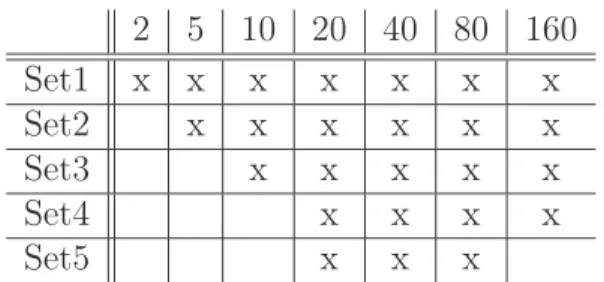
with hidden layer size set to 2, 5, 10, 20, 40, 80, and 160. The corresponding classiﬁer selection is displayed in Table 3.2.

2 5 10 20 40 80 160 Set1 x x x x x x x Set2 x x x x x x Set3 x x x x x Set4 x x x x Set5 x x x

Table 3.2: Classifier sets for the satimage database.

The experiments compared the performance of linear combination schemes with diﬀerent methods for acquiring the proper weights. We examined 2 schemes of Aver-aging : SAand W A (i.e. simple and weighted) averaging, and 4 schemes ofAHP. To calculate the pairwise comparison matrices needed for the AHP method, we took the quotient of classiﬁcation errors of the two competing networks on a random test set generated by bootstrapping (resampling the training data set with replacement) of the training set. Based on the size of the generated test set we had 4 AHP schemes,AHP1

to AHP4, setting the size of each to 50, 100, 200 and 400, respectively. With the

W A combiner, the original training set was chosen for the calculation of the weights.

3.3.3 Results and Discussion

Set1 Set2 Set3 Set4 Set5

SA 8.52 9.26 9.95 9.77 8.80 W A 8.66 9.21 9.91 9.81 8.75 AHP1 8.66 8.94 9.44 10.05 8.80 AHP2 8.56 9.12 9.72 10.19 8.80 AHP3 8.61 9.21 9.49 9.58 8.70 AHP4 8.61 9.31 9.55 9.07 8.70

Table 3.3: Classification errors [%] on the Speech database (Error without combi-nation: 12.92%)

Set1 Set2 Set3 Set4 Set5

Table 3.4: Classification errors [%] on the Letter database (Error without combi-nation: 13.78%)

(43)

3.4 Conclusions and Summary 29 Set1 Set2 Set3 Set4 Set5

Table 3.5: Classification errors [%] on the Satimage database. (Error without combination: 12.05%)

Tables 6.1, 6.2, and 3.5 show the results of our experiments. The columns represent the various classifier sets, while the rows show the classification errors measured using the selected combination of the corresponding classifier group.

As expected, However, in some casesSAperformed better thanW Aand theAHP

combiners, telling us that the strong assumptions of the method are not always satisﬁed [34].

The performance ofAHP combiners depends on the size of the testing set. When the test sets selected were too small, the measured accuracy values did not characterize the goodness of the classiﬁers, and yielded poor combination results. Increasing the size, however, makes the consistency index (CI) tend to zero, producing weights that tend to the values calculated by weighted averaging. Determining the optimal size of the test set will probably require further study.

When considering the sensitivity for the selection of different classifier subsets, the AHP-based combiner has a behaviour similar to that of the W A method, hence the optimal classifier set can be selected by methods available for the averagingcombiners [92].

3.4 Conclusions and Summary

In this chapter the Analytic Hierarchy Process was described in brief. Based on this technique the author designed and implemented a novel linear combination method, and then he compared its performance with those of other combiners. As shown in the experiments, AHP-based combinations proved an eﬀective generalization of the

weighted averaging rule; they outperformed the other averaging methods in almost every case. This dual aspect of simplicity and improved performance was the author’s original intention for devising such a method.

(44)

(45)

4

Speech Recognition

Speech recognition is a pattern classification problem in which a continuously varying signal has to be mapped to a string of symbols (the phonetic transcription). Speech signals display so many variations that attempts to build knowledge-based speech rec-ognizers have mostly been abandoned. Currently researchers tackle speech recognition only with statistical pattern recognition techniques. Here, however a number of special problems arise that have to be dealt with. The first one is the question of the recogni-tion unit. The basis of the statistical approach is the assumprecogni-tion that we have a finite set of units (in other words, classes), the distribution of which is modelled statistically from a large set of training examples. During recognition an unknown input is classi-fied as one of these units using some kind of similarity measure. Since the number of possible sentences or even words is potentially infinite, some sort of smaller recognition unit has to be chosen in a general speech recognition task. The most commonly used unit of this kind is the phoneme, hence the next chapters deal with the classification problem of phonemes.

The other special problem is that the length of the units may vary, that is utterances get warped along the time axis. The only known way of solving this is to perform a search in order to locate the most probable mapping between the signal and the pos-sible transcriptions. Normally a depth-ﬁrst search is applied (implemented by dynamic programming), but a breadth-ﬁrst search with a good heuristic is a viable option as well.

4.0.1 Phoneme Modeling

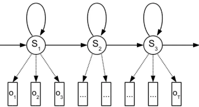
Hidden Markov Models [87] synchronously handle both the problems mentioned above. Each phoneme in the speech signal is given as a series of observation vectors

O=o1, ..., oT, (4.1)

(46)

32 Speech Recognition

and one has one model for each unit of recognition. These models eventually return a class-conditional likelihood P(O|c), where c refers to these units. The models are composed of states, and for each state we model the probability that a given observation vector belongs to (“was omitted by”) this state. Time warping is handled by state transition probabilities, that is the probability that a certain state follows the given state. The ﬁnal “global” probability is obtained as the product of the proper omission and state-transition probabilities.

Figure 4.1: The three-state left-to-right phoneme HMM.

When applied to phoneme recognition, the most common state topology is the three-state left-to-right model (see Figure refHMM). We use three states s1, s2 and s3

because the ﬁrst and last parts of a phoneme are usually diﬀerent from the middle due to coarticulation. This means that in a sense we do not really model phonemes but rather phoneme thirds.

Because the observation vectors usually have continuous values the state omission probabilities have to be modeled as multidimensional likelihoods. The usual procedure is to employ a mixture of weighted Gaussian distributions for all state sj of the form

p(ρ_|sj) = k X

i=1

αiN(σ, µi,Σi), (4.2)

where N(σ, µi,Σi)denotes the multidimensional normal distribution with meanµi and

covariance matrix Σi, k is the number of mixtures, and αi are non-negative weighting

factors which sum to 1.

A possible alternative to HMM are the Stochastic Segmental Models. The more sophisticated segmental techniques ﬁt parametric curves to the feature trajectories of the phonemes [80]. There is, however, a much simpler methodology [60][61] that applies non-uniform smoothing and sampling in order to parametrize any phoneme with the same number of features, independent of its length. The advantage of this uniform parametrization is that it allows us to apply any sort of machine learning algorithm for the phoneme classiﬁcation task. This is why we chose this type of segmental modeling for the experiments performed and also for our speech recognition system [104].

Hidden Markov Models describe the class conditional likelihoods P(O|c). These type of models are called generative, because they model the probability that an obser-vation O was generated by a classc. However, the final goal of classification is to find

(47)

4.1 The OASIS System 33

the most probable class c. We can readily compute the posterior probabilities P(c|O)

from P(O|c)using Bayes’ law since

P(c|O) = P(O|c)P(c)

P(O) (4.3)

Another approach is to model the posteriors directly. This is how discriminative learners work. Instead of describing the distribution of the classes, these methods model the surfaces that separate the classes and usually perform slightly better than generative models.

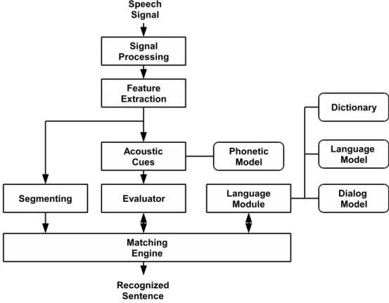
In the following chapters in the phoneme classification tests we work both with generative and discriminative methods. But before doing this we shall briefly introduce the OASIS speech recognition system [60][61], developed at the Research Group on Artificial Intelligence, which served as a framework for all the tests.

4.1 The OASIS System

The OASIS system was designed with the aim of creating a general framework that is ﬂexible enough to allow the experimentation with a wide range of techniques in speech recognition. In the following we will give a short overview of the system.

Classifier combination systems and their application in human language technology