Forecasting US bond default ratings allowing for previous and
initial state dependence in an ordered probit model
∗Paul Mizen University of Nottingham Serafeim Tsoukas University of Glasgow August 1, 2011 Abstract
In this paper we investigate the ability of a number of different ordered probit models to predict ratings based on firm-specific data on business and financial risks. We investigate models based on momentum, drift and ageing and compare them against alternatives that take into account the initial rating of the firm and its previous actual rating. Using data on US bond issuing firms rated by Fitch over the years 2000 to 2007 we compare the performance of these models in predicting the rating in-sample and out-of-sample using root mean squared errors, Diebold-Mariano tests of forecast performance and contingency tables. We conclude that initial and previous states have a substantial influence on rating prediction.
Key words: Credit ratings, probit, state dependence JEL: G24, G33, C25, C53
∗Corresponding Author: Serafeim Tsoukas, Department of Economics, University of Glasgow, Adam Smith
Build-ing, Glasgow, G12 8RT; Email: [email protected]. The authors are grateful to Fitch Ratings for access to ratings data. We thank in particular Christopher Thorpe (London) and Jon DiGiambattista (New York) for comments and technical support. We also thank the Editors, two anonymous referees, Xiaoshan Chen, Steve Fazzari, Alessandra Guariglia, Dragon Tang, John Tsoukalas and seminar participants at the 2009 Royal Economic Society Conference, University of Surrey and the 2008 Money Macro and Finance Conference, University of London for
1
Introduction
It is well known that ratings agencies provide an independent assessment of the risk of a counter-party using information on the balance sheet, the profit and loss account and private information on the management of the entity, summarized using a rating scale running from the highest rat-ing AAA to the lowest CCC. The analysis of credit risk, probability of default and ratrat-ings has a long pedigree (see Horrigan (1966), Pogue & Soldofski (1969); Pinches & Mingo (1973); Kaplan & Urwitz (1979) and Kao & Wu (1990)); this literature has sought to explain the relationship between ratings and financial or business risks. Applications have been made to a wide range of sovereign countries, financial companies and corporations (Blume et al. (1998); Amato & Furfine (2004); R¨osch (2005) and van Gestel et al. (2007)). We expect ratings to be closely related to the default risk of the country or company being rated, or the instrument being issued, although rating agencies themselves claim to rate ‘through the cycle’, and seek to avoid correlation with the business cycle. It is clear that frequent changes in ratings are undesirable from the point of view of long-term investors, governments and firms, whose financing options and costs may be affected by ratings through regulation, covenant provisions on loans or bonds, and reduction of access to money and derivatives markets (see Pagratis & Stringa (2009)).
Examination of ratings behavior over time by Blume et al. (1998) documented that credit ratings, on average, became worse as increased volatility in corporate creditworthiness during the mid-1980s and early 1990s was accompanied by downward momentum in credit ratings. This extended an approach developed by Carty & Fons (1993) to measure ratings drift. Because a firm initially rated as AA on the basis of its risk characteristics was rated lower than AA subsequently Blume et al. (1998) and others concluded that the standards of ratings agencies over this period became more stringent. But ratings can deteriorate because firms have lower credit quality, if they becoming more leveraged for example, and later studies by Amato & Furfine (2004) identified no secular change in rating standards in data from 1984-2001. Rather, their results implied that ratings changes were driven by changes to business and financial risks, not by cycle-related changes to rating standards. Cantor & Mann (2003) confirmed that rating reversals are rare even at a five-year horizon. Yet, the large number of rating downgrades during the US corporate credit meltdown in 2001–2002 and 2007-9 casts some doubt on the extent to which ratings see through the cycle.
There are also other dynamics at work in ratings. Carty & Fons (1993) and Lando & Skodeberg (2002) found evidence that there is momentum in ratings, since a firm that had previously been upgraded faces a different probability of upgrading in the next period to a firm that was previously downgraded. Carty & Fons (1993) and Lando & Skodeberg (2002) also found evidence of ageing in ratings, which occurs when the current rating is dependent on the duration that the firm spent in the previous rating category. The debate over the determinants of ratings is ongoing, and this paper makes a comparison of alternative models for forecasting the current rating class of a number of US bond issuing firms.
Despite the many competing arguments that seek to explain ratings, it is agreed that ratings do seem to show state dependence. This contravenes the assumptions of simple stationary Markov chains often used to make predictions of ratings transition, although more complex models involving mixtures of Markov chains, or models with non-Markovian features like drift, momentum and ageing can be more informative than simple Markov models. In this paper we examine the role of state dependence in predicting credit ratings by first estimating the determinants of credit ratings using linear measures of business and financial risks from the balance sheet. We then allow for the possibility that some variables influence the rating in a nonlinear manner, supplementing the linear model with nonlinear terms following van Gestel et al. (2007). We also introduce models of drift, momentum and ageing. Then we allow the model to register the initial rating of the firm and the previous actual rating of the firm creating persistence through state dependence (initial and previous states). This marks a break with previous studies that have used ordered probit or logit models without the influence of previous rating history on the current rating. We show that there is very considerable evidence that allowance for state dependence in ratings improves the prediction of the current rating. Even by the standards of the earlier models that evaluate the relative performance of alternative models in terms of an informal goodness of fit indicator, the model with state dependence shows superior performance in predicting the current rating. When we examine the predictive ability in- and out-of-sample using measures of the root mean squared error, the Diebold & Mariano (1995) prediction test and evaluate the proportion of correct predictions using Merton’s correct prediction statistic (Merton (1981)) we find that the state dependence model is also better on this measure than alternatives. The alternative models we consider include momentum,
The paper is organized as follows. Section 2 discusses the extensive literature on credit risk, probability of default and ratings, Section 3 describes the methodology we use in this paper, Section 4 presents the data used in our empirical analysis, and Sections 5 and 6 report the results, model predictions and forecast evaluations. Section 7 concludes the paper.
2
Literature
The literature on credit risk and default prediction, of which analysis of credit ratings is a part, is vast. This literature review will set our analysis in context, while necessarily leaving many of the details for the reader to follow up in the references cited. We start with a discussion of credit risk and default probability before we consider the analysis of ratings, ratings transitions and the relationship between ratings and cycles.
2.1 Credit risk and probability of default
If we suppose that the probability of default can be connected to the characteristics (covariates) of the firm recorded in the matrix Xit then one approach to analyze the probability of default is the
logit regression. Takingyi = 1 as the default outcome observed for firm i, then the probability of
default is defined asP r(yi= 1|Xit) = Φ(α+Xitβ) = 1+exp(exp(α+α+XXitβit)β), whereα andβ are matrices of
parameters to be estimated. The estimation can be undertaken using maximum likelihood methods where the likelihood function is defined as
L=
N ∏ i=1
Pr(yi= 1|Xit, β, α)yiPr(yi = 0|Xit, β, α)1−yi
Anderson (1984) shows that this approach is closely connected to discriminant analysis. It is assumed we can observe firms that survive (yi = 0) and those that default (yi = 1), and can see
what their characteristics are in a training sample of data. If these groups have different means, µ0 and µ1 respectively, a common variance covariance matrix, Σ, and ϕ0 andϕ1 are the respective
densities, then using the discriminant function d(X) =X′Σ−1(µ0−µ1)−12(µ0−µ1)′Σ−1(µ0−µ1) allocates firms to group 1 ifd(X)≥logK, and group 1 otherwise based on their information form a second sample of data. This discriminant function ensures that the costs of misallocating the
firm to the ‘wrong’ group are minimized. Anderson (1984) shows that following this approach is equivalent to estimating a logit regression where we restrict P r(yi = 1|Xit) = Φ(α+Xitβ) =
exp(α+Xitβ)
1+exp(α+Xitβ),with α= log(
exp(q1)
1+exp(q1)) + (Xit− µ0+µ1
2 )′Σ−
1(µ0−µ1) andβ = Σ−1(µ0−µ1).Duffie
& Singleton (2003) and Lando (2004) point out that the Z-score derived by Altman (1968) is essentially a form of discriminant analysis, where the Xit covariates are financial ratios from the
firm’s balance sheet recorded through time. An example of the use of discriminant analysis for assessing default probability is given by Lo (1986), who found that this method was as successful as a logit model in discriminating between bankrupt firms in a sample of US firms. Lennox (1999) found a similar result on a sample of 949 UK firms between 1987-1994, in which the covariates included firm-specific variables such as leverage and cash flow as well as macroeconomic indicators such as the business cycle.
Another way authors have considered the probability of default is to refer to the hazard function. If we consider the hazard as the probability of defaulting in timet, given that the firm has survived up to this time, then if we think of s as a default time, which has a density function f(.) and a distribution function F(.) then the hazard function is h(t) = 1−fF(t)(t). If the survival function has a logistic distribution then the hazard model would result in a logistic model of the probability of default. The most commonly used examples of hazard models, however, are proportional hazard models, often depending on firm covariates. Duffie & Singleton (2003) document that a hazard functionh(t) =h0(t)Γ(α+Xitβ) has two elements, representing the baseline hazard,h0(t), common
to all firms, and an element, Γ(α+Xitβ), that depends on the firms’ characteristics,Xit.The precise
functional form of the baseline hazard can be parametric or non-parametric (see for example Lando (2004) pp. 84-87). An example of this approach with reference to credit risk is found in Shumway (2001), which compares the performance of duration models with static methods such as logit and probit models. Using identical covariates to Altman (1968), he showed that a duration model outperformed the logit using the same information set. Chava & Jarrow (2001) extended Shumway’s model to include market data on capitalization, excess return in the stock market, and the volatility of stock market returns and further improved on the performance over the Altman model.
Duffie & Singleton (2003) argue that the main difference between qualitative response models, discriminant analysis and duration models based on the hazard function, is their implied
default-probability of default through time, while the other methods refer to the default-probability in a single period (or succession of unconnected periods). Our own model makes use of the probit estimator, using the information set, Xit, but allows for the influence of the initial state (rating) and the
previous state in various ways.
2.2 Ratings and ratings transitions
When considering a discrete ratings system it can be useful to make the assumption that ratings are characterized by Markov chains in modeling the ratings process. This is true even if the histories reveal non-Markov chain properties, since the assumption provides a useful benchmark against which to compare the actual ratings history (see Lando (2004), pp 88-89) If we use a discrete time Markov chain then the estimation of the likelihood is similar to a multinominal logit estimator. The discrete model assumes that there are i= 1,2, ...N firms in t = 1,2, .., T time periods such that ns(t) is the number of firms in state s, ns,s−1(t) is the number of firms that transit from
state s to state s−1, and therefore Ns(T) = ∑T
t=0ns(t) is the total number of firms recorded
at the beginning of the transition period, and Ns,s−1(T) =
∑T
t=0ns,s−1(t) is the total number of
firm transitions observed from state s to state s−1 in the entire time period. Further assuming independence of ratings transitions across firms, and that the probability of observing a transition path from x0, x1, x2, ...xT is px0,x1, px1,x2, ...pxT−1,xT (by virtue of the Markov chain assumption),
the log likelihood function is
∑ (s,s−1) Ns,s−1(T) logps,s−1 s.t. S ∑ s=1 ps,s−1= 1
resulting in an estimated probability of ps,s−1 = Ns,sNs(−T1()T), which has a close similarity to the
multinomial logit estimate of the transition probability.
An alternative to the stationary Markov assumption is to assume that firms can be classified as ‘movers’ or ‘stayers’ in line with the model of Frydman et al. (1985). Instead of the Markov chain defining the probability of transition from x0, x1, x2, ...xT, there is a definition px0,xT =
SI + (I −S)MT, where I is the identity matrix, M is the (K×K) transition matrix and S = diag(σ1, σ2, .., σK) with σi defining the proportion of stayers in statei =s, s−1, ..., K in time 0.
as the number of firms initially in state i = s, s−1, ..., K at time 0. There are some firms that transit to other states ms,s−j but some ‘movers’ end up back where they started, ms,s.As shown
in Frydman et al. (1985) and Lando (2004) with a large enough sample, the estimate of the movers that return to their initial state isms,s= NNs,s(s(TT))−−T nT ni(i(tt)) and the proportion of stayers in each state is
σi = Nns(s(0)T).This final term has the intuitive interpretation of the total number of firms recorded at
the beginning of the transition period in states, divided by the number of firms initially in states. Frydman et al. (1985) apply this method and the stationary Markov chain model to 200 revolving credit accounts over a period September 1978 to May 1981, and suggest that the mover-stayer model has the advantage of modeling some individual heterogeneity that improves the prediction compared to the Markov chain model.
It is entirely possible to construct ratings transition equations that depend on observed tran-sitions as a proportion of firms in each rating category, but this assumes that time periods are homogenous. Under this assumption the transitions behavior that is observed can be used to cre-ate a generator, Λ,that provides the probability that a firm in rating category swill be in rating category s−1 at some time t, which is Πs,s−1.If the default state iss=K, then Πs,K is the
prob-ability of default. There is no reason to maintain the assumption of time homogeneity however, and Kavvathas (2001) has allowed the generator to be a function of market data. One reason for time homogeneity to be rejected is the observation that probability of transition depends on the influence of the business cycle or the age of the bond.
2.3 Ratings and cycles
If ratings vary across the cycle or depend on the age of the bond then Markov chain assumptions break down (Lando (2004), see pp 97). This introduces the issue of ageing, momentum and drift. If the rating transition depends on the period of time that the bond has been in a particular rating category, then it is subject to ageing, as documented by Carty & Fons (1993), Lando & Skodeberg (2002) and Kavvathas (2001). These authors and Behar & Nagpal (1999) and Bangia et al. (2002) also note that the rating transition is dependent on the previous rating category, which suggests a momentum effect on ratings. Empirically, this has been found to be particularly true for downgrades but less true for upgrades. A further analysis of ratings over time has addressed the question of
ratings or a variation in credit quality of firms seeking ratings. The literature by Blume et al. (1998), Cantor & Mann (2003) and Amato & Furfine (2004) refers to this issue. We have noted that ratings agencies claim to ‘rate through the cycle’ but the existence of ageing, momentum and drift in ratings require us to modify our Markov chain assumption and allow for state dependence in ratings through introduction of the previous rating or the initial rating into an ordered probit model. Nickell et al. (2000) have introduced a business cycle state variable (peak, normal and trough) into the covariates driving the ratings transitions, depending on whether the GDP growth rate was in the upper, mid range or lower end of the observed growth rates in the sample period. Allowing for these influences they found that US firms rated A or higher did not have transitions that were affected by the cycle, but for lower rated firms (Baa and below) there was an influence of the cycle.
Another way to model the cyclical effects of the economy on output, defaults and credit spreads is introduced by Koopman & Lucas (2005). They model the business cycle and the measures of actual defaults of firms and credit spreads as an unobserved components model along the lines of Harvey (1989), with strong reliance on the time series dimension of ratings data, in contrast to the cross-sectional properties discussed by Nickell et al. (2000) and Bangia et al. (2002). The model uses real chained GDP growth, the default rates of US firms and contains US business failure rates per 10,000 companies over the period 1927–1997, and the credit spread based on Moody’s yields on Baa corporate bonds and the yield on government bonds with a maturity exceeding 10 years. The cyclical and irregular components of the series are removed when the model is estimated using a Kalman filter. Focusing on the time series properties of their data the Koopman & Lucas (2005) found ‘strong co-cyclicality’ between spreads and defaults and between spreads and growth at business frequencies of 6 years, and when they examined longer frequencies of 11 years, there was also significant correlation between growth and default cycles.
In a recent paper Frydman & Schuermann (2008) tie Markov models, the mover-stayer model and the literature on non-Markov properties of ratings together. As we mentioned above, the conventional time homogenous Markov model implies that all firms with the same rating migrate from that rating at the same speed. But the non-Markovian features of ageing, momentum and drift detected in ratings do not follow this principle. But if the model is modified to allow the firms with the same rating to migrate at different speeds, forming a mixture of two time homogenous Markov
chains for example, then these features can be accommodated in a model with Markov properties. Frydman & Schuermann (2008) consider a situation where there are two generators, Λ and G, Λ = ΓG and Γ = (γ1, γ2, γ3, ..., γK) where s = 1, ..., K are the states or ratings classifications. A
proportionπs of firms with ratings, migrates according to the first Markov chain with generator Λ
and the remainder (1−πs) migrates according to the second Markov chain with generatorG. The
Markov chains differ in the rate at which the firms leave states, but firms have the same probability of entering another state. It is also the case that in the special case whereγs = 1 for alls= 1, ..., K
the model collapses to a stationary Markov model (since Γ = (1,1,1, ...1) = IK) and where γs
= 0 for all s = 1, ..., K the becomes the mover-stayer model. Frydman & Schuermann (2008) consider the predictive ability of such a model, dependent on an information setzt−which includes
information about the realizations of the mixture process. Under a standard time homogenous Markov assumption the information set zt− would not be relevant to predictions of ratings or
ratings transitions, but in this mixture model the rating history, including the past ratings and the initial rating, as well as the period of time in a rating state, all matter. We use this observation to propose a number of alternative models that consider the initial rating , the lagged rating and the time within a rating state as explanatory variables for the ordered probit model we use below. We also include firm-specific variables to explain the rating state.
3
Methodology
In this section we explain how we use firm-specific characteristics to predict credit ratings.1 First, we
discuss the ordered probit analysis employed in the literature with linear and non-linear explanatory variables. Second, we note the state dependence in ratings and ensure that our model giving the probability that an issuer will fall into a particular rating category accounts for the information in the past history of ratings. Finally, we explain how the evaluation of ratings using tests of predictive performance can quantify the ability of our model to predict ratings using information in the explanatory variables discussed above.
1That is not to say that credit agencies use this method to generate ratings - for a detailed statement of the process used by agencies see van Gestel et al. (2007) Figure 1. - but the academic literature has connected the ratings assigned by agencies to firm characteristics using these methods.
3.1 An ordered probit model of ratings
We begin our analysis with the standard academic framework for relating long-term default ratings to financial data on the balance sheet using a limited dependent variable model, used by Kaplan & Urwitz (1979); Blume et al. (1998); Amato & Furfine (2004); Pagratis & Stringa (2009) and van Gestel et al. (2007) among others. Credit ratings can be viewed as resulting from a continuous, unobserved creditworthiness index, y∗it. Each rating corresponds to a specific range of the credit-worthiness index, with higher ratings corresponding to higher creditcredit-worthiness values, therefore, credit ratings are discrete-valued indicators and have an ordinal ranking.
Following Maddala (1983) we can state that the unobserved index of credit quality,y∗it,is defined for theith firm,i= 1,. . . ,N in each time periodt= 1,. . . ,T. This ordinal response can be modeled through an ordered probit model of the following type:
y∗it=α+Xitβ+ϵit (1)
whereXitdenotes a set containingkexplanatory variables for firmiand year andβis akx1 vector
of unknown parameters to be estimated, and ϵit is the disturbance term which is assumed to be
normally distributed. The model includes time dummies for each year to capture year effects, and industry dummies to control for the unique influence of factors affecting specific industrial groups. In our data yit∗ is not observed, thus we use credit ratings assigned to firms, which can take M values for the observed variable, yit, that are assumed to be related to the latent variable yit∗
through the following observability criterion:
yit=mifαm−1 < yit∗ ≤αm form= 1, . . . , M (2)
for a set of parametersα0 toαM, whereα0< α1 < ... < αM,α0=−∞ andαM =∞. Assuming a
standard Normal distribution forϵit the conditional probabilities can be derived as:
P r(yit=m) = Φ(αm−Xitβ)−Φ(αm−1−Xitβ) (3)
where Φ(.) is the standard Normal distribution function. We can evaluate the above probabilities for any combination of parameters in the vectorsα,β. In our analysis we consider a pooled probit
model that does not require strong exogeneity assumptions.
Thus the model defines the categorical variable y = 1, 2,.., 7 which is the rating assigned to each firm, and without loss of generality we can record AAA as 1, AA as 2, A as 3 . . . CCC as 7.2 It connects the characteristics of the firm recorded in the matrix Xit to the rating of the firm
through the estimated parameters, β of the model and the cutoff values,α0 toαM.
The standard approach to modeling credit ratings is to take the variables in the matrix Xit as
a linear measure of the firm-specific characteristics, as we have represented the model above. But recent work by van Gestel et al. (2007) shows that non-linear transformations of the same firm-specific characteristics can allow for the fact that an x% change in a variable will not necessarily have a linear effect on the credit rating. We therefore take a nonlinear transformation of the variables in Xit apply the hyperbolic tangent transformation x → f(x) = tanh(x) to floor the
impact of large negative or positive values of these ratios. These terms will be used to determine the effect of nonlinearities in the rating prediction function. We select the non-linear terms by determining whether we can reject the hypothesis that the coefficients on these terms are jointly zero i.e.H0 :βN L= 0 in a model of the form:
P r(yit =m) = Φ(αm−Xitβ−f(Xit)βN L)−Φ(αm−1−Xitβ−f(Xit)βN L) (4)
where f(Xit) is a matrix of variables transformed by the hyperbolic tangent transformation,
and βN L is the vector of coefficients.
Other tests of momentum, ageing and drift are included by adding as regressors a) a dummy variable for firms have had a previous upgrade and a dummy for firms have had a previous down-grades. If momentum effects of the kind described by Carty & Fons (1993) are present in our sample the former should be insignificant and the latter positive and significant. b) evidence of ageing, measured by the number of periods in the previous rating state, following a change in the rating state. We expect this variable to have a negative and significant coefficient. c) evidence of drift, measured by the coefficient estimates on the difference in the percentage of firms experiencing an upgrade minus the percentage of firms experiencing a downgrade for each calendar year.
2In practice we put AAA and AA together as one category, and B and CCC together as one category due to the small number of observations in the highest and lowest classes.
3.2 An ordered probit model with state dependence
Several authors have noted that ratings do not respond immediately to current information; for example, Odders-White & Ready (2006) suggests that rating agencies can be slow in responding to new information. This may occur for reasons inherent in the rating setting process within the credit ratings industry, or due to the rating through the cycle approach that attempts to separate ratings from cyclical factors. But when ratings are compared in successive time periods there is evidence of serial correlation (see Carty & Fons (1993) and Gonzalez et al. (2004)), which may reflect a degree of temporal interdependence. Pagratis & Stringa (2009) show that bank ratings tend to be sticky and therefore state dependence appears to be very important in predicting certain types of ratings.3
As result of these observations we extend the model to take into account the persistent nature of ratings. The more general specification that we estimate is derived from Wooldridge (2005) and Greene & Hemsher (2008), and includes previous rating states in our ordered probit framework in order to capture state dependence. It can be written as:
yit∗ =Xitβ+yit−1γ+yi0δ+ϵit (5)
where Xit is a 1xkvector containingkexplanatory variables and β be a kx1 parameter vector.
yit−1 andyi0 are indicators of the firm’s rating in the previous year and the initial year respectively
and γ and δ are parameters to be estimated. ϵit is the disturbance term. Assuming a normally
distributed error structure with zero mean and unit variance the probability of observing the particular category of ratingm reported by firm i at timet is given by:
Pitm=P r(yit=m) = Φ(αm−Xitβ−yit−1γ−yi0δ)−Φ(αm−1−Xitβ−yit−1γ−yi0δ) (6)
Estimation of the ordered probit model with state dependence can be performed by maximiz-ing the log-likelihood function usmaximiz-ing standard numerical techniques. Since we estimate a model
3We do not attempt to determine the source of the persistence in ratings, therefore we do not offer an assessment of the serial correlation, stickiness or staleness of ratings. Our purpose is to use the persistence to improve the forecasts of ratings assigned by the credit ratings agencies.
including lagged values we need to take account of the problem of initial conditions. Thus, we estimate the model allowing for state dependence and accounting for the initial conditions prob-lem (Heckman (1981) and Wooldridge (2005)). We adopt the procedure suggested by Wooldridge (2005) to deal with the problem of initial conditions. This problem is due to the generic feature of the panel that firms (or individuals) inherit different unobserved and time-invariant characteristics which affect outcomes in every period. The ordered probit models are estimated using maximum likelihood estimators which are available in standard econometric software.
The main advantage of the more general ordered probit model is that it explicitly addresses the issue of state dependence. State dependence provides a casual link between the probability of obtaining a rating in year t and the past realization of the rating in the previous year and the initial state. We expect to find that the fit of the model improves with the introduction of state dependence in the rating, but we can also allow for nonlinearities to enter this model as we have done in earlier models:
Pitm = P r(yit =m) = Φ(αm−Xitβ−f(Xit)βN L−yit−1γ−yi0δ) (7)
−Φ(αm−1−Xitβ−f(Xit)βN L−yit−1γ−yi0δ)
We compare these models against a range of alternatives to provide a comparison of models with different dynamic features. These alternatives include a model that only considers the influence of the previous rating on the current rating and another variant that allows for the initial rating on the current rating. Both of these models are linked with the work of Carty & Fons (1993), Behar & Nagpal (1999) and Bangia et al. (2002). We consider these models with and without the inclusion of firm characteristics. Another variant that we consider is a model that allows for state dependence but uses the average rating over the previous three years as a determinant of the current rating, instead of the previous rating. This provides us with a range of alternative models of ratings that can be compared in- and out-of-sample regarding their predictive ability.
3.3 Comparative predictive ability
The relative performance of ordered probit models of ratings is typically evaluated in terms of an informal goodness of fit indicator, by comparing predicted and observed ratings in contingency table. Hence Blume et al. (1998) and Amato & Furfine (2004) report tables with predicted ratings on the horizontal axis and actual ratings on the vertical axis; they then comment on the numbers of firm-year observations on the diagonal. Pagratis & Stringa (2009) comment on the proportions of predictions that are above, equal to, or below the Moody’s actual rating for ratings within some range e.g. Aaa-Aa2, Aa2-A3 etc. van Gestel et al. (2007) compare the performance by the difference in the number of notches between the predicted and actual ratings irrespective of the direction.
We first report root mean squared errors (RMSE) of all the competing models against the base-line model. As a rule, models with the smallest errors tend to have superior predictive ability to other competing models. However, the difference between two forecasts may not be statistically significantly different from zero. In order to make comparisons of forecasts across all compet-ing models we produce Diebold-Mariano (Diebold & Mariano (1995)) significance levels [hereafter DM].4 This test should provide us with information whether the difference between two forecasts from competing models is statistically significantly different from zero. In particular, we are able to test whether the errors of the competing models were statistically different from those of the baseline model. The null hypothesis of equality of expected forecast performance as a function of their errors,g(eit) isE[g(e1t)−g(e2t)] = 0. If we definedt=g(e1t)−g(e2t);t= 1,2, . . . , nthe
sam-ple mean of the series, ¯d= n1∑nt=1dt,is the natural basis for comparison in a test. The seriesdtis
autocorrelated and DM show that the variance of the mean ofdt forh-step ahead forecasts is given
by V( ¯d) ≈ 1n[γ0+ 2
∑h
k=1−1γk], where γk is thekth autocovariance of dt. The Diebold-Mariano
test is thenS= √d
V(d). Under the null hypothesis the statistic has an asymptotic standard normal.
If the calculated statistic, S, is positive and significant we can reject the null hypothesis that the errors of the two forecasts are not significantly different.
As well as reporting the values for DM statistics, we also consider the modified version of this test statistic that corrects for its tendency to be over-sized, using the adjusted DM test statistic
4Chortareas et al. (2011) follow a similar methodology to assess the forecasting performance of several models using exchange rate data.
suggested by Harvey et al. (1997) [hereafter HLN], which has better small-sample properties. The values for the HLN statistic are calculated as follows: S∗ = [n+1−2h+nn−1h(h−1)]12S, where S is the
original DM statistic,nandhdenote the number of forecasts and the forecast horizon respectively. Once again, the test is calculated under the null hypothesis of equivalence in forecasting accuracy and the calculated statistics are compared to the critical values of the Student’st-distribution with n-1 degrees of freedom.
In addition to DM and HLN statistics, we refer to a contingency table of actual and predicted ratings to give a numerical assessment of predictions in and out-of-sample in order to compare the alternative models. The proportion of correct predictions we denote, SC, which is the sum of all diagonal terms divided by the total number of observationsSC= T1
T ∑
t=1
1(ˆqt=qt) where ˆqtrefers to
the predicted rating andqtis the actual outcome. We also use the Merton (1981) measure used in
Henriksson & Merton (1981), Pesaran & Timmermann (1994) and Kim et al. (2008) that modifies theSC measure in order to avoid good predictions from the ‘stopped clock’ problem. Let CPj be
the proportion of the correct predictions made by ˆqt when the true state is given byqt=j. From
the definition of conditional probability,CP is computed asCPj = 1 T T ∑ t=1 1(ˆqt=j)(qt=j) 1 T T ∑ t=1 1(qt=j) and the
Merton’s correct measure denoted CP is given by CP = J1−1[
J−1
∑ j=0
CPj −1] where J is the number
of categories, and −J1−1 ≤ CP ≤ 1. In the contingency table CP is the unweighted average of
CPj’s minus one (to correct for the stopped clock phenomenon). TheCPj’s are calculated as the
proportion of correct predictions divided by the total of each row. This modifies the measure of predictive ability to discount the influence of the dominant outcome. Only when a predictor is accurate for all categories will it obtain a highCP score.
4
Data
4.1 Data sources
We use Fitch’s database as our source for data on issuer default ratings.5 This database provides information on the long-term rating assigned to each issuer as well as the date that the rating became available, thus we can record the continuous rating history for each firm. In keeping with the normal practice in the literature, we categorize our firms into rating categories without consideration of notches (i.e + or -). Amato & Furfine (2004), emphasize that this categorization considers large cumulative changes of ratings rather than small movements notch by notch, and avoids generation of rating categories with very few observations. We consider seven rating categories, ranging from AAA to CCC, which are assigned numerical values, starting with 1 to AAA, 2 to AA,. . . , 7 to CCC. Following Calomiris et al. (1995) we group AAA and AA together creating a ‘super-investment grade’ category, and similarly we group CCC and B ratings together. This allows for the fact that there are only a few AAA and CCC ratings. Table 1 reports the ratings distribution of firms in our sample. We can observe that the number of observations increases over time and that our sample is mainly dominated by observations with A and BBB ratings. This information can be used to compare the predicted rating from the static model with the actual rating, and the lagged and initial values can be used as inputs to the model with state dependence before making a similar comparison between the predicted and the actual rating.
We use Fitch’s Peer Analysis Tool to extract firm-level accounting data. Corporate histori-cal data for all firms rated by Fitch are available from 2000 onwards. Following selection criteria commonly used in the literature, we exclude companies that do not have complete records on our explanatory variables and firm-years with negative sales and profits. To control for the poten-tial influence of outliers, we exclude observations in the 0.5 percent upper and lower tails of the distribution of the regression variables.
Our combined sample contains data for 273 firm-years yielding a total number of 1845 annual observations. Firms in our sample actively operate between 2000 and 2007 in a variety of sectors such as manufacturing, utilities, resources, services and financial services. The panel has an
un-5Fitch ratings are generally available since 1995 and can be downloaded either from Fitch’s website or from other commercial databases such as Bloomberg. Firm-level data from Fitch’s Peer Analysis Tool are available from 2000 onwards.
balanced structure with the number of observations on each firm varying between two and eight. Our sample presents two characteristics that make it especially appealing for our analysis. First, it includes both investment grade and high yield bonds, where previous studies mainly restricted their attention to investment grade bonds, neglecting the effects of speculative grade bonds.6 This is particularly beneficial since firms with high yield bond issues are more likely to be characterized by adverse financial attributes and weak balance sheets, hence, these firms may be subject to more intensive monitoring. Second, the sample spans a wide range of sectors of the US economy. We use data for five industries: manufacturing, utilities, mining, services and financial services. This classification corresponds to the sectoral breakdown of the entire US economy using the Datastream level 3 sector indices, constructed according to the 1999 FTSE reclassification. Ratings differ with an industry’s fundamentals; industries that are in decline, highly competitive, capital intensive, cyclical or volatile are inherently riskier than stable industries with few competitors, high barriers to entry, national rather than international competition and predictable demand levels. Therefore, an issuer in a high-risk industry is unlikely to receive the highest rating possible (AAA) despite having a conservative financial profile. We include industry dummies to allow for this feature in the data.
The distribution over the spectrum of ratings AAA-CCC in each year is reported in Table 1. These show some variation between years, but the proportion of firms in each rating category seems to be quite stable. That does not imply, however, that there are no transitions between categories.
4.2 Firm-specific characteristics
Rating agencies use both qualitative and quantitative analysis to assess the business and financial risks of fixed-income issuers (see Fitch (2006) and van Gestel et al. (2007)). In our empirical model we follow both the ratings agencies’ practice and the recent literature (e.g Amato & Furfine (2004) and van Gestel et al. (2007)) in measuring these risks using the explanatory variables such as profitability, cash flow, liquidity, financial leverage, performance, solvency, and size.
The first two measures are based on earnings. The first is a measure of earnings before interest and taxes over total sales (PROF) which is a measure of the profitability of the firm, the second is a measure of the resources the firm is able to generate from its operations relative to its total assets
which is also known as cash flow (CF). Higher profitability and greater cash flow would improve the credit rating. The liquidity variable (LIQ) indicates the cash from operations relative to liabilities, and would also improve the credit rating if it were to increase. The next two measures indicate the scale of the firms liabilities. Leverage (LEV) defined as total debt over total assets, which indicates the overall indebtedness of the firm, and the interest coverage ratio (COV), as measured by earnings before interest and taxes to interest paid, assesses the firm’s net indebtedness and the cost of debt servicing. Higher leverage implies a weaker balance sheet, therefore we expect this measure to have an adverse effect on credit ratings, but higher coverage indicates the opposite. Solvency ratio (SOLV) measures the common equity to total asset ratio. An increase in this variable improves the credit rating. Finally, real total sales (SIZE) indicates the scale of the firm and would be expected to improve the rating. To make our results comparable with previous studies we take three-year averages. Since this takes into account the past financial conditions of the firms that are being rated and not just present conditions, it builds in some persistence into the firm-specific characteristics and should allow our models to replicate some features of credit ratings ‘through the cycle’.
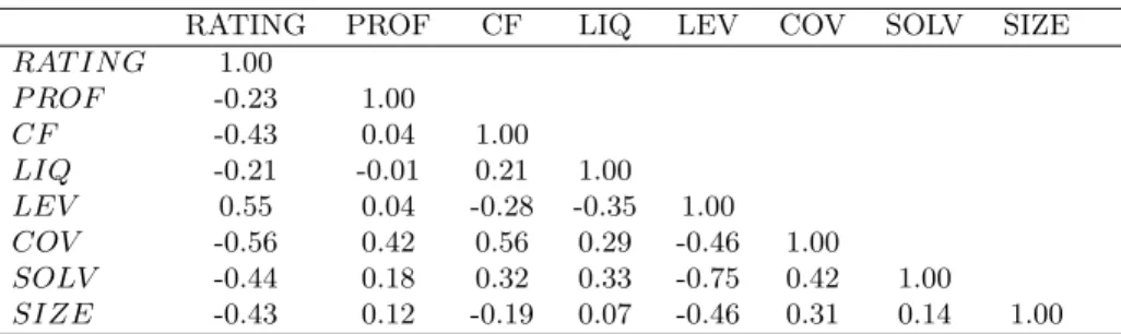
Table 2 provides a correlation matrix for the firm characteristics and the rating of the firm. It demonstrates that the characteristics have relatively low correlations with each other. In addition, the negative correlation between the credit ratings and profitability, cash flow, liquidity, coverage, solvency and size reflect the tendency for firms to obtain better ratings when they display healthy balance sheets. The opposite sign between credit ratings and leverage shows that highly indebted firms tend to attract worse ratings. This confirms that ratings are correlated with the indicators of creditworthiness on the balance sheet that investors expect ratings to measure.
Table 3 provides correlation information for lagged categories of ratings and initial ratings. There is some evidence that lagged ratings and initial ratings in the same category are positively correlated, presumably because there are firms that do not make transitions from their initial rating. Potentially the high correlation could result in multicolinearity in the equations where lagged and initial ratings are included together, therefore, in order to avoid drawing all our conclusions from models where this could be the case, we compare several different specifications in our results where lagged and initial ratings are included separately.
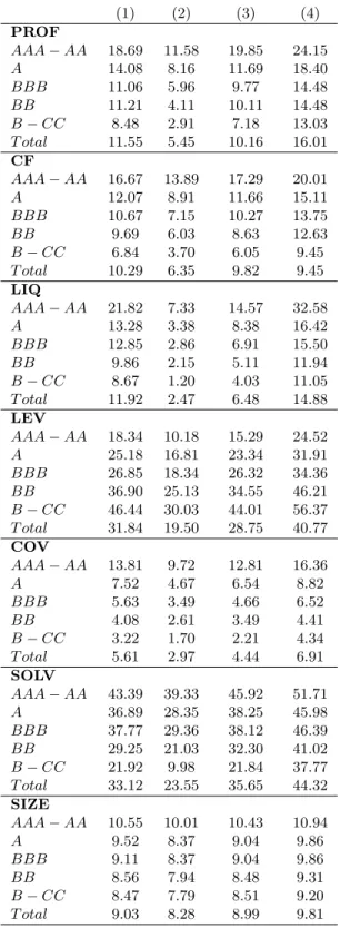
Table 4 reports summary statistics of our explanatory variables. We observe that firms belonging to the investment grade spectrum (BBB and above) have higher profit margins, higher cash flow
values, are more liquid, less leveraged, have higher coverage ratios, more solvent and larger compared to high yield firms (below BBB).
5
Results
In this section we report the estimation results.
5.1 The linear probit model
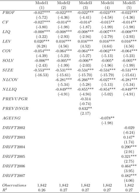
The first column of Table 5 reports our baseline model, which we refer to as model 1. We will later compare the performance of other models against this baseline. The result shows that, with the exception of the measure of leverage, an increase in all linear terms in the firm-specific variables improves the credit rating (they have significant negative coefficients which predicts a better rating category with a lower number). As profitability, cash flow, interest coverage, liquidity and solvency improve and as the firm has higher total sales so the firm receives a better predicted rating as expected. Leverage has a positive effect, worsening the credit rating as we might expect. Model 1 has an R2 of 0.26.
5.2 The non-linear probit model
Results for the nonlinear model (model 2) due to van Gestel et al. (2007) are presented in the second column of Table 5. The nonlinear terms apply the hyperbolic tangent transformation to variables to floor the impact of large negative or positive values of the variables on the predicted rating. We first check whether the non-linear terms are significant by determining whether the coefficients can be restricted to zero. The non-linear transformations of coverage (NLCOV) and liquidity (NLLIQ) reject this hypothesis with a p-value of 0.92 for joint hypothesis that the coefficients are zero. The nonlinear model has similar signs and significance of the linear terms for coverage and liquidity. Nonlinear terms are strongly significant and have negative coefficients, while linear terms retain their signs and significance. The effect of the nonlinear terms raises theR2 from 0.26 to 0.27. This indicates that minor improvement in the fit of the model is achieved with the addition of nonlinear terms, but the predictions of ratings reported later show a larger improvement.
5.3 Momentum, ageing and drift
Columns three through five in Table 5 offer an indication of the importance of momentum (model 3), ageing (model 4) and drift (model 5), described earlier in the paper. Carty & Fons (1993) were the first authors to note that a firm’s rating depended on whether the firm had previously been upgraded or downgraded. They concluded that firms that had been downgraded were more likely to see subsequent downgrades, while firms that had been upgraded were not more likely to be upgraded. The results in column 3 uphold these findings. The dummy variable indicating that firms have had a previous upgrade has a negatively signed coefficient, but it is not significantly different from zero, while a dummy variable indicating that firms that have had a previous downgrade has a positively signed coefficient, which is significant. There seems to be some evidence for momentum along the lines of Carty & Fons (1993) in our sample. There is also evidence of ageing. When we allow for the number of periods in the previous rating state, following a change in the rating state, we find that this variable has a negative and significant coefficient (reported in column four, Table 5). This means that the rating improves with the length of time in the previous rating state, which confirms evidence of ageing identified by Carty & Fons (1993), Lando & Skodeberg (2002) and Kavvathas (2001). Finally, we consider evidence of drift, which can be a result of variations in the standards of ratings agencies in assigning ratings or a variation in credit quality of firms seeking ratings over time, (see Blume et al. (1998), Cantor & Mann (2003) and Amato & Furfine (2004)). We report the coefficient on the difference in the percentage of firms experiencing an upgrade minus the percentage of firms experiencing a downgrade for each calendar year. We find that the estimated coefficients are significant for all but 2002, and all significant variables are positive and increasing in magnitude, implying that there is a tendency for ratings to worsen over time. This offers support for Blume et al. (1998) but it is not clear whether this is due to stricter ratings by agencies, or a deterioration in credit quality of firms being rated. Despite the strong evidence in favor of momentum, ageing and drift, we find that it adds almost nothing to the goodness of fit for these rating probit models.
5.4 Allowing for state dependence in ratings
Lando & Skodeberg (2002), Kavvathas (2001), Behar & Nagpal (1999) and Bangia et al. (2002) note that the rating transition is dependent on the previous rating category. We now introduce initial and lagged values of the rating for each firm in to allow for state dependence and initial conditions in results reported in Table 6. In columns one and two (models 6 and 7) we report the probit model when we allow for lagged and initial ratings separately and without other variables present, then in column three we report their impact when both lagged and initial ratings are included in the model, with no other variables in the equation (model 8). Then, in columns four, five and six, we report their impact with firm-specific variables included (models 9, 10 and 11). Finally, we report a model where we allow for the average of the past three years ratings instead of the rating in the previous period (model 12). This provides a range of results that allow us to determine the relative importance of lagged and initial rating data, which provide evidence for a type of momentum in models of ratings. All the models include some element of state dependence and it remains to be seen whether these models improve on the predictions of the models in Table 5.
The findings in these columns show that the previous or initial ratings are significant predictors of current rating in nearly every case. A positive and significant coefficient on the lagged rating (relative to the baseline rating of A) means that the firm with this rating in the previous period is predicted to have a rating this period with a higher ordinal value than A this period. (We recall that higher ordinal values are associated with lower ratings.) The opposite is true for negative coefficients. So firms with AAA-AA ratings in the previous period(s) are predicted to have ratings above A, and firms with BBB ratings or below in the previous period(s) are predicted to have ratings below A. Because these numbers are larger negative numbers for firms with AAA-AA ratings versus those with A ratings they will have correspondingly lower predicted ratings i.e. ratings that are higher on the rating scale.
We compare these models with two models that allow for state dependence in the rating - based on first lagged and initial ratings and an average of lagged ratings over the previous three years, and the initial rating. The estimates are similar to those reported in the previous columns in the following respects. We observe that linear and nonlinear variables retain their signs and significance
in most cases. The variables are not as strongly significant as they were in other models, which suggests that some of their significance in the previous model resulted from state dependence in the ratings, which is now measured directly by the lagged rating and the initial rating. Nevertheless the linear and nonlinear terms do not lose all their significance in every case, and we retain these variables in our model. We also find that the lagged dependent variables - included to formally test for state dependence - are highly statistically significant. Therefore we conclude that the previous state matters for the prediction of the rating today, and if a firm was rated below investment grade int−1 it is predicted to remain in the high-yield spectrum in the current period; similarly, being rated as investment grade in the previous period increases the probability of being rated as an investment grade issuer in the current year. As we will see later this prediction is almost always a correct prediction. When we consider the effect of the average rating in periods t−1, t−2 and t−3 in place of the lagged rating, we find a similar result.
The coefficients on lagged and average ratings show a similar gradient in the magnitude of the coefficient as one moves from a previous rating status of CC to AAA-AA. Embedding this state dependence through the previous rating or the average rating of the three previous years offers a substantial improvement in the fit of the model. So firms with AAA-AA ratings in the previous period(s) are predicted to have ratings above A, and firms with BBB ratings or below in the previous period(s) are predicted to have ratings below A. The estimated coefficients for the initial period observations are also highly significant. They show similar characteristics to the previous period rating for firms with initial ratings above A, since the coefficients are negative and larger negative numbers as the initial rating improves. Below A, firms with BB initial ratings and B-CC initial ratings have worse predicted ratings than those with an initial A rating, while BBB rated firms appear to have better predicted ratings.
Models with state dependence have higher R2 values than models without state dependence,
but we now compare the predictive performance in- and out-of-sample using root mean squared errors, Diebold Mariano statistics and in contingency tables.
6
Predictions
6.1 In-sample predictions
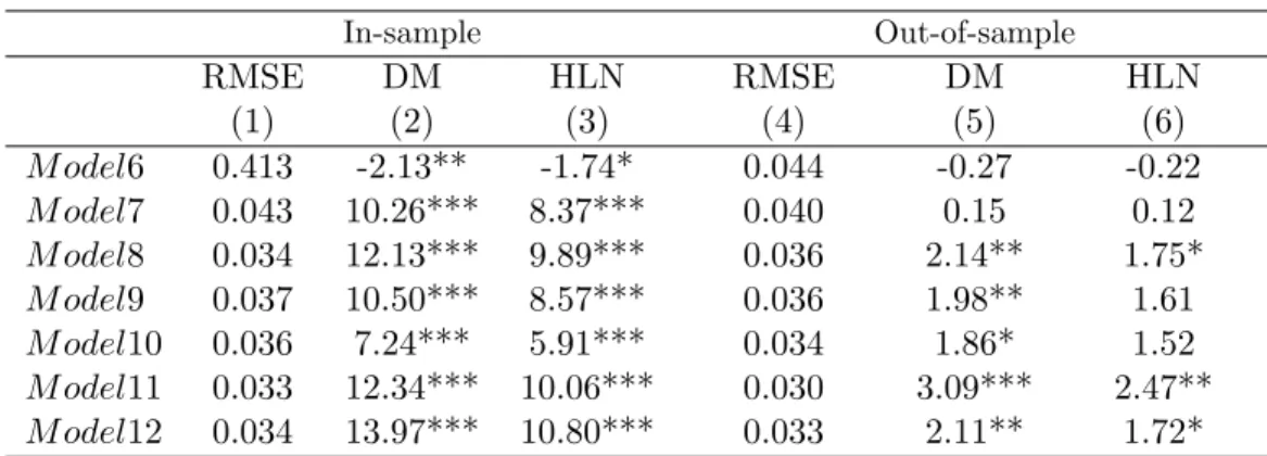
We begin by evaluating the forecasts for the models presented in Table 5. We report in Table 7, columns one to three, Root Mean Squared Errors (RMSE) as well as values for the Diebold-Mariano and the Harvey-Leybourne-Newbold statistics, compared to the baseline model (model 1) in Table 5. The results suggest that model 3 displays the smallest RMSE and there is evidence of a statistically significant difference between model 1, which is the baseline model, and models 2, 3 and 4 and 5. According to the DM and HLN tests, only models 2, 3 have superior predictive ability than the linear baseline model. In columns one through three of Table 8 we show RMSE and values for DM and HLN statistics for the models presented in Table 6. On the basis of the above mentioned statistics, there is significant difference in the performance of all models versus the baseline model. Thus all models (except model 6) reported in Table 6 perform better than the baseline model. The model with state dependence (model 11) displays the smallest RMSE and is significantly superior to the baseline model.
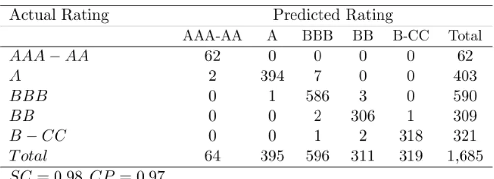
For the model with the smallest RMSE (model 11, with state dependence, shown in Table 6) we present a contingency table where one can compare predicted ratings to actual ratings. The outcome of this exercise is shown in Table 9. Reading across each row gives the number of predicted observations per category against the actual outcome in the leftmost column. For example, the first row shows the number of observations with actual rating of AAA-AA, while the second row shows those with rating A etc. To correctly evaluate the predictive ability of our model we employ two different statistics,SC andCP. The model correctly predicts AAA-AA 62 times, A 394 times, BBB 586 times, BB 306 times and B-CC 318 times. There are 949 occasions when the correct prediction is made, hence we find that the SC= 1666/1685, which suggests that we have approximately 98 percent correct predictions. The outcome of this exercise needs to account for the influence of the dominant outcome by reporting the Merton correct predictions statistic. This test calculates correct predictions using the proportion of correct predictions for each of the five rating categories. This test produces CP= 0.97 for the model with state dependence. Comparing this result with other authors’ results we find Blume et al. (1998) ordered probit model for bond issuers from
1978-SC=0.52 and CP=0.26 for the model of bond issuing forms for data from 1984-2001 with time dummies included. The main conclusion that can be drawn from this exercise is that credit ratings are indeed highly autocorrelated and previous years’ ratings are a key variable when predicting current ratings in-sample.
6.2 Out-of-sample predictions
This section presents out-of-sample predictions of ratings using the past and current information available up to time T. We use an expanding window method, which allows the successive obser-vations to be included in the initial sample prior to forecast of the next one-step ahead prediction of the rating while keeping the start date of the sample fixed. By this method, we forecast future ratings ˆqt+1, ˆqt+2 etc. The initial estimation window is 2000 to 2004 and the first prediction date
is year 2005. We then increase T by one each time until T reaches year 2007.
Columns four, five and six of Table 7 report RMSE and values for DM and HLN statistics for models in Table 5. We are able to reject the null hypothesis of equal forecasting performance in all four models. Specifically, models 2 and 3 are significantly better in terms of forecasting ratings than the baseline model. Table 8 reports the relative performance using RMSE, DM and HLN statistics comparing models with the baseline model for models in Table 6. We identify five out of seven cases where there is evidence of significant difference between the baseline model and the competing models. Once again the model with state dependence (model 11) displays the highest DM statistic value and the lowest RMSE.7
Table 10 illustrates the contingency table of the predicted against actual outcome out-of-sample results for the model with state dependence. As with the in-sample results, the predictive ability of the out-of-sample predictions is upheld when lagged values of ratings and initial ratings are included, since SC=0.94 per cent and the Merton correct prediction statistic indicates CP=0.93. The prediction out-of-sample is remarkably good, and shows that state dependence is a feature of ratings that helps forecasts.
7We have also tested the model with state dependence versus all other competing models. According to both DM and HLN statistics, the model with state dependence is significantly better in terms of forecasting ratings.
7
Conclusion
Many models of the relationship between credit ratings and a firm’s financial characteristics have used a linear probit model. In this paper we introduce nonlinear terms and allow ratings to vary due to ageing, momentum and drift. We then introduce state dependence in the form of lagged and initial ratings. The resulting model shows that non-linearities and state dependence terms improve the fit of a model seeking to determine a firm’s credit rating. When we analyze the ability of such a model to predict ratings we find that in-sample and out-of-sample the model with non-linearities and state dependence predicts much better than the baseline linear probit model. It appears that allowing for state dependence offers greater gains than allowing for non-linearities alone (although these offer some improvement in prediction) offering an SC score that is correct 98 percent of the time, and a CP score correct 97 percent of the time. The state-dependent model has the best performance evaluated by a Diebold-Mariano statistic. When we compare the performance of the model with state dependence out-of-sample we find that its performance does not deteriorate very much. It is correct on a SC basis 94 percent of the time, and on a CP basis 93 percent of the time out-of-sample, allowing for predictions one year ahead for three years 2005-2007; once again this model is superior according to the Diebold-Mariano statistic. We conclude that the use of information on the initial condition of the rating of the firm and the last observation of its actual rating helps the model correctly predict the rating more often than a model that excludes this information.
References
Altman, E. (1968). Financial ratios, discriminant analysis and the prediction of corporate bankruptcy. Journal of Finance,23, 189–209.
Amato, J. & Furfine, C. (2004). Are credit ratings procyclical? Journal of Banking and Finance,
28, 2641–2677.
Anderson, T. (1984).An introduction to multivariate statistical analysis. Wiley: New York. Bangia, A., Diebold, F., & Schuermann, T. (2002). Ratings migration and the business cycle, with
applications to credit portfolio stress testing.Journal of Banking and Finance,26, 445–474. Behar, R. & Nagpal, K. (1999). Dynamics of rating transition. Working paper, Standard and Poor’s. Blume, M., Lim, F., & MacKinlay, A. (1998). The declining credit quality of us corporate debt:
Myth or reality? Journal of Finance,53, 1389–1413.
Calomiris, C., Himmelberg, C., & Wachtel, P. (1995). Commercial paper, corporate finance, and the business cycle: A microeconomic perspective. Canergie-Rochester Conference Series on Public
Policy,42, 203–250.
Cantor, R. & Mann, C. (2003). Are corporate bond ratings procyclical? Special comment, Moody’s. Carty, L. & Fons, J. (1993). Measuring changes in corporate credit quality. Special report, Moody’s. Chava, S. & Jarrow, R. (2001). Bankruptcy prediction with industry effects. Working paper, Cornell
University.
Chortareas, G., Jiang, Y., & Nankervis, J. (2011). Forecasting exchange rate volatility using high-frequency data: Is the euro different? International Journal of Forecasting (forthcoming). Diebold, F. & Mariano, R. (1995). Comparing predictive accuracy. Journal of Business and
Eco-nomic Statistics,13, 253–263.
Duffie, D. & Singleton, K. (2003).Credit risk: Pricing, measurement and management. Princeton University Press: New Jersey.
Fitch (2006). Corporate rating methodology. Special criteria report, Fitch Ratings.
Frydman, H., Kallberg, J., & Kao, D. (1985). Testing the adequacy of Markov chain and mover-stayer models as representations of credit behavior.Operations Research,33, 1203–1214.
Frydman, H. & Schuermann, T. (2008). Credit rating dynamics and Markov mixture models.
Journal of Banking and Finance,32, 1062–1075.
Gonzalez, F., Haas, F., Johannes, R., Persson, M., Toledo, L., Violi, R., Wieland, M., & Zins, C. (2004). Market dynamics associated with credit ratings.Aliterature review. Occasional paper 16, European Central Bank.
Greene, W. & Hemsher, D. (2008). Modeling ordered choices: A primer and recent developments. Working paper 26, New York University, Leonard N. Stern School of Business, Department of Economics.
Harvey, D., Leybourne, S., & Newbold, P. (1997). Testing the equality of prediction mean squared errors. International Journal of Forecasting,13, 281–291.
Heckman, J. (1981). The incidental parameters problem and the problem of initial condition in esti-mating a discrete-time data stochastic process. In: Manski, C. & McFadden, D. (eds.),Structural Analysis of Discrete Data with Econometric Application, MIT Press: Cambridge.
Henriksson, R. & Merton, R. (1981). On market timing and investment performanceII.Statistical procedures for evaluating forecasting skills. Journal of Business,54, 513–553.
Horrigan, J. (1966). The determination of long-term credit standing with financial ratios. Journal of Accounting Research,4, 44–62.
Kao, C. & Wu, C. (1990). Two-step estimation of linear models with ordinal unobserved variables: The case of corporate bonds. Journal of Business and Economic Statistics,8, 317–325.
Kaplan, R. & Urwitz, G. (1979). Statistical models of credit ratings: A methodological enquiry.
Journal of Business,52, 231–261.
Kim, T., Mizen, P., & Chevapatrakul, T. (2008). Forecasting changes inUKinterest rates.Journal
of Forecasting,27, 53–74.
Koopman, S. & Lucas, A. (2005). Business and default cycles for credit risk. Journal of Applied Econometrics,20, 311–323.
Lando, D. (2004).Credit risk modeling: Theory and applications. Princeton University Press: New Jersey.
Lando, D. & Skodeberg, T. (2002). Analyzing ratings transitions and rating drift with continuous observations.Journal of Banking and Finance,26, 423–444.
Lennox, C. (1999). Identifying failing companies: A re-evaluation of the logit probit, and DA approaches. Journal of Economics and Business,51, 347–364.
Lo, A. (1986). Logit versus discriminant analysis: A specification test and application to corporate bankruptcies. Journal of Econometrics,31, 151–178.
Maddala, G. (1983). Limited-dependent and qualitative variables in econometrics, vol. 3. Econo-metric Society Monographs, Cambridge University Press.
Merton, R. (1981). On market timing and investment performance I. An equilibrium theory of value for market forecasts. Journal of Business,51, 363–406.
Nickell, P., Perraudin, W., & Varotto, S. (2000). Stability of rating transitions.Journal of Banking and Finance,24, 203–227.
Odders-White, E. & Ready, M. (2006). Credit ratings and stock liquidity. Review of Financial Studies,19, 119–157.
Pagratis, S. & Stringa, M. (2009). Modelling bank credit ratings: A reasoned, structured approach toMoody’s credit risk assessement.International Journal of Central Banking,5, 1–39.
Pesaran, M. & Timmermann, A. (1994). A generalization of the non-parametricHenriksson-Merton test of market timing. Economics Letters,44, 1–7.
Pinches, G. & Mingo, K. (1973). A multivariate analysis of industrial bond ratings. Journal of Finance,28, 1–18.
Pogue, T. & Soldofski, R. (1969). What is it in a bond rating.Journal of Financial and Quantitative Analysis,4, 201–228.
R¨osch, D. (2005). An empirical comparison of default risk forecasts from alternative credit rating philosophies. International Journal of Forecasting,21, 37–51.
Shumway, T. (2001). Forecasting bankruptcy more accurately: A simple hazard model.The Journal of Business,74, 101–124.
van Gestel, T., Martens, D., Baesens, B., Feremans, D., Huysmans, J., & Vanthienen, J. (2007). Forecasting and analyzing insurance companies’ ratings. International Journal of Forecasting,
23, 513–529.
Wooldridge, J. (2005). Simple solutions to the initial conditions problem in dynamic, nonlinear panel data models with unobserved heterogeneity.Journal of Applied Econometrics,20, 39–54.
Table 1: Ratings per year AAA AA A BBB BB B CCC Observations 2000 2 8 40 72 34 34 4 194 2001 2 7 51 85 40 37 4 226 2002 2 7 55 83 44 33 7 231 2003 2 7 53 83 46 45 7 243 2004 1 7 53 92 48 51 6 258 2005 1 7 54 88 47 46 6 249 2006 1 7 55 86 42 37 4 232 2007 1 7 42 80 42 37 3 212 Observations 12 57 403 669 343 320 41 1845
Notes: The table presents the distribution of firms’ ratings by year based on a panel of firms from 2000 through 2007.
Table 2: Correlation matrix for ratings and firm-specific creditworthiness indicators
RATING PROF CF LIQ LEV COV SOLV SIZE
RAT IN G 1.00 P ROF -0.23 1.00 CF -0.43 0.04 1.00 LIQ -0.21 -0.01 0.21 1.00 LEV 0.55 0.04 -0.28 -0.35 1.00 COV -0.56 0.42 0.56 0.29 -0.46 1.00 SOLV -0.44 0.18 0.32 0.33 -0.75 0.42 1.00 SIZE -0.43 0.12 -0.19 0.07 -0.46 0.31 0.14 1.00
Notes: The table presents correlations. PROF= Earnings before interest and taxes over total sales, CF= Funds from operations to total assets, LIQ= Cash from operations to total liabilities, COV= Operating profits to interest expenses, LEV= Total debt over total assets, SOLV= Common equity over total assets, SIZE= Log of real total sales.
Table 3: Correlation matrix for lagged and initial ratings
AAA−AA−1 A−1 BBB−1 BB−1 B−CC−1 AAA−AA(1) A(1) BBB(1) BB(1) B−CC(1) AAA−AA−1 1.00 A−1 -0.10 1.00 BBB−1 -0.14 -0.38 1.00 BB−1 -0.09 -0.25 -0.35 1.00 B−CC−1 -0.09 -0.25 -0.35 -0.24 1.00 AAA−AA(1) 0.85 -0.06 -0.11 -0.10 -0.10 1.00 A(1) -0.05 0.93 -0.36 -0.24 -0.24 -0.10 1.00 BBB(1) -0.13 -0.35 0.95 -0.34 -0.35 -0.15 -0.36 1.00 BB(1) -0.09 -0.22 -0.32 0.90 -0.23 -0.10 -0.24 -0.33 1.00 B−CC(1) -0.09 -0.25 -0.35 -0.15 0.90 -0.10 -0.24 -0.35 -0.23 1.00
Notes: The table presents correlations. The one period lags of the ratings are reported as AAA-AA 1 etc. The initial period observations are reported as AAA-AA(1) etc.