Short-term Determinants of Idiosyncratic Sovereign Risk Premium:
A Regime-Dependent Analysis for European Credit Default Swaps
Abstract
This study investigates the dynamics of the sovereign CDS term premium, i.e. difference between 10Y and 5Y CDS spreads. It can be regarded a forward-looking measure of idiosyncratic sovereign default risk as perceived by financial markets. For some European countries this premium featured distinct non stationary and heteroskedastic pattern during the last years. Using a Markov switching unobserved component model, we decompose the daily CDS term premium of five European countries into two unobserved components of statistically different nature and link them in a vector autoregression to various daily observed financial market variables. We find that such decomposition is vital for understanding the short-term dynamics of this premium. The strongest impacts can be attributed to CDS market liquidity, local stock returns, and overall risk aversion. By contrast, the impact of shocks from the sovereign bond market is rather muted. Therefore, the CDS market microstructure effect and investor sentiment play the main roles in sovereign risk evaluation in real time. Moreover, we also find that the CDS term premium response to shocks is regime-dependent and can be ten times stronger during periods of high volatility.
Keywords:Credit Default Swaps, Sovereign Risk, Term Premium, Markov Switching Model, State
Space Model.
1. Introduction
Tensions in the euro area sovereign debt market represent the most recent form of the global financial crisis. The succession of events following the beginning of the European sovereign debt crisis has clearly underscored that excessive systemic sovereign credit risk can lead to detrimental real macroeconomic effects and financial instability. Indeed, it is because of the risk of macroeconomic shocks and financial contagion that regulators and governments are currently so concerned about sovereign-specific credit risk. However, there is little theoretical and empirical basis on how to interpret the short-term dynamics of sovereign risk premia (i.e., compensation for sovereign risk as perceived in real time by financial markets), which have changed very abruptly in recent years. The use of sovereign CDS has increased dramatically during the last decade. They represent key instruments for credit risk transfer related to sovereign exposures. However, since the onset of the U.S. subprime crisis they have become very controversial and many commentators have blamed them for exacerbating the credit crunch by allowing excessive leverage and risk-taking by financial institutions and even market manipulation (see Calice et al., 2013, for a discussion). CDS spreads are deemed to be a more direct measure of credit risk than sovereign bond yields, since they are not distorted by other risks unrelated to defaults and market microstructure (Longstaff et al., 2005). In particular, as CDS contracts do not require up-front funding, CDS spreads are less distorted by liquidity dry-up during crisis periods (Chen et al., 2007).
Despite a sizeable literature on credit risk, empirical studies on CDS that involve modeling of the entire credit curve are still rare. A major reason for this is that data on sovereign CDS premia for a wider range of maturities have only recently become available. Indeed, although CDS contracts on some sovereign issuers are extensively traded, the market is still rather illiquid. Consequently, there is a paucity of empirical work regarding their CDS term structure, with studies focused mainly on U.S. synthetic corporate indices such as the CDX (see Longstaff et al., 2008; Calice et al., 2012). Pan and Singleton (2008) explores the nature of default arrival and recovery implicit in the term structure of the sovereign spreads of Korea, Mexico, and Turkey.
Specifically, we posit that the CDS term premium embeds the economy-wide forward-looking default risks. We measure this term premium as the difference between sovereign CDS spreads at 10-year and 5-year maturities. These two maturities are the most liquid segments of the sovereign CDS market. Therefore, to our knowledge this is the first study to explicitly analyze the sovereign CDS term premium (Calice et al., 2012, examine the U.S. corporate CDX term premium). In general, the evolution of the CDS term premium across time resembles the behavior of the yield curve and follows a mean-reverting process, despite short-term spikes during periods of financial turmoil. These spikes can be seen as regime changes (normal times vs. turmoil). Consequently, we assume that the term premium can be decomposed by means of the unobserved component model into two components. The first is a stationary component, which corresponds to the theoretical behavior of the CDS term premium and as such should be driven by fundamental forces (see also Garratt et al., 2006). The second component, which is modeled as a driftless random walk process, represents a seemingly unpredictable component in the term premium. Essentially, this component captures market uncertainty, which induces random walk behavior in the overall CDS term premium. The apparent heteroskedasticity will also be accounted for. We do this by means of a Markov-switching model that allows for two different volatility regimes for each CDS term premium subcomponent.
Our study focuses on five European sovereigns whose CDS term premia experienced notable swings during the global financial crisis period, which in turn resulted in nonstationary patterns and abrupt changes in their volatilities. This applies both to countries of the EMU periphery (we consider Italy, Spain, and Portugal) and to Central European countries (we consider the Czech Republic and Poland).1 Our central argument here is that the evolving pattern of the sovereign CDS term premium can provide the relevant authorities with more detailed information on financial market perceptions of the vulnerabilities in sovereign debt markets as well as on the sources of propagation of those vulnerabilities. A better and deeper understanding of these forces will in turn serve as a useful tool for the identification of systemic and contagion risks and will also potentially enable authorities to respond effectively in advance in order to mitigate shocks jeopardizing financial stability.
A number of important empirical results emerge from this analysis. First, we show that the decomposition of the CDS premium of a sovereign entity is relevant and major changes in the CDS term premium are driven by spikes in the nonstationary component. Second, decomposing the CDS term premium proves useful in understanding its short-term dynamics. Most selected financial market variables, observed at high frequency, significantly affect the dynamics of the nonstationary component, which is a seemingly unpredictable random walk. Third, the CDS term premium shows very pronounced regime-dependent behavior. In particular, the response of the CDS term premium to normalized shocks to some financial variables can be ten times stronger during periods of high volatility. All in all, our results show that CDS market microstructure effects (i.e., liquidity) and investor sentiment (as measured by stock market returns and the VIX) seem to play the main role in sovereign risk evaluation. The regime-dependent behavior suggests the existence of market overshooting during turmoil periods. These findings cast some doubt on whether short-term movements of the CDS credit curve should be interpreted in terms of changes in sovereign default risk rather than as a (sometimes exaggerated) response to other factors arguably disconnected from the actual risk of the sovereign concerned.
The remainder of the paper is organized as follows. Section 2 provides some theoretical considerations on the economic determinants of the sovereign CDS term premium and describes the data used in the analysis. Section 3 presents our methodology. Section 4 reports the results from the empirical analysis. Section 5 summarizes the results and makes concluding remarks.
2. CDS Term Premium
The CDS term premium is measured as the difference between spreads at 10-year and 5-year maturities and can be viewed as representing the default risk uncertainty over a 5-year time horizon. Therefore, the CDS term premium of a sovereign can be interpreted as a forward-looking measure of sovereign default risk as perceived by financial markets in real time. It also seems that this term premium tracks more closely the idiosyncratic part of sovereign credit risk, as it is arguably less prone to contagion than sovereign CDS/bonds of certain maturity. If the forces of international
1 Data availability and reliability constrain our sample to these five countries, whereas countries such as Ireland and
Hungary could be included as well, unlike Greece, whose sovereign CDS quotes were distorted and bear little economic significant in the face of the expected imminent credit event that was finally declared in March 2012.
contagion are in place there is in principle no reason to believe that they might have a differential impact on 5-year and 10-year maturities and affect the term premium.2
2.1 Economics of the CDS Term Premium
To motivate our empirical strategy and to guide our empirical tests, we begin with a brief discussion of the theoretical properties of the CDS term premium.3 We extend the canonical formulation of deriving forward rates from the term structure of default-free interest rates (e.g., Harrison and Kreps, 1979) to a country’s CDS term premium. Hence, the analysis that follows is in the spirit of deriving forward rates from the term structure of default-free interest rates.4
Consider a unit of time t that denotes quarters. Suppose that mt t,1 denotes a stochastic discount factor and t t,1 is an indicator function that takes the value of 1 if a country is solvent over the interval
t t, 1
and the value 0 otherwise. This can in practice (e.g., by rating agencies) be approximated by the marginal default probability (MDP) and the cumulative probability of default (CPD). Then, the premium paid on 10Y sovereign CDS solves (in a risk-free world with complete and arbitrage-free markets):
40 40 10 , , , , , 1 1 0 0 1 t t t t s t t s t t t s t t s t s t s t s s s CDS E m E m L
(1)where Lsis the loss in the event of default between s-1 and s. The right-hand side of the equation can be rewritten as the sum of two terms, A and B, where
20 , , , 1 1 0 1 t t t s t t s t s t s t s s A E m L
(2)
40 , , , 1 1 20 1 t t t s t t s t s t s t s s B E m L
(3)The previous two equations can be rewritten as follows: 20 5 , , 0 t t t t s t t s s A CDS E m
(4) 5 , 20 , 20 20 20 20, 20 20, 20 t t t t t t t t t s t t s BE m
CDS E m
(5)where A is the solution for 5Y CDS bought at time t=0 and CDSt520 in the term B is the forward CDS spread of 5Y CDS at time t=20 (i.e., after 5 years, that is, when a 5Y CDS contract priced in A matures). Combining (1) and (3) we obtain
2
This is evident from simple correlation measures, which are substantially higher for pairs of sovereign CDS at certain maturity (5 or 10 years) than between the corresponding CDS term premia. Similarly, it is relatively straightforward to extract a single informative factor from a sample of CDS quotes than from a sample of CDS term spreads. Therefore, looking at the spread at a particular maturity implies the basic identification strategy of isolating idiosyncratic from common factors. This challenge has recently been tackled by several papers aimed at examining contagion, especially in the European context. By contrast, analysis of the slope of the sovereign CDS credit curve has been largely ignored in the literature.
3 This is not intended as an exhaustive summary, but is simply meant to illustrate the economic foundations of the
CDS term premium and give a specific example of the mechanisms our model predicts.
20 5 10 , 20 , 20 20 20 20, 20 20, 20 0 10 5 20 , , 0 t t t t t t t t t t s t t s s t t t t t s t t s s E m CDS CDS E m CDS CDS E m
(6)A strong link can be seen between the sign of the CDS term premium CDSt10CDSt5 and the sign of
5 10
20
t t
CDS CDS , which is the difference between the forward 5-year CDS premium and the current 10-year CDS premium. Therefore, the CDS term premium is negative when a decrease is expected in the demand for default protection in the future. For example, if a country is currently facing a financial crisis but it is expected to be out of the crisis within 5 years the probability of imminent default (in 5 years from now) is higher than a default at a longer time horizon (after 5 years).
Therefore, the sign of the CDS term premium is strongly related to investors’ predictions about the timing of a country entering a crisis, which in turn determines the probability of default. Of course, this is in general dependent on the state (and evolution) of the fundamentals of the country. However, CDS spreads and the CDS term premium (the cost of external funding) are both subject to substantial short-term variation. Therefore, our objective is to explore empirically the factors driving these short-term dynamics of the sovereign CDS market, specifically, the market perception that a country might enter a crisis as tracked by the CDS term premium. Evidently, such short-term dynamics cannot reasonably be linked to changes in fundamentals, which evolve rather slowly. Therefore, we focus on financial market variables that feature similar short-term dynamics as the CDS term premium.
2.2 Data
Our study focuses on selected European countries whose CDS term premia experienced the most notable swings between positive and negative territory, which in turn resulted in nonstationary patterns and abrupt changes in volatility. As a rule-of-thumb we focus on those countries for which the CDS term premium amounted to at least 30–40 basis points (positive or negative) for a period in excess of a single trading day.5 This applies to two groups of EU sovereigns: (i) the EMU periphery (Spain, Portugal, and Ireland; Italy is excluded from the analysis due to data constraints), and (ii) the CEE countries (the Czech Republic and Poland; Hungary is also excluded due to data constraints). Our data sample spans from September 2007 (for some countries slightly later) to February 2012. Since our main empirical focus is on the short-term dynamics of the CDS term premium, we use daily market data.6 The main source of data is Bloomberg LP.
In Figure 1 we plot the 10Y and 5Y sovereign CDS spreads (upper panel) and the respective CDS term premium and CDS market liquidity (lower panel). Interestingly, we can see that whereas positive values of the CDS term premium correspond to an upward-sloping sovereign yield curve driven by a liquidity premium, sovereign financial distress results typically in a negative term premium (i.e., similar to the inversion of the yield curve).7 In terms of statistical properties, it is
5 On the contrary, we disregard smaller deviations, which in our view can be attributed primarily to market
microstructure factors.
6 With daily data we can explore the richness in the variation of the observations. Monthly frequency time series
would exhibit less volatile dynamic behavior since the short-term fluctuations would simply average out.
7 The EMU periphery exhibits positive values over the 2007–2008 period, then fluctuates considerably in 2009 and
2010, and then turns negative. Finally, the term premium for the CEE countries (the Czech Republic, Hungary, and Poland) clearly reveals the changing perception of the “safety” of that region. The premium is initially positive, then
apparent that the CDS term premium (lower panel) should be mean-reverting, as it is the difference between two series (10Y and 5Y CDS spreads) that are either both stationary or both nonstationary but cointegrated. However, as can be seen in the lower panel, the CDS term premium often evolves as a nonstationary process. This seems to be related not only to long memory, but also to structural changes in the process that we need to account for.8
As we are interested in the sources of the short-term dynamics, we collect several financial market variables which are observable at daily frequency. It is worth pointing out that while variables (i)–(v) denote a set of key domestic variables tracking developments in the sovereign CDS market itself (liquidity) as well as other markets (sovereign bond market, money market, banking CDS market, stock market), variables (vi) and (vii) identify two potentially relevant international variables:
(i) Sovereign CDS market liquidity calculated as the average of the bid-ask spread of 10Y and 5Y CDS.
(ii) The slope of the bond yield curve of each sovereign, which is calculated as the difference between the 10Y and the 5Y government bond yield (bid-close). This slope is the bond market counterpart of the CDS term premium.
(iii) The short-term interest rate is proxied by the 3M money market interest rate for each country (3M Euribor for the euro area countries). It tracks monetary policy as well as liquidity conditions in the money market.
(iv) The stock index return, calculated as the daily return (in percentage points) of the local major stock market index.
(v) The CDS term premium of the banking sector, which is computed as the difference between the 10Y and the 5Y CDS quotes (mid-price) of the two largest banks by assets in each country. This variable encompasses the potential transfer of credit risk between sovereign debt and the domestic banking sector.
(vi) International sovereign spillover/contagion, which is proxied by a common factor derived from the CDS term premia of other EU countries (i.e., for each of the five countries considered here a factor is derived by applying the principal factor method to the CDS term premia of the remaining available EU countries except the one analyzed). Following Longstaff et al. (2011), we use only the first factor, which accurately captures most of the variance.
(vii) Stock market volatility, as measured by the Chicago Board of Options Exchange S&P500 Volatility Index (VIX). This variable reflects the overall market sentiment or the degree of risk aversion, which can have disturbing effects on sovereign risk premia.
moves into negative territory for several months towards the end of 2008, and has been positive since then (turning negative in late 2011 for Hungary).
8
An alternative approach to dealing with long-memory and structural breaks with high-frequency financial series, specifically the euro OIS spread, is provided by Cassola and Morana (2012).
Figure 1: Sovereign 5Y and 10Y CDS Spreads (Upper Panel) and Sovereign Term Premium/Spread and CDS Market Liquidity (Lower Panel) Spain 0 100 200 300 400 500 600 5 .4 .2 0 0 4 5 .1 0 .2 0 0 4 5 .4 .2 0 0 5 5 .1 0 .2 0 0 5 5 .4 .2 0 0 6 5 .1 0 .2 0 0 6 5 .4 .2 0 0 7 5 .1 0 .2 0 0 7 5 .4 .2 0 0 8 5 .1 0 .2 0 0 8 5 .4 .2 0 0 9 5 .1 0 .2 0 0 9 5 .4 .2 0 1 0 5 .1 0 .2 0 1 0 5 .4 .2 0 1 1 5 .1 0 .2 0 1 1 10Y CDS 5Y CDS Portugal 0 200 400 600 800 1000 1200 1400 1600 1800 5 .4 .2 0 0 4 5 .1 0 .2 0 0 4 5 .4 .2 0 0 5 5 .1 0 .2 0 0 5 5 .4 .2 0 0 6 5 .1 0 .2 0 0 6 5 .4 .2 0 0 7 5 .1 0 .2 0 0 7 5 .4 .2 0 0 8 5 .1 0 .2 0 0 8 5 .4 .2 0 0 9 5 .1 0 .2 0 0 9 5 .4 .2 0 1 0 5 .1 0 .2 0 1 0 5 .4 .2 0 1 1 5 .1 0 .2 0 1 1 10Y CDS 5Y CDS Ireland 0 200 400 600 800 1000 1200 1400 1 2 .1 0 .2 0 0 7 1 2 .4 .2 0 0 8 1 2 .1 0 .2 0 0 8 1 2 .4 .2 0 0 9 1 2 .1 0 .2 0 0 9 1 2 .4 .2 0 1 0 1 2 .1 0 .2 0 1 0 1 2 .4 .2 0 1 1 1 2 .1 0 .2 0 1 1 10Y CDS 5Y CDS Czech Republic 0 100 200 300 400 500 600 700 2 2 .5 .2 0 0 6 2 2 .1 1 .2 0 0 6 2 2 .5 .2 0 0 7 2 2 .1 1 .2 0 0 7 2 2 .5 .2 0 0 8 2 2 .1 1 .2 0 0 8 2 2 .5 .2 0 0 9 2 2 .1 1 .2 0 0 9 2 2 .5 .2 0 1 0 2 2 .1 1 .2 0 1 0 2 2 .5 .2 0 1 1 2 2 .1 1 .2 0 1 1 10Y CDS 5Y CDS Poland 0 50 100 150 200 250 300 350 400 450 1 .4 .2 0 0 3 1 .1 0 .2 0 0 3 1 .4 .2 0 0 4 1 .1 0 .2 0 0 4 1 .4 .2 0 0 5 1 .1 0 .2 0 0 5 1 .4 .2 0 0 6 1 .1 0 .2 0 0 6 1 .4 .2 0 0 7 1 .1 0 .2 0 0 7 1 .4 .2 0 0 8 1 .1 0 .2 0 0 8 1 .4 .2 0 0 9 1 .1 0 .2 0 0 9 1 .4 .2 0 1 0 1 .1 0 .2 0 1 0 1 .4 .2 0 1 1 1 .1 0 .2 0 1 1 1 .4 .2 0 1 2 10Y CDS 5Y CDS Spain -60 -50 -40 -30 -20 -10 0 10 20 30 1 .9 .2 0 0 7 1 .3 .2 0 0 8 1 .9 .2 0 0 8 1 .3 .2 0 0 9 1 .9 .2 0 0 9 1 .3 .2 0 1 0 1 .9 .2 0 1 0 1 .3 .2 0 1 1 1 .9 .2 0 1 1 1 .3 .2 0 1 2
CDS term premium (10Y - 5Y) CDS Liquidity
Portugal -600 -500 -400 -300 -200 -100 0 100 200 1 .9 .2 0 0 7 1 .3 .2 0 0 8 1 .9 .2 0 0 8 1 .3 .2 0 0 9 1 .9 .2 0 0 9 1 .3 .2 0 1 0 1 .9 .2 0 1 0 1 .3 .2 0 1 1 1 .9 .2 0 1 1 1 .3 .2 0 1 2
CDS term premium (10Y - 5Y) CDS Liquidity
Ireland -350 -300 -250 -200 -150 -100 -50 0 50 100 150 1 2 .1 0 .2 0 0 7 1 2 .4 .2 0 0 8 1 2 .1 0 .2 0 0 8 1 2 .4 .2 0 0 9 1 2 .1 0 .2 0 0 9 1 2 .4 .2 0 1 0 1 2 .1 0 .2 0 1 0 1 2 .4 .2 0 1 1 1 2 .1 0 .2 0 1 1
CDS term premium (10Y - 5Y) CDS Liquidity
Czech Republic -100 -80 -60 -40 -20 0 20 40 60 1 .9 .2 0 0 7 1 .3 .2 0 0 8 1 .9 .2 0 0 8 1 .3 .2 0 0 9 1 .9 .2 0 0 9 1 .3 .2 0 1 0 1 .9 .2 0 1 0 1 .3 .2 0 1 1 1 .9 .2 0 1 1 1 .3 .2 0 1 2
CDS term premium (10Y - 5Y) CDS Liquidity
Poland -40 -30 -20 -10 0 10 20 30 40 50 60 1 .9 .2 0 0 7 1 .3 .2 0 0 8 1 .9 .2 0 0 8 1 .3 .2 0 0 9 1 .9 .2 0 0 9 1 .3 .2 0 1 0 1 .9 .2 0 1 0 1 .3 .2 0 1 1 1 .9 .2 0 1 1 1 .3 .2 0 1 2
CDS term premium (10Y - 5Y) CDS Liquidity
Note: 10Y CDS is the sovereign 10Y CDS spread (mid-price), 5Y CDS is the sovereign 5Y CDS spread (mid-price), CDS term premium is the difference between 10Y CDS and 5Y CDS, and CDS liquidity is the average of the bid-ask spread of 10Y and 5Y CDS.
3. Methodology
We investigate the dynamic behavior of the sovereign CDS term premia of a selected group of European countries. Whereas economic logic suggests that these univariate series should be mean-reverting, for these sovereigns they have been characterized by pronounced nonstationary features during the recent eurozone sovereign debt crisis. Hence, to better understand the dynamics of the CDS term premium, it is crucial to address the nonstationarity methodologically. For this purpose, we decompose such series into a stationary component and a nonstationary component and study them separately. This provides a fairly robust statistical framework akin to the cycle-trend decomposition commonly used in business cycle analysis. Furthermore, our approach is strongly inspired by recent developments in inflation modeling. Whereas inflation (like the CDS term premium) is generally regarded from the theoretical viewpoint as being a mean-reverting process, empirical applications have started to explicitly account for its nonstationarity. Indeed, authors such as Stock and Watson (2007) have stressed the importance of distinguishing between stationary and nonstationary components and their different drivers. Whereas the nonstationary component of inflation is now believed to be driven by structural factors that are subject to regime changes (e.g., the monetary policy framework and the credibility of the inflation target), its stationary part can reasonably be linked to cyclical fluctuations of the economy in the original logic of the Phillips curve.
Several approaches to decomposing univariate time series have been proposed in the econometric literature. A well-established methodology is the unobserved components approach, postulated in separate contributions by Harvey (1985), Watson (1986), and Clark (1987). The econometric methodology employed in this paper relies upon the statistical approach developed initially by Nerlove, Grether, and Carvalho (1979) and extended by Harvey (1989) and Harvey and Shephard (1993). The essential element of this methodology is to estimate a model which considers the observed time series as being the sum of a permanent (nonstationary) and a transitory (stationary) component. These components capture salient features of the series that may be unobserved and are useful in explaining and predicting its time evolution. In terms of our decomposition of the CDS term premium, the stationary (mean-reverting) component underscores the fundamental driving forces in the economy, while the nonstationary (random walk) component captures the overall uncertainty underpinning the evolution of the fundamentals, which can be driven by financial shocks.9
As evidenced by the sharp increase in sovereign risk premia and their volatilities during the recent financial crisis, sovereign risk premia behave differently in distinct regimes. We assume that those changes are recurrent. By allowing for endogenous regime switches in volatility, one does not have to explicitly set a switching threshold value, but the data endogenously identify the switching to a different regime. Markov-switching (as opposed to models assuming smooth
9 Use of the terms “permanent” and “transitory” would be slightly confusing in our case. Whereas in business
cycle analysis, the GDP series have a permanent (nonstationary) trend and there is some temporary (stationary) cyclical fluctuation around the trend, in our case the CDS term premium should be a mean-reverting variable. Therefore, the fundamental part is mean-reverting and stationary as well, while the short-term spikes are nonstationary. Therefore, the economic meaning of the two components is different.
transition10) is motivated by the abrupt regime changes attributable to the high-frequency nature of the data. By adding Markov-switching disturbance terms into the two unobserved components, one can explicitly model high- and low-volatility regimes over different time periods. Although it complicates the estimation procedures – since additional filters must be employed to make inference on the hidden Markov chain process – allowing the two components to depend on different states of the economy provides an alternative approach to dealing with the potential heteroskedastic variance in the daily risk premia series.11 We assume that allowing for switches in disturbances represents a reasonable grade of approximation as opposed to allowing for switches in both coefficient and disturbances. The latter would potentially lead to a higher number of regimes, which would not be feasible for further empirical analysis.
3.1 Modeling the Unobserved Factors that Drive the Term Premia
Let X1,t represent the stationary component (STAT) that drives the term premium, and assume that X1,t is an Ornstein-Uhlenbeck process whose dynamic evolution can be described by the stochastic differential equation
1, 1 1, 1 1, k t k t t t t X e e X Z (7) where 1 250 t is the sampling interval and 1 1
1 2 k t e k
. It is easy to see that k0
implies e k t 1 and hence stationarity, k0 or t 0 implies e k t1, and the model converges to a unit root model.
Now, let X2,t be the second component that drives the term premium. We assume that it follows a driftless random walk (RW) process as shown in Eq. (8):
2,t 2 2,t
dX dZ (8)
where
2 is the scaled volatility parameter and dZ2,t is the standard Brownian motion, which can be assumed to be either dependent on or independent of dZ1,t.The discrete time version of Eq. (8) yields2,t 2, 1t 2 2,t
X X
Z (9)Although an RW process, such as the one described in (9), has infinite unconditional mean and variance, the conditional mean and variance can be measured as
10 Prominent examples of such models are time-varying parameter vector autoregression (TVP-VAR) and the
smooth transition autoregressive model (STAR).
11
The more conventional way of testing for financial time series heteroskedasticity is to consider ARCH-type volatility models, which allow constant unconditional volatility but time-varying conditional volatility. However, neglecting possible regime shifts in the unconditional variance, as shown in Lamoureux and Lastrapes (1990), would overestimate the persistence of the variance of a time series.
2, 2, 1 2 2, 2 t t t t t E X X Var X
(10)where the conditional expectation of the process at the current time t depends only on the
observation in the previous time period.
Given the two unobserved components constructed using Eq. (8) through Eq. (10), we estimate the parameter space as given by this system, with the dynamics of the two components updating in a Bayesian manner, namely, the Kalman filter algorithm based on a state space system. State space representation is usually applied in dynamic time series models that involve unobserved variables (e.g., Engle and Watson, 1981; Hamilton, 1994; Kim and Nelson, 1989). A typical state space model consists of two equations. One is a state equation that describes the dynamics of the unobserved variables, and the other one is a measurement equation that describes the relation between the measured variables and the unobserved state variables,
1 , ~ 0, t t t t X C FX Q (11) where 1, 2, t t t X X X ,
1
0 k t e C , 0 0 1 k t e F , 1, 2, t t t and 2 1 1 2 12 2 2 1 21 2 Q t .Rewritten in compact form, this expression reduces further to give
t t
Y HX (12)
where Yt is the term premium series and H
1 1 represents the weights of the two components in the term premium.3.2 Markov-Switching Disturbances
An additional feature of our model is that it allows each component’s disturbance term to depend on different states of the economy. In practice, we let the volatilities of the disturbance terms switch between high- and low-volatility regimes. Formally, we assume that 2
1
and 2 2
in Eq. (13) are driven by two discrete-valued, independent unobserved first-order Markov chain processes S1,t
0,1 and S2,t
0,1 given by
2 2 2 2 2 1 1, 1 1, 1 1 1 2 2 2 2 2 2 2, 2 2, 2 2 2 1 , 1 , t H t L H L t H t L H L S S S S (14)When both S1,t and S2,t are zero, the two components will be in the high-volatility state, as
2 2
1 1H
and 2 2
2 2H
; similarly, if both S1,t and S2,t equal 1, the two components will be in the low-volatility state, since 2 2
1 1L
and 2 2
2 2L
However, it is also possible for one component to be in the high-volatility state while the other is in the low-volatility state. The likelihood of the process remaining at the previous value or changing to the alternative depends on the probabilities of transition from one state to the other, which are shown below as
1,00 1, 1, 1 1,11 1, 1, 1 2,00 2, 2, 1 2,11 2, 2, 1 Pr 0 | 0 Pr 1 | 1 Pr 0 | 0 Pr 1 | 1 t t t t t t t t p S S p S S p S S p S S (15)
To estimate the transition probabilities as shown above, we need to choose the appropriate functional forms of the probability functions that govern the Markov chain variables. Since the transition probabilities have to be bounded within
0,1 the usual choice is to adopt the logistic transformation on the probability terms as
1,0 1,00 1, 1, 1 1,01 1,00 1,0 1,1 1,11 1, 1, 1 1,10 1,11 1,1 2,0 2,00 2, 2, 1 2,01 2,00 2,0 2,11 2, 2, 1 exp Pr 0 | 0 , 1 1 exp exp Pr 1 | 1 , 1 1 exp exp Pr 0 | 0 , 1 1 exp Pr 1 | 1 t t t t t t t t d p S S p p d d p S S p p d d p S S p p d p S S
2,1 2,10 2,11 2,1 exp , 1 1 exp d p p d (16)where d1,0,d1,1,d2,0, and d2,1 are the unconstrained parameters.
To estimate the state space Markov-switching model described previously, we use Kim’s filter (Kim, 1994), which is a numerical algorithm that combines the Kalman filter in estimating state space models and the Hamilton filter (Hamilton, 1989) in estimating Markov-switching models. Specifically, we use the estimation procedures developed in Calice et al. (2012).
3.3 VAR Analysis
Once we decompose the CDS term premia into the unobserved STAT and RW components, we can test for the impact of observed economic and financial variables on these components within a VAR setting. In particular, we assume that this propagation can be nonlinear depending on the volatility regime of each component. Therefore, central to our analysis is (i) whether the observed economic and financial variables have a different impact on STAT and RW and (ii) whether the impacts on STAT and RW differ in the low- and high-volatility regime. Therefore, we run (for each unobserved component of the CDS term premium STAT and RW) a standard VAR on subsamples defined by transition probabilities estimated as described above. Specifically, we use the probability of being in the high-volatility regime with a cutting value of 0.5, i.e., at lower probability values the component is in the low-volatility regime, and otherwise it is in the
high-volatility regime. Therefore, we keep observations from the high- and low-high-volatility regimes apart.12 The resulting four VAR(p) models can be written as follows:
0 0,5 p t t i t i STATt t Y c
Y I p
(17)
0 0,5 p t t i t i STATt t Y c
Y I p
(18)
0 0,5 p t t i t i RWt t Y c
Y I p
(19)
0 0,5 p t t i t i RWt t Y c
Y I p
(20)where Yt is the vector of p endogenous variables including the stationary component (STAT) or
the random walk (RW) component as well as six financial variables (defined below) observed at daily frequency. I is an indicator function that takes the value 1 when the estimated transition probability of being in the high-volatility regime st exceeds 0.5, and 0 otherwise. As we impose two independent first-order Markov chain processes, we attempt to capture the differential effect of each volatility regime on each subcomponent. Thus, we compute the generalized impulse response functions that are invariant to any ordering specification to trace out the responsiveness of the dependent variables (STAT or RW) to one unit generalized shock to each of the variables. It will be noted that the first step (the decomposition of the CDS premium into the two components and the estimation of the volatility regime for each of them) is subject to uncertainty, which also conditions the results obtained in the second step (VAR analysis). Unfortunately, as joint estimation in one step is empirically unfeasible, the uncertainty cannot be completely avoided. Still, we assume that this uncertainty does not significantly affect our results. In addition, we take a number of steps to reduce it. First, while the two estimated components are unobserved variables, they are (by construction) normally distributed and, therefore, the means of the impulse responses produced by the VAR are not affected. Besides the VAR analysis based on the STAT and RW subcomponents, we also consider as a robustness check the whole CDS term premium (without decomposition). Second, the estimation error of the unobserved component model is expected to be heteroskedastic, as more volatile periods are subject to higher uncertainty. That is why we explicitly allow for endogenous regime switches in volatility by adding Markov-switching disturbance terms into the two unobserved components. Consequently, in the VAR model we allow for subsample analysis keeping the observations from low- and high-volatility periods apart. However, there is also uncertainty associated with the very estimates of the switching probabilities. Therefore, we adopt a simplification consisting in using moving averages of the estimated switching probabilities, which avoids using the exact value estimated for each point in time and instead relies on their smoothed average on a window of one month. By doing
12 We believe that our two-step approach consisting in (i) univariate series decomposition and regime
identification and (ii) subsample analysis with standard linear VAR has some clear advantages over the use of more complicated VAR models such as threshold or Markov-switching VARs. Notably, it is very difficult to make inference on either, as a shock to an endogenous variable can imply a change of regime, which complicates the construction of the impulse response functions, as these depend on the sign and size of the shock. Threshold VAR additionally requires prior identification of the endogenous threshold variable, i.e., an assumption of what the threshold variable is. We do not possess such prior knowledge and simply assume that the regimes can be derived from the CDS term premium or its components. Moreover, we do not assume there are regimes that differ from those identified in the first step of the estimation procedure.
so, we also eliminate some erratic developments that would imply implausibly frequent regime switches. Finally, we perform a robustness check with alternative values of the switching probability to split the sample into low- and high-volatility regimes.13
4. Empirical Results
Using the methodology described in Section 3, we estimate for each country a series of nested Markov-switching unobserved component models. Furthermore, we run a battery of tests on the model specification to determine the preferred model to use in the empirical analysis.
4.1 Model Selection Tests
It is well known that for Markov-switching models the standard likelihood ratio test of the null hypothesis of linearity does not have the usual 2 distribution. The reason is that there are nuisance parameters which cannot be identified under the null hypothesis. As a result, the scores evaluated at the null hypothesis are identically zero.14 We use the Hansen (1992) procedure, which provides an upper bound on the pvalue for linearity, to determine the significance of the improvement for allowing Markov-switching disturbance terms in the two components. In addition, we consider more conventional ways of selecting models based on the Akaike Information Criterion (AIC) and Schwarz Bayesian Information Criterion (BIC). Finally, we verify our model selection results by running a series of residual diagnostic tests to establish whether the selected model is able to infer serial correlation and heteroskedasticity in the data series.
To implement the Hansen (1992) procedure, we need to evaluate the constrained likelihood under the null hypothesis over a grid of values for the nuisance parameters. Defining the restricted model under the null hypothesis of no regime switching of the two components’ disturbance terms as described in Eq. (12) with
12
210, and the alternative model under the assumption of Markov-switching disturbance terms (as shown in Eq. 16–18), the nuisance parameters are denoted as
1H, 2H,p1,00,p1,11,p2,00,p2,11
.Further, we test whether a model allowing correlated disturbance terms performs better than a model with restrictions to zero correlations. The results suggest that the models with correlated disturbance terms generally produce higher likelihood values and lower AIC and BIC statistics. We verify this result with the residual diagnostic tests, where we test the overall randomness of the residuals of the models (the summation of the disturbance terms of the two components) with the null hypothesis of assuming randomness. It is important to stress that although the most flexible model is not a powerful autocorrelation measure in the residuals (like all the other
13 Threshold VAR (e.g., Balke, 2000) allows estimation of the unknown threshold (for a selected threshold
variable, which in our case is the estimated probability of the high-volatility regime) as well as inference of its relevance, rather than assuming that the threshold is equal to a certain value (in our case 0.5). However, our use of the moving average of the estimated probabilities makes the identification of the regime “rougher,” which in our view avoids the need for a very precise threshold estimation method.
alternative models) it nonetheless does a relatively good job in capturing the ARCH effects in the residuals.15
4.2 Estimation of the Markov-Switching Unobserved Component Model
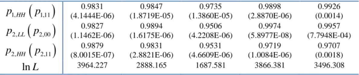
Table 1 reports the maximum likelihood estimates from the most flexible and best performing model for the five countries (Spain, Portugal, Ireland, the Czech Republic, and Poland). As is evident, there is a significant regime-dependent long-term equilibrium of the stationary component for Spain, Portugal, Poland, and Ireland, but not for the Czech Republic. The two regimes, which are defined in our model as low- and high-volatility regimes of the term premium series, are strongly associated, respectively, with a positive and negative long-term equilibrium level of the stationary component for all countries with the exception of Poland.
In normal market conditions, the CDS term premium is generally upward sloping, which suggests that the market is not factoring in imminent default risks but expectations about protection costs are increasing with the tenor of the CDS contract. On the contrary, the term premium could turn negative if market conditions worsened in the immediate future. Since a negative long-term equilibrium level of the term premium is in general interpreted as the result of a short-term deterioration in credit markets, the coincidence of this with high-volatility regimes of the term premium is not a surprise. In other words, a worsening of credit market conditions brings about a surge in volatility as well as an automatic correction of the term premium to its long-term equilibrium.
Table 1: Estimation Results
Parameters Spain Portugal Ireland Czech Republic Poland L
0.0485 (3.1056E-05) 0.0197 (1.0804E-05) -0.0475 (1.4887E-05) 0.0225 (5.8769E-05) 0.1433 (0.0312) H -0.0190 (2.1885E-05) -3.0668 (1.2516E-04) -1.4020 (0.2443) -0.0105 (0.1668) 0.3477 (0.0227) L k 22.4741 (0.0012) 66.2939 (0.0014) 126.4403 (8.5057E-03) 0.1425 (1.5520E-03) 0.4226 (0.1297) H k 0.6438 (4.9187E-05) 0.6822 (1.9017E-04) 0.4118 (0.0324) 0.0783 (0.7619) 0.3477 (0.0227) 1,L 0.0320 (1.0230E-05) 0.2502 (1.7560E-05) 0.0378 (1.7379E-05) 0.0763 (8.5528E-07) 0.0010 (2.0738E-03) 1,H 0.5147 (1.9946E-05) 1.6820 (9.9406E-05) 0.5189 (0.0002) 0.4892 (2.2147E-05) 0.0109 (0.0522) 2,L 0.0315 (1.2994E-05) 0.0221 (7.6557E-06) 0.0711 (1.1732E-05) 0.1033 (1.3741E-07) 0.2457 (3.8638E-03) 2,H 0.5534 (6.8113E-05) 3.2845 (3.5630E-06) 0.7310 (6.7586E-06) 0.7047 (2.6688E-06) 0.8019 (0.0100) 1 ,2L L 0.6073 (3.2774E-04) 0.6317 (9.2002E-04) 0.6300 (4.8726E-04) -0.0839 (1.4499E-03) -0.8520 (1.6914) 1H,2L 0.8248 (4.0280E-04) 0.8010 (5.0474E-05) 0.7360 (0.3688) 0.1917 (4.0405E-04) -0.8043 (1.2358) 1 ,2L H 0.7743 (8.3614E-05) 0.8228 (6.6015E-04) -0.7710 (0.5146) 0.9897 (0.3076) -0.9964 (0.2025) 1H,2H 0.7472 (1.6348E-04) 0.7882 (1.0329E-04) -0.8316 (2.1876E-04) -0.3593 (9.6442E-04) 0.8811 (0.4177) 1,LLp
p1,00 (9.0534E-07) 0.9863 (1.8354E-06) 0.9712 (4.8348E-06) 0.9430 (1.0508E-06) 0.9626 (1.7403E-03) 0.9682
1,HH
p
p1,11 (4.1444E-06) 0.9831 (1.8719E-05) 0.9847 (1.3860E-05) 0.9735 (2.8870E-06) 0.9898 (0.0014) 0.9926 2,LLp
p2,00
(1.1462E-06) 0.9827 (1.6175E-06) 0.9894 (4.2208E-06) 0.9506 (5.8977E-08) 0.9974 (7.7948E-04) 0.9957 2,HHp
p2,11
(8.0015E-07) 0.9879 (2.8821E-06) 0.9831 (4.6609E-06) 0.9531 (1.0084E-06) 0.9719 (0.0018) 0.9707 lnL 3964.227 2888.165 1687.581 3866.381 3496.308Note: The standard errors of the estimates are in parentheses.
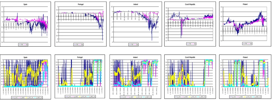
Figure 2 provides the decomposition of the CDS term premium into the STAT and RW components (upper panels) as well as the estimated probabilities of each component switching to the high-volatility regime (lower panels). First of all, we note that the two components show rather dissimilar behavior and most of the spikes in the term premium are driven by the RW component and can be interpreted as departure from the mean-reverting behavior of the STAT component, whereas the mean reversion is the expected behavior of the whole CDS term premium/spread. Therefore, we interpret the STAT component as the fundamental part of the CDS term premium, whereas the RW component is the random part whose nonstationarity is driven by shocks.
Following this logic, the most interesting periods are those when the STAT component turns negative, i.e., when the financial markets expect an immediate possibility of sovereign default and this cannot be interpreted as random behavior. This happens for Spain, Portugal, and Ireland following the markets’ reactions to the European sovereign debt crisis, when banks’ asset write-downs and diminishing liquidity in funding markets raised the degree of uncertainty about future credit events. For Spain, worries about the government’s ability to repay its debt, as well as the negative state of the economy,16 further intensified the strains in financial markets. For Portugal, the cut of its sovereign bond rating by Moody’s by two notches seems to be the key determinant of the steady decline of its term premium in the latter part of the sample period, with STAT reverting to negative territory in summer 2011, when the crisis intensified. As in the case of Portugal, the market’s concerns over Ireland’s debt spiral intensified when Moody’s downgraded Irish sovereign bonds to junk status, which drove STAT to negative territory in very early 2011. Whereas the STAT of these countries returned to zero afterwards, the CDS term premia remained in negative territory due to a very negative RW component. Indeed, the volatile RW component is the main driver of the significant departures of the term premium into negative values and thus its overall nonstationarity.
The Central European countries exhibit different decomposition results from Ireland and Portugal. The term premium series for these two countries is positive for most of the sample period, with the notable exception of 2008. For most of the 2009–2010 period, both the RW and stationary components for the Czech and Polish term premia experience a relatively “mild” regime. This could possibly be explained by improving conditions in credit markets and a better outlook for the CE region. Although both countries’ banks belong to global financial groups that have been severely hit by the “credit crunch,” their activities are mainly inward oriented. The tendency to
16
As Spain is one of the largest eurozone economies (larger than Greece, Portugal, and Ireland combined) the condition of its economy is of particular concern to international observers. Under pressure from the United States, the IMF, other European countries, and the European Commission, the Spanish government eventually succeeded in trimming the deficit from 11.2% of GDP in 2009 to an expected 5.4% in 2012.
generate profits mainly through dynamically expanding retail banking activities has ensured a high level of balance sheet liquidity for Czech and Polish banks and has avoided a strong dependence on funds from foreign markets, unlike in Spain, Portugal, and Ireland.
The estimation results also reveal that for all these countries the mean reversion speed has an inverse relationship with the volatilities, i.e., a high speed of mean reversion materializes when the term premium is in a relative stationary state, whilst it takes longer for the term premium to revert to its long-term mean when the market enters the high-volatility regime. During non-crisis periods, asset prices are less likely to stay high or low period-to-period, but mean revert quickly to their long-term equilibrium values. In other words, mean-reverting asset prices imply a low probability of ending up in the tail of the distribution.17 Portugal and Ireland show similar inverse relationships between the mean-reverting speed parameter and the volatility regimes.18
As for the Czech Republic and Poland, the rising profile of the term premium generates considerable volatilities in the market. The transition probabilities, plotted in Figure 4, clearly show that the term premium enters the high-volatility regime in early 2011 for both countries.19 Although the Czech Republic and Poland have more favorable credit market conditions than Portugal and Ireland, the spikes in the transition probabilities of both components switching to the high-volatility regime after mid-2011 may be an indication of potential spillover effects, as volatility shocks quickly transmitted to the Central European countries’ capital markets.
Given the lead of the RW component, especially in its high-volatility regime, it seems interesting to test whether their movements are merely random or whether they can be attributed to some other observable market developments. This is the subject of the following analysis, which looks at the potential determinants of each component in each regime separately.
17 Our estimate of the Spanish mean-reverting speed (k) is 22.4741 in the low-volatility regime, which
translates into a first-order autocorrelation of -0.9140. The speed in the high-volatility regime, on the other hand, falls to 0.6438 or -0.9974 in terms of first-order autocorrelation, revealing very persistent behavior of the stationary component in the high-volatility regime but less persistent behavior in the low-volatility regime.
18 Our estimate of the mean-reverting speed is 66.2939 (126.4403)in the low-volatility regime, which translates
into a first-order autocorrelation of -0.7671 (-0.6030) for Portugal (Ireland). The speed in the high-volatility regime, on the other hand, falls to 0.6822 (0.4118) or -0.9972 (-0.9983) in terms of first-order autocorrelation, which suggests very persistent behavior of the stationary component in the high-volatility regime.
19 Particularly for Poland, the estimate of the high-volatility regime long-term equilibrium (0.3477) is much
Figure 2: CDS Term Premium Decomposition (Upper Panel) and Probabilities of Switching to High-Volatility Regime (Lower Panel)
Spain -0.4 -0.3 -0.2 -0.1 0 0.1 0.2 0.3 1 .9 .2 0 0 7 1 .1 2 .2 0 0 7 1 .3 .2 0 0 8 1 .6 .2 0 0 8 1 .9 .2 0 0 8 1 .1 2 .2 0 0 8 1 .3 .2 0 0 9 1 .6 .2 0 0 9 1 .9 .2 0 0 9 1 .1 2 .2 0 0 9 1 .3 .2 0 1 0 1 .6 .2 0 1 0 1 .9 .2 0 1 0 1 .1 2 .2 0 1 0 1 .3 .2 0 1 1 1 .6 .2 0 1 1 1 .9 .2 0 1 1 1 .1 2 .2 0 1 1 1 .3 .2 0 1 2 RW Stat Portugal -4.5 -4 -3.5 -3 -2.5 -2 -1.5 -1 -0.5 0 0.5 1 1 .9 .2 0 0 7 1 .1 2 .2 0 0 7 1 .3 .2 0 0 8 1 .6 .2 0 0 8 1 .9 .2 0 0 8 1 .1 2 .2 0 0 8 1 .3 .2 0 0 9 1 .6 .2 0 0 9 1 .9 .2 0 0 9 1 .1 2 .2 0 0 9 1 .3 .2 0 1 0 1 .6 .2 0 1 0 1 .9 .2 0 1 0 1 .1 2 .2 0 1 0 1 .3 .2 0 1 1 1 .6 .2 0 1 1 1 .9 .2 0 1 1 1 .1 2 .2 0 1 1 1 .3 .2 0 1 2 RW Stat Ireland -3 -2.5 -2 -1.5 -1 -0.5 0 0.5 2 9 .1 .2 0 0 9 2 9 .4 .2 0 0 9 2 9 .7 .2 0 0 9 2 9 .1 0 .2 0 0 9 2 9 .1 .2 0 1 0 2 9 .4 .2 0 1 0 2 9 .7 .2 0 1 0 2 9 .1 0 .2 0 1 0 2 9 .1 .2 0 1 1 2 9 .4 .2 0 1 1 2 9 .7 .2 0 1 1 2 9 .1 0 .2 0 1 1 2 9 .1 .2 0 1 2 RW Stat Czech Republic -0.7 -0.6 -0.5 -0.4 -0.3 -0.2 -0.1 0 0.1 0.2 0.3 0.4 1 .9 .2 0 0 7 1 .1 2 .2 0 0 7 1 .3 .2 0 0 8 1 .6 .2 0 0 8 1 .9 .2 0 0 8 1 .1 2 .2 0 0 8 1 .3 .2 0 0 9 1 .6 .2 0 0 9 1 .9 .2 0 0 9 1 .1 2 .2 0 0 9 1 .3 .2 0 1 0 1 .6 .2 0 1 0 1 .9 .2 0 1 0 1 .1 2 .2 0 1 0 1 .3 .2 0 1 1 1 .6 .2 0 1 1 1 .9 .2 0 1 1 1 .1 2 .2 0 1 1 1 .3 .2 0 1 2 RW Stat Poland -0.3 -0.2 -0.1 0 0.1 0.2 0.3 0.4 1 .9 .2 0 0 7 1 .1 2 .2 0 0 7 1 .3 .2 0 0 8 1 .6 .2 0 0 8 1 .9 .2 0 0 8 1 .1 2 .2 0 0 8 1 .3 .2 0 0 9 1 .6 .2 0 0 9 1 .9 .2 0 0 9 1 .1 2 .2 0 0 9 1 .3 .2 0 1 0 1 .6 .2 0 1 0 1 .9 .2 0 1 0 1 .1 2 .2 0 1 0 1 .3 .2 0 1 1 1 .6 .2 0 1 1 1 .9 .2 0 1 1 1 .1 2 .2 0 1 1 1 .3 .2 0 1 2 RW Stat Spain 0 0.1 0.2 0.3 0.4 0.5 0.6 0.7 0.8 0.9 1 1 .9 .2 0 0 7 1 .1 2 .2 0 0 7 1 .3 .2 0 0 8 1 .6 .2 0 0 8 1 .9 .2 0 0 8 1 .1 2 .2 0 0 8 1 .3 .2 0 0 9 1 .6 .2 0 0 9 1 .9 .2 0 0 9 1 .1 2 .2 0 0 9 1 .3 .2 0 1 0 1 .6 .2 0 1 0 1 .9 .2 0 1 0 1 .1 2 .2 0 1 0 1 .3 .2 0 1 1 1 .6 .2 0 1 1 1 .9 .2 0 1 1 1 .1 2 .2 0 1 1 1 .3 .2 0 1 2
p_rw11 p_stat11 p_rw11_ma p_stat11_ma
Portugal 0 0.1 0.2 0.3 0.4 0.5 0.6 0.7 0.8 0.9 1 1 .9 .2 0 0 7 1 .1 2 .2 0 0 7 1 .3 .2 0 0 8 1 .6 .2 0 0 8 1 .9 .2 0 0 8 1 .1 2 .2 0 0 8 1 .3 .2 0 0 9 1 .6 .2 0 0 9 1 .9 .2 0 0 9 1 .1 2 .2 0 0 9 1 .3 .2 0 1 0 1 .6 .2 0 1 0 1 .9 .2 0 1 0 1 .1 2 .2 0 1 0 1 .3 .2 0 1 1 1 .6 .2 0 1 1 1 .9 .2 0 1 1 1 .1 2 .2 0 1 1 1 .3 .2 0 1 2
p_rw11 p_stat11 p_rw11_ma p_stat11_ma
Ireland 0 0.1 0.2 0.3 0.4 0.5 0.6 0.7 0.8 0.9 1 2 9 .1 .2 0 0 9 2 9 .4 .2 0 0 9 2 9 .7 .2 0 0 9 2 9 .1 0 .2 0 0 9 2 9 .1 .2 0 1 0 2 9 .4 .2 0 1 0 2 9 .7 .2 0 1 0 2 9 .1 0 .2 0 1 0 2 9 .1 .2 0 1 1 2 9 .4 .2 0 1 1 2 9 .7 .2 0 1 1 2 9 .1 0 .2 0 1 1 2 9 .1 .2 0 1 2
p_rw11 p_stat11 p_rw11_ma p_stat11_ma
Czech Republic 0 0.1 0.2 0.3 0.4 0.5 0.6 0.7 0.8 0.9 1 1 .9 .2 0 0 7 1 .1 2 .2 0 0 7 1 .3 .2 0 0 8 1 .6 .2 0 0 8 1 .9 .2 0 0 8 1 .1 2 .2 0 0 8 1 .3 .2 0 0 9 1 .6 .2 0 0 9 1 .9 .2 0 0 9 1 .1 2 .2 0 0 9 1 .3 .2 0 1 0 1 .6 .2 0 1 0 1 .9 .2 0 1 0 1 .1 2 .2 0 1 0 1 .3 .2 0 1 1 1 .6 .2 0 1 1 1 .9 .2 0 1 1 1 .1 2 .2 0 1 1 1 .3 .2 0 1 2
p_rw11 p_stat11 p_rw11_ma p_stat11_ma
Poland 0 0.1 0.2 0.3 0.4 0.5 0.6 0.7 0.8 0.9 1 1 .9 .2 0 0 7 1 .1 2 .2 0 0 7 1 .3 .2 0 0 8 1 .6 .2 0 0 8 1 .9 .2 0 0 8 1 .1 2 .2 0 0 8 1 .3 .2 0 0 9 1 .6 .2 0 0 9 1 .9 .2 0 0 9 1 .1 2 .2 0 0 9 1 .3 .2 0 1 0 1 .6 .2 0 1 0 1 .9 .2 0 1 0 1 .1 2 .2 0 1 0 1 .3 .2 0 1 1 1 .6 .2 0 1 1 1 .9 .2 0 1 1 1 .1 2 .2 0 1 1 1 .3 .2 0 1 2
p_rw11 p_stat11 p_rw11_ma p_stat11_ma
Note: RW is the nonstationary unobserved component of the CDS term premium, STAT is the stationary component of the CDS term premium, p_rw11 is the filtered probability of the high-volatility regime for the RW component, p_stat11 is the filtered probability of the high-volatility regime for the STAT component, p_rw11_ma is the moving average of p_rw11, and p_stat11_ma is the moving average of p_stat11.
4.3 Determinants of the CDS Term Premium – Regime-Dependent VAR Analysis
To shed some light on the relative contribution of the key determinants of the sovereign CDS term premium, we perform a regime-dependent VAR analysis of the CDS term premium subcomponents. Therefore, we try to establish a link between the unobserved components STAT and RW and the observed market variables. Since here we adopt a two-step estimation procedure, it is again worth acknowledging that some degrees of estimation uncertainty would inevitably be carried over to the second step of the estimation of the VAR model.20 Indeed, STAT and RW are unobserved variables that are subject to estimation error. As the uncertainty associated with either unobserved component may be varying in time (specifically higher in the high-volatility regime and lower in the low-volatility one) independent estimation of the observations in different regimes allows us to circumvent possible heteroskedasticity bias problems.
Four VARs are run for each country, dividing the sample according to the volatility regime of STAT and RW. We use moving averages of the filtered probabilities (see Figure 2) in order to have regimes of a reasonable length. The smoothing of probabilities is also useful to avoid uncertainty of regimes, i.e., a smoothed average on a window of one month is used instead of the exact value of the filtered probability for each point in time.
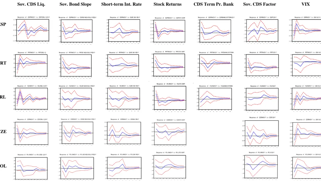
Overall, it appears that there is relevant heterogeneity of the IRFs across the CDS term subcomponents STAT and RW and their volatility regimes. Either the responses of the overall CDS term premium21 are driven by the responses of one subcomponent and/or one volatility regime, or, when the IRFs of the overall CDS term premium are rather muted, we find much sharper IRFs when looking at its STAT and RW subcomponents in regime-dependent fashion. As expected, the responses are more significant for the RW component, in particular in its high-volatility regime. Remarkably, even where there is a response in both high-volatility regimes, the magnitude of the RW response in the high-volatility regime is sometimes as much as ten times higher than in the low-volatility regime, even when the shocks are of similar magnitude.22
All these features become apparent in Figure 3, where we draw the IRFs for each subcomponent in each regime for one sample country – Spain. The IRFs correspond to shocks to two variables: (i) the sovereign bond yield slope and (ii) stock returns. The standard deviations of the two variables are very similar in both volatility regimes (of the CDS term premium subcomponents), so the magnitudes of the IRFs can be compared across regimes. While a shock to the slope of the Spanish bond yield curve only affects the RW component (left column) and not the STAT
20 Alternatively, a macro-finance setting, such as the model of Ang and Piazzesi (2003), could substantially
reduce the estimation errors. However, the restrictive formulation of the observed variables in a typical macro-finance setting could overshadow the economically meaningful interpretation of the interactive market variables. Our goal, in this paper, is to test for an economically meaningful relationship between the unobserved components and a set of observed information that is available to both market participants and policy makers.
21 These results can be found in the working paper version of this paper (Calice et al., 2014).
22 The magnitudes of the IRFs should not be automatically compared in the low- and high-volatility regimes
given that the size of the shocks (the depicted shock corresponds to one standard deviation of each endogenous variable) might differ across these regimes. However, since we define the regimes in terms of the volatility of RW and STAT the variability of the other variables in the VAR might be independent of these regimes. Indeed, the standard deviations of the bond yield slope, short-term interest rate, stock returns, banking CDS term spread, and VIX are very similar in both volatility regimes. Therefore, one can reasonably compare the magnitude of the IRFs in each regime. In contrast, the standard deviations of CDS market liquidity vary substantially across these regimes, as this variable is more directly linked to the volatility regimes of the CDS term premium components.