Modelling COD concentration by using three different ANFIS
techniques
Ozgur Kisi1, Murat Ay2
1Department of Civil Engineering, Canik Basari University, Samsun, Turkey 2
Department of Civil Engineering, Bozok University, Yozgat, Turkey
Abstract
Artificial intelligence (AI) techniques have been successfully performed in many different water resources applications such as rainfall-runoff, precipitation, evaporation, discharge (Q), dissolved oxygen (DO), chemical oxygen demand (COD), biological oxygen demand (BOD), sediment concentration and lake levels by many researchers over the last three decades. In this study, three different adaptive neuro-fuzzy inference system (ANFIS) techniques, ANFIS with fuzzy clustering (ANFIS-FCM), ANFIS with grid partition (ANFIS-GP) and ANFIS with subtractive clustering (ANFIS-SC), were developed to estimate COD concentration by using various combinations of daily input important variables water suspended solids (SS), discharge (Q), temperature (T) and pH. Root mean square error (RMSE), mean absolute error (MAE) and determination coefficient (R2) statistics were used for the comparison criteria. Training, testing
and validation phase’s results of the optimal ANFIS models were also graphically compared
each other. Comparison of the results indicated that the ANFIS-SC(1,0.3,1) model whose input is water SS was found to be slightly better than the other models in estimation of COD according to the comparison criteria in testing phase. In the validation phase, however, ANFIS-FCM(1,3,gauss,1) model performed slightly better than ANFIS-GP(3,trimf,constant,1) and ANFIS-SC(1,0.3,1) models. It can be said that three different ANFIS techniques provide similar accuracy in estimating COD.
Introduction
Analysis of water quality is required to be evaluated according to the national or international standards [1-4] and it should be considered physical, chemical, biological and heavy metals parameters of water [5-9] according to the using purposes as well. These parameters are water pH, DO, electrical conductivity (EC), temperature (T), biological oxygen demand (BOD5), COD, chloride, total phosphate, nitrite, nitrate, ammonia, ions, heavy metals,
total salt concentration, fecal, coliform, and so on. For instance, BOD5is measure of the amount
of biochemical degradable organic matter presented in a water sample. Temperature affects the density of water, the solubility of constituents, pH, specific conductance, the rate of the chemical reactions, and biological activity in water. The other important parameter, the pH value, is controlled by interrelated chemical reactions that produce or consume hydrogen ions [5-6]. The pH of a solution is a measure of the effective hydrogen-ion concentration. COD is a measure of the oxygen equivalent of the organic matter in a water sample that is susceptible to oxidation by a strong chemical oxidant, such as dichromate. EC is the measure of electric conductance ability. This parameter is a direct indicator of the ion content (dissolved salts) in the water. Turbidity is often expressed as total suspended solids (TSS), and TSS can adversely affect stream ecosystems by limiting the light penetration and transparency critical aquatic flora. Water bodies have high transparency values typically have good water quality. DO is important for the healthy
functioning of aquatic ecosystems. Fecal coliform is a bacteriological parameter of water and is used as an indicator of the sanitary quality of the water. Also COD, TSS, Q, BOD5 and pH
parameters are very important to determine system types and volume of a treatment plant [10-14].
AI techniques have been performed water resources especially in non-linear problems and these techniques can be considered as an alternative method in modelling water parameters. For instance, AI techniques have been studied by many researchers in modelling rainfall-runoff, precipitation, evaporation, discharge, DO, BOD5and COD concentration, depth integrated DO,
sediment concentration and lake levels [15-32] over the last three decades. For instance, Lee et al. [33] developed a fuzzy system to determine stream water quality. Dahiya et al. [34] investigated the application of fuzzy set theory for decision-making in the assessment of physic-chemical quality of groundwater for drinking purposes. Application of fuzzy rule based optimization model was illustrated with 42 groundwater samples collected from the 15 villages of Ateli block of southern Haryana, India. Altunkaynak et al. [35] used the historical records of monthly DO, and they modelled DO fluctuations in Golden Horn in Turkey by using Takagi-Sugeno [41] fuzzy logic approach. And, there are also some studies for wastewater treatment plant (WWTP) to model water parameters such as COD, BOD, TSS etc. For instance, Oliveira-Esquerre et al. [36] investigated to model the water BOD in the output stream of a local biological WWTP for the pulp and paper industry in Brazil. Hamed et al. [37] enhanced to estimate the performance ANN models using water BOD, COD and SS collected from a conventional treatment plant in Cairo, Egypt. Mjalli et al. [38] investigated and modelled water BOD, COD and TSS parameters of the Doha West WWTP, State of Qatar by using neural network modelling method. They used these parameters as an input or output variables for the ANNs model structures. Data that they used in models is one-year period. And, measurements were taken for every 5-day. Akratos et al. [39] tried to model BOD and COD removals in five similar pilot-scale horizontal subsurface flow constructed wetlands, and the data used is the two-year period. Kotti et al. [40] developed the fuzzy logic-based method to assess organic matter (BOD and COD concentration) removal efficiency by using 1600 experimental data collected in a 2-year period in five pilot-scale free water surface constructed wetlands.
The main objective of this paper is to analyze and model COD concentration by ANFIS modelling techniques, ANFIS-GP, ANFIS-SC and ANFIS-FCM. Water SS, temperature, pH, Q and COD data from WWTP, at Adapazari province, in Turkey are used in this application. In this context, performances of methods are compared with each other by using statistical criteria. Within the concept of this study, the basic information related study area are presented in the Chapter 2; ANFIS techniques are summarized in the Chapter 3; results of the models are discussed in the Chapter 4; and conclusions are revealed in the Chapter 5.
Materials
Daily measured water SS, T, pH, Q and COD in the upstream of the Adapazari Municipal WWTP located in Marmara region of Turkey are used in this study. Data covers the period between January 2004 and December 2006. The coordinates of the treatment plant are Latitude 40°50'54.24" and Longitude 30°19'40.02". Marmara region has many industrial enterprises and is the most important region of Turkey in terms of population, exporting, importing and marketing systems. Capacity of treatment plant is 198800 m3/day and 271941 m3/day for dry and wet weather, respectively. It is thought that approximately 932 m3/day at full capacity 30%
Black Sea, North of the Turkey. Before this treatment plant was built in 2003, there were many fish dead, agricultural degeneration in this region owing to pollutions.
Methodology
ANFIS techniques, explained in the following chapter, is used to model COD concentration for this treatment plant. It is also used both to determine the accuracy of methods and to model COD as an alternative approach for this process because determination of COD concentration in laboratory is difficult work. For that, it is meaningfully considered that water parameters pH, T, SS and Q are both statistically and physically and chemically, and the correlation coefficients of them are also calculated with COD. And then, the most critical water parameters pH, T, SS and Q were chosen to form models.
Adaptive neuro-fuzzy inference system (ANFIS)
Technically, this method works similar to the neural networks, and it provides a method for the fuzzy modelling procedure to learn information about a data set. And, this method consists of fuzzy logic (FL) approach as well (in MATLAB). FL [43] is the comprehensive version of classical logic. The basic difference between classical logic and FL is that classical logic gives an output as either 0 or 1 but FL can give a continuous output. FL [43-45] system models a system with the help of a fuzzy rule or rules. Fuzzy rules are the expressions that state
the relationship between the system’s inputs and outputs depending on the linguistic variables
and in the form of if-then statements. ANFIS technique [46] is also a network structure consisting of a number of nodes connected through directional links. Each node has a node function with adjustable or fixed parameters. Learning or training phase of network is a process to determine parameter value to sufficiently fit the training data. In addition, ANFIS method divides into 2 methods to generate FIS: grid partition and subtractive clustering method. ANFIS-GP is the major training routine for Sugeno-type fuzzy inference systems. It uses a hybrid learning algorithm to identify parameters of Sugeno-type fuzzy inference systems. It applies a combination of the least-squares method and the back propagation gradient descent method for training FIS membership function parameters to emulate a given training data set. It can also be invoked using an optional argument for model validation. The type of model validation that takes place with this option is a checking for model overfitting, and the argument is a data set called the checking data set. ANFIS-SC method is if you do not have a clear idea how many clusters there should be for a given set of data, SC is a fast, one-pass algorithm for estimating the number of clusters and the cluster centres in a set of data. The cluster estimates, which are obtained from the subclust function, can be used to initialize iterative optimization-based clustering methods and model identification methods (like ANFIS). The subclust function finds the clusters by using the SC method. The genfis2 function builds upon the subclust function to provide a fast, one-pass method to take input-output training data and generate a Sugeno-type FIS that models the data behaviour [41 and 45]. The other method ANFIS-FCM is integration with fuzzy c-means (FCM) algorithm (genfis3 function in MATLAB). ANFIS-FCM is a method which can cluster data based on ANFIS method. The combined method consists of the FCM (fuzzy c-means) clustering algorithm and ANFIS method. In the first step, data are clustered by FCM algorithm and then ANFIS method is applied on the clustered data [43-50].
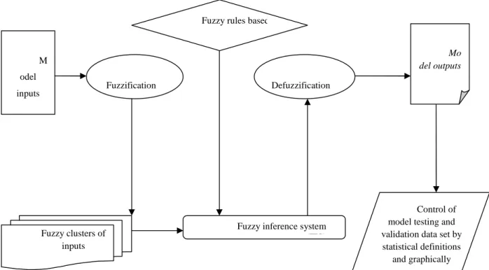
Each ANFIS method has training, testing and validation phases for this problem (Figure 1). In Figure 1, formed as a code file in the MATLAB program and designed user friendly, model inputs phase consists of data of problem, and all these data go to fuzzification phase of system. Then, all parameters data are fuzzificated by using triangular, gauss, trapezoidal, sigmoid etc. membership functions between 0 and 1 degree according to type of problem. Then, optimum rule based is determined either by user or the method used. All systems come to fuzzy inference system (FIS) step. The last defuzzification phase is also step where fuzzy numbers are
converted to the real numbers. And then, model’s results were compared with the measured data
for testing and validation data set by using both statistical definitions and graphically. Generally, it is used three data sets to solve for any a problem. These sets are training set which is used to train for the model, testing and validation sets which are used to calibrate for the model (Figure 1).
Results and discussions
In this study, the MATLAB Neural Network Toolbox was used for the implementation of the ANFIS methods. All of the functions and the require operators were written as a code file in MATLAB. Total 64 different models were evaluated for the ANFIS-SC technique to find the optimal model according to the input combinations, membership functions, epochs, spread coefficient (from 0.1 to 1). In the same way, 64 different models were also evaluated to find out the best ANFIS-GP model for various combinations. The other method ANFIS-FCM is also integration with FCM algorithm (genfis3 function). ANFIS-FCM is a method which can cluster data based on ANFIS method. The silhouette plot method is used in
M odel
inputs Fuzzification Defuzzification
Fuzzy clusters of inputs
Fuzzy rules based
Fuzzy inference system (FIS)
Mo del outputs
Figure 1 Schematic flow of the fuzzy inference system (FIS)
Control of model testing and validation data set by statistical definitions
close to 1. Results of the validation phase of the models are also graphically compared in Figure 2 in the form of time series and scatter plots.
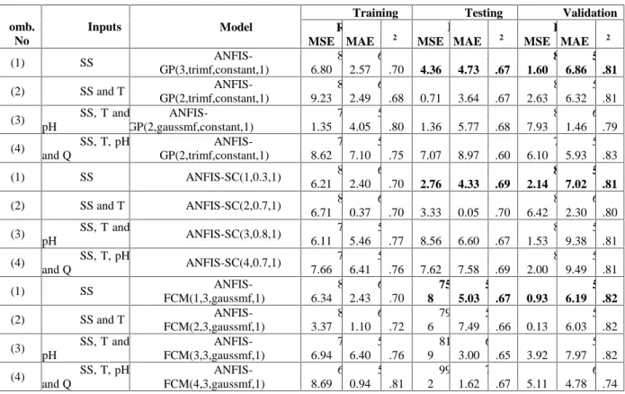
Table 1 RMSE, MAE and R2 statistics of the ANFIS-GP, ANFIS-SC and ANFIS-FCM models in training, testing and validation phase for Adapazari Wastewater Treatment System in modelling COD concentration
C omb.
No
Inputs Model
Training Testing Validation
R MSE MAE R 2 R MSE MAE R 2 R MSE MAE R 2 (1) SS ANFIS-GP(3,trimf,constant,1) 8 6.80 6 2.57 0 .70 7 4.36 5 4.73 0 .67 8 1.60 5 6.86 0 .81 (2) SS and T ANFIS-GP(2,trimf,constant,1) 8 9.23 6 2.49 0 .68 8 0.71 5 3.64 0 .67 8 2.63 5 6.32 0 .81 (3) SS, T and pH ANFIS-GP(2,gaussmf,constant,1) 7 1.35 5 4.05 0 .80 8 1.36 5 5.77 0 .68 8 7.93 6 1.46 0 .79 (4) SS, T, pH and Q ANFIS-GP(2,trimf,constant,1) 7 8.62 5 7.10 0 .75 8 7.07 5 8.97 0 .60 7 6.10 5 5.93 0 .83 (1) SS ANFIS-SC(1,0.3,1) 8 6.21 6 2.40 0 .70 7 2.76 5 4.33 0 .69 8 2.14 5 7.02 0 .81 (2) SS and T ANFIS-SC(2,0.7,1) 8 6.71 6 0.37 0 .70 8 3.33 6 0.05 0 .70 8 6.42 6 2.30 0 .80 (3) SS, T and pH ANFIS-SC(3,0.8,1) 7 6.11 5 5.46 0 .77 7 8.56 5 6.60 0 .67 8 1.53 5 9.38 0 .81 (4) SS, T, pH and Q ANFIS-SC(4,0.7,1) 7 7.66 5 6.41 0 .76 7 7.62 5 7.58 0 .69 8 2.00 5 9.49 0 .81 (1) SS ANFIS-FCM(1,3,gaussmf,1) 8 6.34 6 2.43 0 .70 75.9 8 5 5.03 0 .67 8 0.93 5 6.19 0 .82 (2) SS and T ANFIS-FCM(2,3,gaussmf,1) 8 3.37 6 1.10 0 .72 79.0 6 5 7.49 0 .66 8 0.13 5 6.03 0 .82 (3) SS, T and pH ANFIS-FCM(3,3,gaussmf,1) 7 6.94 5 6.40 0 .76 81.2 9 6 3.00 0 .65 8 3.92 5 7.97 0 .82 (4) SS, T, pH and Q ANFIS-FCM(4,3,gaussmf,1) 6 8.69 5 0.94 0 .81 99.3 2 7 1.62 0 .67 9 5.11 6 4.78 0 .74
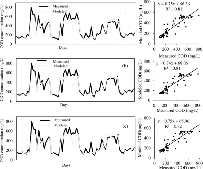
Figure 2 Measured and modelled COD concentrations of the best model in validation phase by (a)ANFIS-GP(3,trimf,constant,1), (b)ANFIS-SC(1,0.3,1) and (c)ANFIS-FCM (1,3,gaussmf,1)
It can be seen from Table 1 and figures that ANFIS-SC (1,0.3,1) model whose input is water SS was found to be slightly better than the other models in estimation of COD according to the comparison criteria in testing phase. This model is defined one input SS, spread coefficient 0.3, and output COD. In the validation phase, however, ANFIS-FCM (1,3,gauss,1) model slightly performed better than the ANFIS-GP(3,trimf,constant,1) and ANFIS-SC(1,0.3,1) models. And, this ANFIS-FCM (1,3,gauss,1) is defined one input SS, 3 (number of clusters), type of membership function (gauss), and output COD. ANFIS-GP(3,trimf,constant,1) model is defined one input SS, type of membership function (triangular) and output function (constant), and output COD. The last model ANFIS-SC(1,0.3,1) is defined one input SS, spread coefficient 0.3, and output COD. It can be said that three different ANFIS techniques provide similar accuracy in estimating COD concentration for this treatment plant.
0 200 400 600 800 Series1 Series2 Days CO D c o n ce n tra ti o n ( m g /L ) Measured Modeled y = 0.75x + 66.36 R² = 0.81 0 200 400 600 800 0 200 400 600 800 M o d ele d C OD (m g /L ) Measured COD (mg/L) y = 0.74x + 68.06 R² = 0.81 0 200 400 600 800 0 200 400 600 800 M o d ele d C OD (m g /L ) Measured COD (mg/L) 0 200 400 600 800 Series1 Series2 Days CO D c o n ce n tra ti o n ( m g /L ) Measured Modeled (b) y = 0.75x + 65.96 R² = 0.82 0 200 400 600 800 0 200 400 600 800 M o d ele d C OD (m g /L ) Measured COD (mg/L) 0 200 400 600 800 Series1 Series2 Days CO D c o n ce n tra ti o n ( m g /L ) Measured Modeled (c) ( a)
Conclusions
Chemical oxygen demand (COD) concentration is both an important water quality parameter and commonly used in aquatic life related to case evaluation. In this study, potential of ANFIS method approach in estimating COD was investigated by using different combinations, methods, functions, epoch and other assumptions to find out optimum model. And, these ANFIS methods, ANFIS-GP, ANFIS-SC and ANFIS-FCM, were compared with each other as well. For that, daily data water suspended solids, temperature, pH, discharge and COD concentration data measured in upstream of the Adapazari Municipal WWTP, Marmara region of Turkey were used in this study. Comparison of the results indicated that the ANFIS-SC(1,0.3,1) model whose input is water SS was found to be slightly better than the other models in estimation of COD in testing phase according to the comparison criteria. In the validation phase, however, the FCM(1,3,gauss,1) model slightly performed better than the ANFIS-GP(3,trimf,constant,1) and ANFIS-SC(1,0.3,1) models. It can be said that three different ANFIS techniques provide similar accuracy in estimating COD for this treatment plant. And, the results showed that the water SS parameter was quite effective on COD concentration. In addition, it can be said that models are quite effective view to model COD as a priori and an alternative point of view. And, these models can be used a priori tool to evaluate COD only available water SS parameter without doing laboratory studies for this treatment plant as well.
Acknowledgement: We sincerely thank to the staff of the municipal WWTP in
Adapazari, in Turkey, for the data observation, processing, management, and for MSc thesis
written by Sebile Açıkalın [51].
References
[47] EPA United State Environmental Protection Agency (1994). Water Quality Standards
Handbook, 2nd ed.
[48] Council Directive 98/83/EC of 03 November 1998 on the quality of water intended for human consumption. OJ L 330.
[49] Official paper (2004). Water Pollution Control Regulations (WPCR, in Turkish). [50] WHO, (2008). Guidelines for drinking-water quality, World Health Organization.
[51] Hem, J.D. (1985). Study and Interpretation of the Chemical Characteristics of Natural Water, U.S. Geological Survey, Water Supply Paper 2254.
[52] Chapman, D. (1992). Water Quality Assessment, 1st ed. London. Chapman and Hall. [53] Wagner, R.J., Boulger, R.W., Oblinger, J.C. Smith, A.B. (2006). Guidelines and Standard
Procedures for Continuous Water-Quality Monitors: Station Operation, Record Computation, and Data Reporting. Techniques and Methods(TM),1-D3. USGS.
[54] Radtke, D.B., Busenberg, E., Wilde, F.D., and Kurklin, J.K. eds. (2003). pH (version 1.2):
U.S. Geological Survey Techniques of Water-Resources Investigations, 9, A6, 6.4, 28p.
[55] Radtke, D.B., Kurklin, J.K., and Wilde, F.D., eds. (2004). Temperature (version 1.2): U.S.
Geological Survey Techniques of Water-Resources Investigations, book 9, chapter. A6,
[56] UNESCO/WHO/UNEP, (1996). Water quality assessment-A guide to use of Biota, Sediments and Water in Environmental Monitoring-2nd Edition, 651p. Edited by
Chapman, D.
[57] Cox, B.A. (2003). A review of dissolved oxygen modeling techniques for lowland rivers.
Science Total Environmental, 314-334.
[58] Metcalf&Eddy, (2004). Wastewater Engineering Treatment and Reuse, Fourth Edition. [59] Mullholand, P.J., Houser, J.N. and Maloney, O.K. (2005). Stream diurnal dissolved
oxygen profiles as indicators of in-stream metabolism and disturbance effects: fort Benning as a case study. Ecological Indicator 5, 243-252.
[60] Neal, C., House, W.A., Jarvie, H.P., Neal, M., Hilla, L. Wickham, H. (2006). The water quality of the River Dun and the Kennet and Avon Canal. J of Hydrol, 330, 166-170. [61] ASCE Task Committee on Application of Artificial Neural Networks in Hydrology,
(2000a). Artificial neural networks in hydrology I: Preliminary concepts. Journal of
Hydrologic Engineering 5 (2), 115-123.
[62] ASCE Task Committee on Application of Artificial Neural Networks in Hydrology, (2000b). Artificial neural networks in hydrology II: Hydrologic applications. Journal of
Hydrologic Engineering 5(2), 124-137.
[63] Maier, H.R. and Dandy, G.C. (1996). The use of artificial neural networks for prediction of water quality parameters. Water Resource Research 32(4), 1013-1022.
[64] Hagan M.T. and Menhaj M.B. (1994). Training feed forward networks with the Marquardt algorithm. IEEE Transactions on Neural Networks 5(6), 861-867.
[65] Cherkassy, V., Krasnopolsky, V., Solomatine, D.P. and Valdes, J. (2006). Computational intelligence in earth sciences and environmental applications: Issue and challenges. Neural
Networks 19, 113-121.
[66] Cancelliere, A., Giuliano, G., Ancarani, A., Rossi, G. (2002). A neural network approach for deriving irrigation reservoir operating rules. Water Res Manag 16(1), 71-88.
[67] Chang, F. J. and Chen, Y. T. (2009). Adaptive neuro-fuzzy inference system for prediction of water level in reservoir, Advance in Water Resources, 29, 01-10
[68] Dawson, C.W., Abrahart, R.J., Shamseldin, A.Y. and Wilby, R.L. (2006). Flood estimation at ungauged sites using artificial neural networks. J of Hydrol 319, 391-409. [69] Kumar, DN., Raju, KS., Sathish, T. (2004). River flow forecasting using recurrent neural
Networks. Water Resource Management 18(2), 143-161.
[70] Rajaee, T., Mirbagheri, S.A., Zounemat-Kermani, M., Nourani, V. (2009). Daily suspended sediment concentration simulation using ANN and neuro-fuzzy models.
Science of the Total Environment 407, 4916-4927.
[71] Banerjee, P., Singh, V.S., Chatttopadhyay, K., Chandra, P.C. and Singh, B. (2011). Artificial neural network model as a potential alternative for groundwater salinity forecasting. Journal of Hydrology 398, 212-220.
[74] Kisi, O. (2009). Modeling monthly evaporation using two different neural computing techniques. Irrigation Science, 27, 417-430.
[75] Duque-Ocampo, W., Ferré-Huguet, N., Domingo, J. L. and Schuhmacher, M. (2006). Assessing water quality in rivers with fuzzy inference systems: A case study. Environment
International 32, 733-742.
[76] Rehana, S. and Mujumdar, P.P. (2009). An imprecise fuzzy risk approach for water quality management of a river system. J of Environ Manag, 90, 3653-3664.
[77] Icaga, Y. (2007). Fuzzy evaluation of water quality classification. Ecological Indicators 7, 710-718.
[78] Yan, H., Zou, Z. and Wang, H. (2010). Adaptive neuro fuzzy inference system for classification of water quality status, J Environ Sci 22(12), 1891-1896.
[79] Lee, D.S., Park, J.M., (1999). Neural network modeling for on-line estimation of nutrient dynamics in a sequentially-operated batch reactor. Journal of Biotechnology 75, 229-239. [80] Dahiya, S., Singh, B., Gaur, S., Garg, V.K. and Kushwaha, H.S. (2007). Analysis of
groundwater quality using fuzzy synthetic evaluation. J of Hazar Mat 147, 938-946.
[81] Altunkaynak, A., Özger, M. and Çakmakçı, M. (2005). Fuzzy logic modeling of the
dissolved oxygen fluctuations in Golden Horn. Ecological Modeling 189, 436-446.
[82] Oliveira-Esquerre, K.P., Mori, M., Bruns, R.E. (2002). Simulation of an industrial wastewater treatment plant using artificial neural networks and principal components analysis. Brazilian Journal of Chemical Engineering 19, 365-370.
[83] Hamed, M., Khalafallah, M.G., Hassanein, E.A. (2004). Prediction of wastewater treatment plant performance using artificial neural net-work. Environmental Modelling
and Software 19, 919-928.
[84] Mjalli, F.S., Al-Asheh S. and Alfadala, H.E. (2007). Use of artificial neural network black-box modeling for the prediction of wastewater treatment plants performance. Journal of
Environmental Management 83, 329-338.
[85] Akratos, C.S., Papaspyros, J.N.E. and Tsihrintzis, VA. (2008). An artificial neural network model and design equations for BOD and COD removal prediction in horizontal subsurface flow constructed wetlands. Chemical Engineering Journal 143, 96-110.
[86] Kotti, I.P., Sylaios, G.K., Tsihrintzis, V.A. (2013). Fuzzy logic models for BOD removal prediction in free-water surface constructed wetlands. Ecol Eng. 51, 66-74. [87] Takagi, T. and Sugeno, M. (1985). Fuzzy identification of systems and its applications to
modeling and control. IEEE Trans Syst Man Cybernet 15, 116-32.
[88] Eren, B., Suroğlu, B., Ateş, A., İleri, R. and Keleş, R. (2007). Evaluation of
characterization of Adapazari municipial wastewater treatment system. II. Environmental
issues for university students, Fatih University, Istanbul, TURKEY.
[89] Fuzzy Logic Toolbox 2 User’s Guide, (2007), MATLAB, 299p. Version 2.2.6.
[90] Ross, T. J. (2004). Fuzzy logic with engineering applications. McGraw-Hill, Inc. [91] Zadeh, L.A. (1965). Fuzzy Sets. Information Control 8 (3), 338-353.
[92] Jang, J.S.R. (1993). ANFIS: Adaptive-Network-based Fuzzy Inference Systems. IEEE
Transactions on Systems, Man, and Cybernetics, 23(3), 665-685.
Compact Well-Separated Clusters, Journal of Cybernetics, 3, 32-57
[94] Bezdek, J. C. (1981). Pattern Recognition with Fuzzy Objective Function Algorithms,
Plenum Press, New York.
[95] Miyamoto, S., Ichihashi, H. and Honda, K. (2008). Algorithms for Fuzzy Clustering: Methods in c-Means Clustering with Applications, Springer, 248p.
[96] Oliveira, J.V. and John, W.P. (2007). A comprehensive, coherent, and in depth presentation of the state of the art in fuzzy clustering. Wiley & Sons, 454p.
[97] Açıkalın, S. (2007). Estimation of efficiency urban wastewater treatment plant by artificial
neural network. Msc Thesis, 140p., Department of Environmental Engineering, Graduate School of Natural and Applied Sciences, Sakarya University, Turkey.