Predatory Lending
Rodrigue Mendez
To cite this version:
Rodrigue Mendez. Predatory Lending. 2012. <hal-00991948>
HAL Id: hal-00991948
http://hal.univ-lille3.fr/hal-00991948
Submitted on 16 May 2014
HAL is a multi-disciplinary open access archive for the deposit and dissemination of sci-entific research documents, whether they are pub-lished or not. The documents may come from teaching and research institutions in France or abroad, or from public or private research centers.
L’archive ouverte pluridisciplinaire HAL, est destin´ee au d´epˆot et `a la diffusion de documents scientifiques de niveau recherche, publi´es ou non, ´emanant des ´etablissements d’enseignement et de recherche fran¸cais ou ´etrangers, des laboratoires publics ou priv´es.
Hgh
Document de travail
Lille 1 І Lille 2 І Lille 3 І
[2012–17]
“Predatory Lending”
“Predatory Lending”
Rodrigue Mendez
Rodrigue Mendez
PRES Université Lille Nord de France, Université du Littoral, Laboratoire EQUIPPE
EA 4018, Villeneuve d’Ascq, France.
Predatory Lending
Rodrigue Mendez ∗May 2012
Abstract
This paper studies the equilibrium predatory practices that may arise when the borrowers have behavioral weaknesses. Rational lenders offer short term contracts that can be renewed at the cost of paying a penalty fee. We show how the optimal contracts depend on the degree of na¨ıvet´e of the time inconsistent customers. Penalty fees have a dual role : they increase market share by providing a useful commitment device to time-inconsistent but otherwise rational borrowers ; they are also a source of revenue from the semi-na¨ıve borrowers who understand the need for commitment but fail to forecast their future time discount factor. We also show that perfect com-petition does not eliminate predatory practices, since the equilibrium contract entails a subsidized (below marginal cost) short-term loan that can only be profitable if a fraction of the borrowers end up paying the penalty fee.
JEL : D03, D18, D49, D86
Keywords : hyperbolic discounting, time inconsistency, sophistication, partial na¨ıvet´e, exploitative contracts, credit cards
1
Introduction
The paper focuses on the equilibrium predatory practices that may arise when the bor-rowers have behavioral weaknesses. Our main assumption is that the borbor-rowers have the (δ, β,β˜) quasi-hyperbolic preferences introduced by O’Donoghue and Rabin (1999a, 2001). This assumption has two components. First, the quasi-hyperbolic preferences imply that the borrowers have a self-control problem (their inability to resist the urges of immedi-ate consumption), which may lead to time-inconsistent choices, since their preferences are time-varying. Second, the borrowers are not fully aware of the dynamics of their prefer-ences (they tend to overestimate their future discount factor). This second hypothesis, which we label the na¨ıvet´e hypothesis will turn out to be a crucial element of the analysis. The lending institutions are fully rational. They are aware of the behavioral weaknesses of their customers and will devise contracts that take advantage of those weaknesses. The
purpose of the paper is to make a systematic exploration of those contracts, which we label exploitative contracts. We assume that the lending institutions offer short-terms lending contracts that can be renewed, at a cost. The contracts have therefore two main
characteristics : the interest rateR and the roll-over feeF.
We show that the optimal exploitative contracts depend crucially on the degree of na¨ıvet´e of the borrowers. Sophisticated individuals (those who are fully aware of the dynamics of their preferences) cannot be fooled. They are offered contract with positive fees, where the fees are used as a commitment device (that allows them to implement their optimal consumption path). This is no longer the case with na¨ıve borrowers. Fully na¨ıves don’t understand the commitment value of the fees, and therefore focus only on the interest rate (since they don’t expect to pay the fee). The optimal contract is one with high interest rates and zero fees. Partially na¨ıves understand the commitment value of the fee, but can nevertheless be fooled, since they overestimate their future discount factor. The optimal contract is one with high interest rates and a positive fee, that the borrowers end-up paying in some configurations. Deceitful contracts thus only arise with partially na¨ıves borrowers in the monopoly case.
Most authors argue that competition should eliminate the predatory practices. We show that this is not the case in our framework. Perfect competition allows the sophisti-cated consumers to take the whole surplus (the equilibrium interest rate falls to marginal cost and the firm’s profits are zero at equilibrium). But predatory contracts do persists as long as a there is a small fraction of na¨ıves. The optimal equilibrium contract is clearly based on deceit, since the firms offer short term loans at discount rates (rates below marginal cost) that can only be profitable if a fraction of customers roll over the loan and thus end up paying the penalty fee they did not expect to pay. Perfect competition implies that the lending firms do not profit from their predatory practices in equilibrium (profits are null in equilibrium). The main beneficiaries of the deceitful contracts are the sophisticated borrowers who benefit from the discount rates, and use the penalty fee as a commitment device.
This paper is related to the growing literature on contracting with boundedly rational agents which started with the seminal contribution of Della Vigna and Malmendier (2004) (henceforth referred as D&M). Their model is a three period version of the (δ,β, ˜β) model of O’Donoghue and Rabin (1999a, 2001). They show that the optimal two-part contract depends on the nature of the good provided by the firm. They distinguish two types of
goods : leisure good, which provides current benefits, but have future costs andinvestment
good, that have current costs and future benefits. A monopoly that sells a leisure good
should choose a low entry cost and a high usage cost (i.e. above marginal cost) to take advantage of the na¨ıve’s tendency to underestimate their future usage. If the firm sells an
investment good, the optimal pricing policy is the converse : a high fixed cost and a low usage cost (below marginal cost), in order to exploit the semi-na¨ıves tendency tendency to overestimate their future usage as well as their demand for commitment (which is provided by the high entry cost).
Heidhues and K˝oszegi (2009) focus on over-commitment. Semi-na¨ıves individuals who
want to avoid the future consumption of an harmful good (a leisure good using D&M terminology), have the opportunity to buy a costly commitment technology. But most of them end up buying the good anyway as they underestimate their lack of self-control. The authors show that higher sophistication (greater awareness of the self control problem) is often worse than full na¨ıvet´e, since it increases the spending on commitment without
preventing the consumption of the harmful good. Heidhues and K˝oszegi (2010) studies
full competition, their results are similar to D&M : the equilibrium contracts have low teaser rates for short term loans and large penalty fees for those who fall behind on their payment schedule.
The subject of Gottlieb (2008) is competition over time-inconsistent consumers. They point that the impact of competition on the pricing of leisure goods depends crucially on the customer’s switching costs. D&M pricing (lump-sum transfers to bait customers and above marginal cost usage price) requires exclusive contracts. When those contracts are not feasible, firms choose marginal cost pricing (and zero lump-sum transfers).
Others significant contributions are Eliaz and Spiegler (2006) and Gabaix and Laibson (2006). Both show how firms may profit by devising contracts that discriminate between sophisticated and na¨ıve customers. In the Eliaz & Spiegler setting, the agents differ in their ability to forecast the change in their future tastes. The optimal menu of contract provides perfect commitment devices for the sophisticated consumers, and exploitative contracts for the na¨ıve. Gabaix & Laibson analyze the issue of informational shrouding. Firms offer a base good and and add-ons. They show how firms may exploit myopic consumers through marketing schemes that offers cheap base goods and shroud high-priced add-ons, and how sophisticated consumers profit from those schemes. They also show that competition does not eliminate shrouding.
Empirical evidence on the pricing of investment good is provided by Della Vigna and Malmendier (2006) in the context of the health club markets. Della Vigna and Malmendier (2004) also gives (second hand) evidence of the pricing of leisure goods with switching costs (credit cards, mobile phones). Gottlieb (2008) provides evidence of the pricing on leisure goods with switching costs in competitive industries (Tobacco and and alcohol industries). Gabaix and Laibson (2006) provide evidence on shrouding in the retail banking industry and in the printer market. First hand evidence on the practices of the credit card industry can be found in Ausubel (1991) and Shui and Asubel (1995) A full presentation of the payday loan market can be found in Stegman (2007) and Agarwal et al. (2009).
The paper proceeds as follows. Section 2 presents the model. Sections 3 and 4 analyze the optimal pricing strategy under monopolistic conditions. The form and the impact of the contract depend crucially on the degree of na¨ıvet´e of the borrowers. Section 3 estab-lishes the optimal contract for sophisticated borrowers, whereas section 4 show how firms can take advantage of the borrower’s na¨ıvet´e. Section 5 analyzes the effect of competition on the equilibrium pricing strategies. Section 6.1 studies the impact of predatory lending on the welfare of the borrowers under monopoly and competition. Section 7 concludes. All proofs omitted in the main text are given in the appendix.
2
The Model
2.1 Intertemporal Preferences
We assume that the borrowers have (δ,β, ˜β) quasi-hyperbolic intertemporal preferences At timet, the present value of the flow of future utilities (us)s≥t is :
ut+β ∑
s≥t+1
δs−tu
s (1)
whereδ ≤1 is the long-run discount factor andβ ≤1 is the short-run one. β <1 results
from a self-control problem (the inability to resist to the urges of immediate consumption) Quasi-hyperbolic preferences (henceforth referred as q-hyper pref) imply that discounting
at time t+ 1. Time consistency thus requiresβ = 1. β can therefore be considered as a measure of the degree of time inconsistency of the agent.
The parameter β ≤ β˜ ≤ 1 is the expected short-run discount factor. A na¨ıve agent
overestimate his future discount factor (he expects - erroneously - to have the discount function 1,βδ,˜ βδ˜ 2, ..in all future periods). An agent with ˜β = 1 is said to be fully na¨ıve,
whereas an agent with ˜β = β is a sophisticated one. ˜β −β is therefore a measure of
the degree of the agent’s na¨ıvet´e (the tendency to believe that his lack of self-control is temporary)
For the sake of simplicity we assume from now on that : (i) individuals live three periods ; (ii) their instantaneous utility is linear ; and (iii) the long-run discount factor is
δ= 1.
2.2 The lending institution
The lending institution is a fully rational profit maximizing monopoly. The firm has zero fixed and marginal costs (the lending institution can borrow at zero cost from the central bank, her discount rate is thus zero). The firm proposes two types of borrowing contracts : a short-run contract and a long run one.
• The short-run contract (henceforth referred as SR contract). The firm lends for
one period (at interest rate R), and gives the individual the possibility to rollover
the debt for one period more. The option to rollover is costly. An individual that
chooses to rollover must pay a penalty F on the outstanding debt. The total cost
of borrowing is therefore R for the borrowers that repay in time and R(R+F) for
the borrowers that choose to rollover. Profit is therefore R−1 per unit lent in the
former case, andR(R+F)−1 in the latter case (recall that the firm’s discount rate
is zero).
• The long-run contract (LR). The firm lends for two periods at interest rate R (per
period), which yield a profit equal to R2−1.
The firm is fully aware of the self-control and na¨ıvet´e problems. Contracts are designed to exploit them.
2.3 The distribution of (β, β˜)
The borrowers are heterogenous. There is a continuum of agents of size one. We
assume that the short-run discount factorβ are uniformly distributed on the support [β0,
1], whereβ0 is the short-run discount factor of the most impatient borrower.
We also assume that the expected short-run discount factor ˜β is an increasing function
ofβ, with : ˜ β(β) = { ¯ β if β <β¯ β if β≥β¯ (2)
This formulation implies that all individuals withβ <β¯are na¨ıves, whereas all individual
withβ≥β¯are fully sophisticated. The na¨ıvet´e and the lack of self-control are correlated
since ˜β−β is decreasing in β.
3
Contracting with sophisticated borrowers
We assume in this section that all the borrowers are fully sophisticated ( ¯β = β0).
penalties increase both the profit of the firm and the welfare of the borrowers.
3.1 The optimal contract when penalties are not allowed
At time t= 1, the net benefit of borrowing one unit is (1−βR) if the agent repays
at time t= 2, and (1−βR2) if the agent repays at time t= 3. One-period borrowing is
thus better for the agent (the converse is true for the firm, who earnsR−1 with the short
term contract andR2−1 with the long term one).
All agents with β ≤ 1/R wish to borrow for one period. Yet, sophisticated agents
know that their intertemporal preferences will change at time t = 2. The net benefit of
deferring the repayment, which isR−R= 0 at timet= 1, will be, at timet= 2, (1−βR).
Therefore all agents who choose to borrow for one period at time t = 1 will rollover at
timet= 2, and end up payingR2 at time t= 3. Since two-period borrowing is profitable
only for agents withβ ≤1/R2, all agents withβ >1/R2 will choose not to borrow. Figure 1 represents the choice of the individuals in the [β0,1] space.
1/R
1/R
1
β
02-period
β
2Contract
Figure 1: The Choices of sophisticated borrowers (F = 0)
This implies that the interest rate chosen by the firm must not exceed 1/√β0 (since
no one borrows whenβ0R2 >1), in which case the firm earnsR2−1 per unit lent to each
agent in the interval [β0,1/R2]. Assuming that the agents can borrow at most one unit1,
the firm’s profit function Π(R, F) writes :
Π(R,0) =
{
(R2−1)G(1/R2) if 1≤R≤1/√β0
0 if R >1/√β0 (3)
whereG(β) = (β−β0)/(1−β0) is the cumulative distribution function ofβ. It is easy to
show that the profit function is concave in the interval [1,1/√β0]. The maximum profit is
reached whenR=R∗
0≡(1/β0)1/4.
3.2 The optimal contract with penalties
Introducing penalties will increase both the firm’s profit and the average welfare of the borrowers.
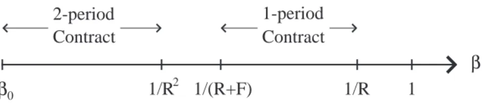
The reason is that penalties are used as a commitment device by the borrowers. Recall that all borrowers withβ∈]1/R2,1/R[ wish to borrow (since 1−βR >0) but choose not to since they know that they will rollover, and rollover is not profitable for them. A penalty
changes the net benefit of deferring repayment att= 2, which is now 1−β(R+F), which
implies that rollover is no longer profitable for all agents withβ > 1/(R+F). Knowing
this, all agents withβ∈[1/(R+F),1/R] choose to borrow for one period. The behavior
of the other agents is not modified. Figure 2 represents the choice of the sophisticated borrowers in the [β0,1] space when F is positive.
1
1/R
1/R
1
β
02-period
1-period
1/(R+F)
β
2Contract
Contract
Figure 2: The Choices of sophisticated borrowers (F >0)
Let’s compute the profit, assuming that the interest rate isR=R∗
0and that 1/(R0∗)2 ≤
1/(R∗
0+F). The profit of the firm is the sum of the profit made on the 2-period contracts
Π(R∗
0,0) and the profit made on the one-period contract.
Π(R∗
0, F) = Π(R∗0,0) + (R−1) [G(1/R∗0)−G(1/(R0∗+F))] (4)
which is clearly an increasing function of F. The maximum is reached when 1/(R∗
0)2 =
1/(R∗
0+F)⇒F0∗ =R∗0(R∗0−1). This results from the fact that choosing a penalty above
F∗
0 allows the individuals in the interval [1/(R∗0+F),1/(R∗0)2] to replace their 2-period
contract by one-period ones, which clearly reduces the profit of the firm by (R∗
0)2−R∗0 per
contract.
To compute the optimal (RS, FS) we must write the profit function. Assuming that
F <1/β0−1/√β0, the profit function writes :
Π(R, F) = (R2−1)G( 1 R+F ) + (R−1)[G(1 R ) −G(R+1F)] if 1≤R<RF (R2−1)G( 1 R2 ) + (R−1)[G(1 R ) −G(R+1F)] if RF≤R<√1 β0 (R−1)[G(1 R ) −G(R+1F)] if 1 √β 0≤R< 1 β0−F (R−1)G(1 R ) if 1 β0−F≤R≤ 1 β0 (5)
where RF = (1 +√1 + 4F)/2 is the unique positive solution of the equation 1/R2 =
1/(R+F). 2
Proof. It is obvious that no one borrows for R > 1/β0. One period contracts are
chosen by all individuals when 1/β0−F ≤R≤1/β0. This results from the fact that they
are profitable for all individuals (since βR < 1, ∀β) and that the borrowers know that
they will not rollover (since β(R+F) >1, ∀β). The profit is (R−1) times the number
of contracts G(1/R). Note that 2-period contracts are nor an alternative since βR2 >1,
∀β. One-period contact are still the only alternative when 1/√β0 ≤R ≤ 1/β0−F, but
they will be chosen only by a fraction of the individuals, since all the agents will β such
that β(R+F) ≤ 1 know that they will rollover. The profit is therefor R−1 times the
number of contractsG(1/R)−G(1/(R+F)). Choosing R≤1/√β0 allows the individual
to choose between one-period and 2-period contracts. One-period contracts will be chosen by all those who don’t expect to rollover (those withβsuch thatβ(R+F)>1), the others will chose either a 2-period contract (ifβR2 <1) or to abstain from borrowing (if 1/R2 <
β <1/(R+F)). The no-borrowing zone disappears when 1/R2 >1(R+F) ⇐⇒R > RF.
Thus the profit isR2−1 times the number of 2-period contracts (G(1/R2) whenR ≥RF,
and G(1/(R+F)) when R < RF) plus R−1 times the number of one-period contracts
G(1/R)−G(1/(R+F)).
2
The restrictionF <1/β0−1/√β0ensures thatRF lies in the interval [1,1/√β0]. We show in appendix
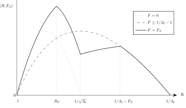
As we can see in figure 3, the maximum profit is reached for RS =RF. The penalty is set at a level that : (i) ensures all agents choose either a one-period contract or a two-period contract ; (ii) avoids the cannibalization of 2-period contracts by one-period contracts. 0 F = 0 F ≥1/β0−1 F =FS RF R Π(R, FS) 1/β0−FS 1/β0 1 1/√β0
Figure 3: The profit function with sophisticated borrowers forF =FS
In the appendix A.2, we show that the optimal (RS, FS) couple is :3
RS = ( 1 β0 )1/3 (6) FS = RS(RS−1) = ( 1 β0 )1/3( 1− ( 1 β0 )1/3) (7)
4
Contracting with na¨ıve borrowers
We first we study the full na¨ıvet´e case ( ¯β = 1). Then we look at the partial na¨ıvet´e
caseβ0 <β <¯ 1
4.1 Full na¨ıvet´e
In this case the potential borrowers don’t expect to rollover (since ˜β(R+F) =R+F >
1, ∀R > 1, F ≥ 0). Thus all the agents who wish to borrow one period (those with
β ≤ 1/R) will do so. Of course, all agents with β < 1/(R+F) will rollover and pay
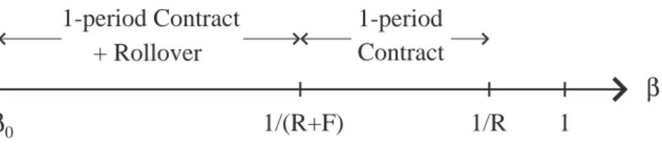
the penalty. Now the firm must balance the additional income generated by the penalty fees and the loss of some 2-period borrowers due to the penalty (recall that the agents in the [1/(R+F),1/R] interval do not rollover). Figure 4 represents the choices of the individuals whenβ0<1/(R+F) :
3
1/R
1
β
01-period Contract
1-period
1/(R+F)
β
+ Rollover
Contract
Figure 4: The Choices of fully na¨ıve borrowers The profit function of the firm writes :
Π(R, F) = { (R(R+F)−1)G( 1 R+F)+(R−1)[G( 1 R)−G( 1 R+F)] if 1≤R< 1 β0−F (R−1)G(1 R) if R≥ 1 β0−F (8)
Proof. All agent withβ ≤1/R borrow for one period. IfR≥1/β0−F the penalty is big
enough to deter rollover for all agents (β(R+F) >1,∀β). The profit is (R-1) times the
number of contracts G(1/R). This is no longer the case for R < 1/β0 −F. The agents
whoseβ <1/(R+F) will rollover and pay the penalty. The profit is (R(R+F)-1) times the
number individual who rolloverG(1/(R+F)) plusR−1 times the number of individuals
who don’tG(1/R)−G(1/(R+F)).
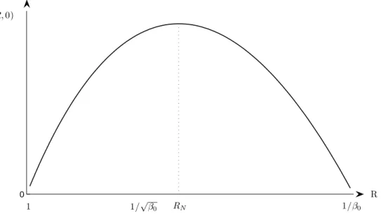
It is easy to show that (i) the firm chooses a contract with zero penalty ( ˜F = 0); and
(ii) the optimal interest rateRN is such that 1/√β0 < RN <1/β0 (see the appendix for
the proof). The figure 5 shows the optimal solution.
The logic of the no-penalty result is straightforward. Introducing a penaltyF leads to
a gain ofF on theG(1/(R+F)) individuals that continue to rollover and a loss ofR2−R
on theG(1/R)−G(1/(R+F)) individuals that no longer rollover. The net gain is :
F×G ( 1 R+F ) −R(R−1) [ G ( 1 R ) −G ( 1 R+F )] = F 1 R+F −β0 1−β0 − R(R−1) 1 R− R+1F 1−β0 = − 1 1−β0 F2 R+F <0
which is always negative. Adding a penalty is therefore never profitable when the borrowers are fully na¨ıve.
0 1 1/β0 R 1/√ β0 Π(R,0) RN
Figure 5: The profit function with fully na¨ıve borrowers
4.2 Partial na¨ıvet´e
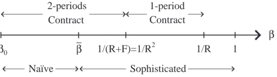
There are three equilibrium configurations in the partial na¨ıvet´e case, which we label : (i) nearly sophisticated ; (ii) sophisticated na¨ıve ; and (iii) nearly na¨ıve. In the following we characterize each configuration (full proofs are given in appendix C).
4.2.1 Configuration 1 : Nearly sophisticated
This is the equilibrium configuration when ¯β is low ( ¯β ∈[β0,β¯1[)4. As can be seen in
figure 6, this configuration is such that ¯β <1/R2= 1/(R+F). Thus all the agents with
β ≤1/(R+F) (rightly) expects to rollover. Recall that the expected discount factor is
˜
β(β) =β ≥β¯for the sophisticated agents and ˜β(β) = ¯β for the na¨ıve ones, which implies that the expected discount factor is small enough ( ˜β(β)<1/(R+F),∀β <1/(R+F)) to send the right signal to the na¨ıve borrowers (do not sign the one-period contract since you will rollover!). Therefore all agents whoseβ >1/(R+F) choose the one-period contract,
whereas those withβ ≤1/(R+F) choose the 2-period contract5 No penalty is ever paid.
The configuration 1 equilibrium is an “honest” equilibrium where no one is fooled, and
the penalty fee F is used as a commitment device for both the na¨ıve and sophisticated
borrowers. The equilibrium (R, F) pair is the same as the one chosen when all individuals
are sophisticated (R =RS = (1/β0)1/3, F =FS =RS(RS−1)).
4The value of ¯β
1 is given in appendix C 5
The firm choosesRsuch that 1/R2
= 1/(R+F) since 1/R2
<1/(R+F) leads to the loss of valuable consumers and 1/R2
>1/(R+F) leads to the cannibalization of 2-period contracts by the less profitable one-period contracts.
1/R
1
β
02-periods
1-period
1/(R+F)=1/R
2β
Contract
Contract
β
_
Naïve
Sophisticated
Figure 6: Configuration 1 : Nearly sophisticated
4.2.2 Configuration 2 : Sophisticated na¨ıves
This is the equilibrium configuration for intermediate ¯β ( ¯β ∈ [ ¯β1,β¯2[) 6. As can be
seen in figure 7, this configuration is such that ¯β = 1/(R +F) > 1/R2. Therefore all
borrowers choose the one-period contracts (no one expects to rollover since ˜β ≥ β,¯ ∀β).
This is the right decision for the sophisticated agents, since they will not rollover (β ≥
1/(R+F),∀β ≥ β¯), and the wrong decision for the na¨ıve ones (since they will rollover and pay the penalty).
1/R
1
β
01-period Contract
1-period
1/(R+F)=
β
+ Rollover
Contract
Naïve
Sophisticated
1/R
2β
_
Figure 7: Configuration 2 : Sophisticated na¨ıve
The penalty has therefore a dual role in configuration 2. The penalty is used as a commitment device for the sophisticated agents (who would choose to abstain from
borrowing ifF = 0), and as a bait for the na¨ıve ones. Note that the optimal behavior for
the na¨ıve agents would be either to borrow for two periods (for those with β <1/R2) or
to abstain from borrowing (for those withβ ≥1/R2).
We show in appendix C that the optimal interest rate and penalty fee are : 7
RSN = √ ¯ β β0−β¯(1−β¯) (9) FSN = 1 ¯ β −RSN = 1 ¯ β − √ ¯ β β0−β¯(1−β¯ (10)
The figure 8 represents the profit as a function ofR when F =FSN.
6
The value of ¯β2 is given in appendix C 7The subscript
0 R
1/√β0 1/β0
Π(R, FS N)
1/β0−FS N
1/β¯−FS N
Figure 8: The profit function with sophisticated na¨ıves.
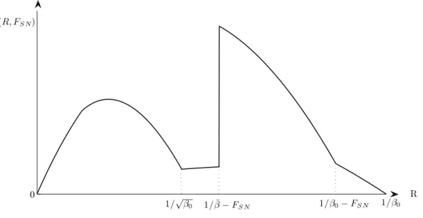
4.2.3 Configuration 3 : Nearly na¨ıve
This is the equilibrium configuration when ¯β is high ( ¯β ∈[ ¯β2,1]). As can be seen in
figure 9, this configuration is such that ¯β ≥1/R. The optimal interest rate is such that :
(i) sophisticated agents do not borrow ; and (ii) all na¨ıve agents borrow for one period and then rollover in the second period. As in fully naive case, the choice of the optimal penalty fee must balance the additional income generated by the fee and the loss of some two-period contracts caused by this fee. We show in appendix C that, as in the fully na¨ıve case the optimal penalty fee is zero. 8.
1
β
01-period Contract
1/R
β
+ Rollover
Naïve
Sophisticated
1/R
2_
β
Figure 9: Configuration 3 : Nearly na¨ıve
There are two sub-configurations, depending on the value of ¯β. Configuration 3.1,
which is the equilibrium configuration for ¯β∈[ ¯β2,1/RN[, is such that :9
RN N = 1/β¯ (11)
FN N = 0 (12)
8
Note that the borrowers can be considered as fully na¨ıve (even if they have on average an expected ˜β
closer to their trueβ, they act exactly as if they were fully na¨ıves in equilibrium)
9
Configuration 3.2, which is the equilibrium configuration for ¯β ∈[1/RN,1], is such that :
RN N = RN (13)
FN N = 0 (14)
whereRN is the interest rate chosen by the firm when consumers are fully na¨ıve (section
section 4.1).
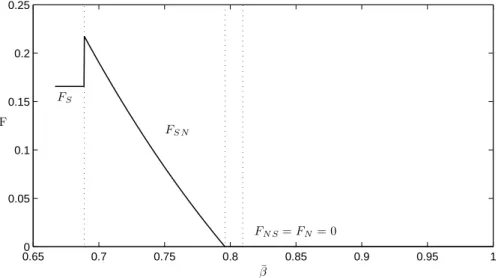
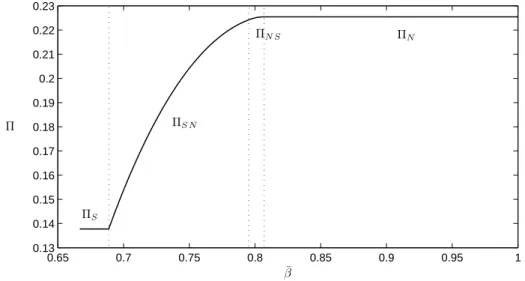
4.3 The impact of na¨ıvet´e on the optimal strategies and the profit per customer
The figures 10, 11 and 12 plot the optimal interest rate, the optimal fee and the profit per customer as a function of the index of na¨ıvet´e ¯β when β0 = 2/2.
0.65 0.7 0.75 0.8 0.85 0.9 0.95 1 1.16 1.18 1.2 1.22 1.24 1.26 1.28 ¯ β R RS N RN RN S RS
Figure 10: The optimal interest rate as a function of the index of na¨ıvet´e ¯β
0.650 0.7 0.75 0.8 0.85 0.9 0.95 1 0.05 0.1 0.15 0.2 0.25 ¯ β F FS FS N FN S=FN= 0
0.65 0.7 0.75 0.8 0.85 0.9 0.95 1 0.13 0.14 0.15 0.16 0.17 0.18 0.19 0.2 0.21 0.22 0.23 ¯ β Π ΠS ΠS N ΠN S ΠN
Figure 12: The profit per customer as a function of the index of na¨ıvet´e ¯β
5
The Impact of Competition
This section studies the impact of full competition on the equilibrium pricing strategies. We assume the following : (i) entry is unrestricted and costless, (ii) there are no capacity
constraints, and (ii) firms compete by announcing a (R, F) couple. We show that the
impact of competition depends crucially on the degree of na¨ıvet´e of the borrowers. We first study the polar cases (full na¨ıvet´e and full sophistication), then we solve the intermediate case (β0<β <¯ 1).
5.1 Fully sophisticated versus fully na¨ıves
Lets’s examine the impact of competition when the borrowers are fully sophisticated. Competition is a two dimensions game, since firms may increase their market share either
by reducing R or by increasing F. However, it is easy to show that choosing a slightly
lower interest rate than the other firms is always the dominant strategy. Suppose for
instance that there are two identical firms and let R2 > 1 and F2 > 0 be the interest
rate and the fee chosen by firm 2. Firm 1 may increase its profit by choosing any F1 >
F2, as long as (1/R2)2 < 1/(R2 +F2) (Firm 1 takes all the consumers in the interval
[1/(R2 +F1),1/(R2+F2)], which yields a net profit equal to (R−1) per consumer) 10.
But decreasing marginally the interest rate (choosing R1 = R2 −ϵ) is a much better
strategy, since it allows the firm to take the whole market (profits are multiplied by a factor slightly less than 2). Of course, the same logic applies for firm 2. Therefore the
equilibrium is such thatR1 = R2 = 1, which implies that the fees are no longer needed.
The same reasoning applies for any number of firms. Firm’s profits are null at equilibrium and all the surplus is taken by the consumers. Furthermore, time inconsistency is no
longer a problem, since borrowing at period 2 at interest rateR = 1 entails no loss from
the point of view of the period one self.
Has competition the same beneficial effects when borrowers are fully na¨ıve? Na¨ıve borrowers are not aware of the benefits and dangers of the penalty fees, since they don’t
10This applies as long as 1/(R
2+F1)≥(1/R2)2. Increasing furtherR1 leads to a loss for firm 1, due to
realize their time inconsistency problem. They, therefore, do not take into account the
fee when comparing the borrowing contracts. The only relevant variable in the (R, F)
contract is the the interest rate, which implies that the firms are free to set the fee at the level they see fit. This open the way for a new strategy based on deceit.
Suppose, for instance, that all the other firms set R = 1 (the equilibrium level when
agents are sophisticated). A positive profit can be made with the following strategy : offer
a one period contract with a “discount” interest rateR <1 and the possibility to rollover
at cost R+F 11. All agents will take the contract, and then a fraction G(1/(R+F))
will rollover (those whose preferences are such that β ≤1/(R+F)). The firm will loose
R−1 per contract on the one period borrowers (whose mass is 1−G(1/(R +F)) and
gainR(R+F)−1 per contract on the G(1/(R+F)) individuals who will rollover. The
expected profit of the firm thus writes : Π(R, F) = (R(R+F)−1)G ( 1 R+F ) + (R−1) ( 1−G ( 1 R+F )) (15)
which is positive for someR <1 andF >0 (see the end of appendix D.1). Of course, all
other firms will offer the same contract. Then free entry implies, again, that the equilibrium will be a zero-profit one. A symmetric equilibrium will therefore be characterized by the
following three conditions : (i) all firms choose the same interest rate R ; (ii) each firm
chooses the penalty fee F so as to maximize her expected profit given R ; (iii) expected
profits are null. In the appendix D.1, we show that these three conditions imply that the equilibrium (R, F) are : RcN = 1 + √ β0 2 (16) FNc = √1 β0 − 1 +√β0 2 (17)
where the superscriptc stands for competition, and the subscriptN for fully na¨ıve.
5.2 The equilibrium with partially na¨ıve agents
Recall that the agent’s population is divided in two groups : the sophisticated ones (those withβ ≥β¯) and the partially na¨ıves (those withβ <β¯). Both groups are aware of their time inconsistency problem and, therefore, do realize the commitment value of the fee. The big difference between the two groups is that the partially na¨ıve can be fooled by an appropriate contracts, whereas the sophisticated cannot.
The deceitful contract has the same structure as before : a one period lending contract
with a “discount” interest rateR <1, and the possibility to rollover at cost R+F. The
key condition is thatR andF must verify :
¯
β ≥ 1
R+F (18)
Condition (18) implies that nobody expect to roll-over, since the expected discount factor is ˜β(β) ≥ β¯ ≥ 1/(R+F). When the firms offer this kind of contract, the game is very much the same as the one played with fully na¨ıve agents. The firms are free to set the
11
The firm may also propose a portfolio of two contracts, where contract 1 is the standard contract at rateR= 1 (with costless rollover) and contract 2 is the discount contract (R <1), with a penalty F in case of rollover. The outcome will be the same, since the expected surplus from contract 1 (1−β) is lower than the expected surplus for contract 2 (1−βR) for all na¨ıves.
level of the fee, since all agents consider that the fee is big enough to deter rollover (and nobody expects to pay the fee). Therefore firms compete by offering the lowest interest rate. Free entry implies a zero-profit equilibrium.
A symmetric equilibrium will therefore be characterized by the following three
condi-tions : (i) all firms choose the same interest rateR ; (ii) each firm chooses the penalty fee
F so as to maximize her expected profit givenR subject to condition (18); (iii) expected
profits are null. It is easy to show (see appendix D.2) that there are two equilibrium configuration.
The constrained equilibrium arises when the share of partially na¨ıve agents is low ( ¯β < √β0). F is such that all the partially na¨ıve rollover R+F = 1/β¯. Then, the zero
profit condition yields :
RcP N = ¯ β¯(1−β0) β(1−β0) + (1−β¯)( ¯β−β0) (19) FP Nc = 1¯ β − ¯ β(1−β0) ¯ β(1−β0) + (1−β¯)( ¯β−β0) (20)
where the subscriptP N stands for partially na¨ıve.
The unconstrained equilibrium arises when the share of partially na¨ıve agents is high
( ¯β ≥√β0). The firms make the same choice as in the fully na¨ıve case. Therefore :
RcP N = RcN (21) FP Nc = √1 β0 − RcN ≡FNc (22) andRc P N+FP Nc = 1/ √
β0 >1/β¯. Figures (13) and (14) show the equilibriumF andRas a
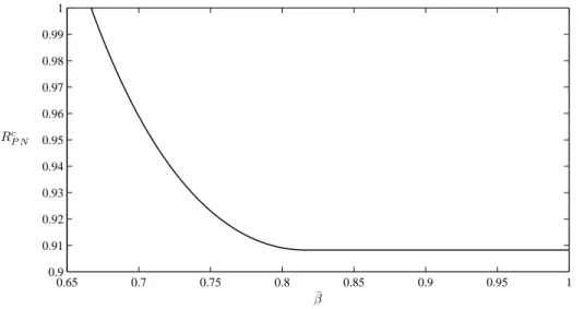
function of the index of na¨ıvet´e ¯β. Both the fee and the interest rate decrease with ¯β (this is a general result,∂RcP N/∂β <¯ 0 and∂FP Nc /∂β <¯ 0,∀β¯∈]β0,1]). Incumbent firms react
to the increase of the share of the na¨ıvesG( ¯β), by cutting the penalty feeF, which reduces the profit par na¨ıve customer but increases the market share of the exploitative contracts.
The latter effect dominates as long as 1/(R+F) ≤ √β0 (recall that R+F = 1/√β0
maximizes the expected profit for fully na¨ıve borrowers). Positive profits lead to the entry of new firms, which brings down the interest rate.
Note that the pricing policy engenders a cross-subsidy from the na¨ıves to the
so-phisticated individuals (and some of the na¨ıves too when ¯β ≥ √β0). Each one of the
G(1/(R+F)) na¨ıves that roll-over “pays”R(R+F)−1 to the 1−G(1/(R+F)) individuals that manage to stick to the one period loan. Note also that, somewhat counterintuitively, the intensity of exploitation (as measured by the penalty fee) is globally decreasing with the index of na¨ıvet´e, and is maximal when the share of na¨ıves id close to zero.
0.65 0.7 0.75 0.8 0.85 0.9 0.95 1 0.9 0.91 0.92 0.93 0.94 0.95 0.96 0.97 0.98 0.99 1 Rc P N ¯ β
Figure 13: The equilibrium interest rate under competition as a function of the index of na¨ıvet´e ¯β 0.65 0.7 0.75 0.8 0.85 0.9 0.95 1 0.32 0.34 0.36 0.38 0.4 0.42 0.44 0.46 0.48 0.5 Fc P N ¯ β
Figure 14: The equilibrium fee under competition as a function of the index of na¨ıvet´e ¯β
6
A Welfare Analysis
6.1 A paternalistic approach
Evaluating the borrower’s welfare is difficult since preferences are time-varying. One solution, proposed by O’Donoghue and Rabin (1999a,b), is to distinguish between the long-run welfare and the actual welfare. Note that the intertemporal utility of the agent can be rewritten as : ut+β ∑ s≥t+1 δs−tu s= (1−β)ut+βVtLR (23) whereVtLR =∑
s≥tδs−tus stands as the long run utility of the agent. With this formula-tion the actual intertemporal utility of the individual is an average of his short-run utility
(ut) and his long-run utility (VtLR). Rabin asserts that VtLR, which is time-consistent, is the relevant measure of the agent’s welfare.
WithVLR
t as the welfare index any type of borrowing is harmful in a monopoly setting
since R > 1 (recall that δ = 1 and ut is linear). In this sense all contracts that lead
some agents to borrow either for one period or two periods are exploitative in a monopoly setting. The aggregate welfare losses are just equal to the monopoly profits, which are an
increasing function of the index of na¨ıvet´e ¯β (this is due to the fact that the net global
surplus is equal to zero). However the individual losses depend on a non trivial way on the borrower’s impatienceβ and na¨ıvet´e ˜β(β). When all the individuals are sophisticated,
the more impatient (those who take a two-period loan) loose 1−(RS)2 each, whereas the
patient borrowers (those who take a one-period loan) loose 1−RS each 12. When all the
individuals are na¨ıves, all those who borrow take a two-period loan which leads to a loss equal to 1−(RN)2. This loss is clearly greater that the losses incurred by any sophisticated borrower, weather patient or impatient, sinceRN > RS. Yet the partially na¨ıves may loose more than the fully na¨ıves. The patient ones (those who borrow for one period) pay a
higher interest rate (RSN > RN), and the impatient ones end up paying a two-period loan
plus a penalty fee, which leads to a loss equal to 1−RSN(RSN +FSN)<1−(RN)2 (her loss is greater than the loss sustained by a fully na¨ıve that take a two-period loan). Partial na¨ıvet´e is therefore worse than full na¨ıvet´e for those who borrow.
Perfect competition drives the profits to zero. This has a positive impact on the average borrower’s welfare, which is now equal to zero (recall that the net global surplus is zero). However the impact of competition on individuals crucially depends on their na¨ıvet´e. Sophisticated individuals (those who manage to borrow for one period) can’t
loose from competition. When everybody is sophisticated ( ¯β = β0), the interest rate is
R = 1, which implies that all individuals have a surplus equal to zero. When some of
the individuals are na¨ıve, the sophisticated earn a positive surplus since R < 1. Note
that this surplus rises with the index of na¨ıvet´e ¯β (since R is a decreasing function of
¯
β). The gains of the sophisticated are the losses of the na¨ıves (those who borrow for two
periods and therefore pay the penalty fee). It must be noted that the losses of the na¨ıves
1−R(R+F) are, generally, lower under competition. Let’s show this when all individuals
are fully na¨ıve. Under monopoly, all individuals in the [β0,1/RN] interval borrow for one period and then rollover, which lead to a loss equal to 1−(RN)2 (there is no penalty fee). Under perfect competition, the same applies for all the individuals in the [β0,√β0] interval,
which lead to a loss equal to 1−Rc
N(RcN +FNc). The welfare loss under competition is lower since RcN(RNc +FNc) = RcN/√β0 < 1/√β0 < RN < (RN)2. Yet some na¨ıves are made worse off by competition : those who do not borrow under monopoly (those whose
β ∈]1/RN,√β0]). Figure 15 show the extent of two period borrowing under monopoly
and perfect competition.
12
Note that there is always a fraction a of the potential borrowers (the very patient) that choose to abstain from borrowing.
1 β0 1-period Contract β + Roll-over β0 1-period Contract + Roll-over 1-period Contract Monopoly Perfect Competition 1/RN
Figure 15: Exploitative contracts under monopoly and perfect competition with fully na¨ıve agents
The same logic applies under partial na¨ıvet´e. The na¨ıves that roll-over under monopoly and competition benefit from competition, since they pay lower rates (including the penalty fee). But the na¨ıves who do not borrow under monopoly are made worse-off by competi-tion. 13
6.2 Welfare from the point of view of self one
Using the long run utility as a measure of welfare has one big drawback : it may lead to violate the individual’s choice at each point of time. This certainly can be considered as hard paternalism. Sunstein and Thaler (2003) preconize a softer approach, which they call
libertarian paternalism14. The purpose of libertarian paternalism is to help the individual
to make freely the “right” choices. This implies that another welfare measure must be chosen. Utility at time one seems to be the natural choice, since it represents the wills of at least one of the multiple selves of the individual and is not too far from the long-run
utility 15. Note that the credit market is no longer useless, as it fulfills the “legitimate”
need for credit of self one. Lending for one period creates a surplus equal to 1−δ, which
is shared between the bank and the borrower.
Sophisticated agents cannot loose from borrowing. Their need for commitment devices is partially fulfilled under monopoly (they would prefer a higher penalty fee), and entirely fulfilled under competition (since the optimal contract deters them from renewing the loan). Competition clearly benefits them since they take the whole surplus of the exchange (plus a transfer from the na¨ıves).
Na¨ıves may loose from borrowing under monopoly, since they over-estimate the benefits of the loan. For instance when all the borrowers are fully na¨ıve, of all the individuals who
borrow and then roll-over the loan, all those whose β ∈](1/RN)2,1/RN] have a welfare
loss. This is no longer the case under perfect competition. The individuals that roll-over
the loan have a welfare gain equal to 1−βRc
N(RcN +FNc) = 1−βRcN/
√
β0 > 0 (since
β <√β0). In fact all na¨ıves are made better off by competition, even those who do not
13
There are in fact two cases. When the index of na¨ıvet´e is low ( ¯β≤√β0), the same population borrows
and roll-over under monopoly and competition (those whoseβ ∈[β0,β¯]). Therefore nobody looses from
competition. When the index of na¨ıvet´e is high ( ¯β > √β0), a fraction of the individuals that borrow
and roll-over under competition do not so under monopoly (those whoseβ ∈]1/RN,√β0]). This is the
population that looses from competition.
14
Camerer et al. (2003) use the term “asymmetric paternalism”, others prefer the slightly ironic “soft paternalism”.
15We mean, of course, self one real utility (the one he will derive by his effective consumption path), as
roll-over under monopoly16. These results extend to the partially na¨ıve case17.
7
Conclusion
This paper studies the equilibrium predatory practices that may arise when the bor-rowers have behavioral weaknesses. Rational lenders offer short term contracts that can be renewed at the cost of paying a penalty fee. We show how the optimal contracts depend on the degree of na¨ıvet´e of the time inconsistent customers. Penalty fees have a dual role : they increase market share by providing a useful commitment device to time-inconsistent but otherwise rational borrowers ; they are also a source of revenue from the semi-na¨ıve borrowers who understand the need for commitment but fail to forecast their future time discount factor. We also show that perfect competition does not eliminate predatory prac-tices, since the equilibrium contract entails a subsidized (below marginal cost) short-term loan that can only be profitable if a fraction of the borrowers end up paying the penalty fee.
References
Agarwal, S., P. Skiba, and J. Tobacman (2009). Payday loans and credit cards: New
liquidity and credit scoring puzzles? N.B.E.R. 14659.
Ausubel, L. (1991). The failure of competition in the credit card market. The American
Economic Review, 50–81.
Camerer, C., S. Issacharoff, G. Loewenstein, T. O’Donogue, and M. Rabin (2003, April). Regulation for conservatives: Behavioral economics and the case for asymmetric
pater-nalism. University of Pennsylvania Law review 151, 1211–1254.
Della Vigna, S. and U. Malmendier (2004, May). Contract design and self-control: Theory
and evidence. The Quarterly Journal of Economics 119(2), 353–402.
Della Vigna, S. and U. Malmendier (2006, June). Paying not to go to the gym. 96(3),
694–719.
Eliaz, K. and R. Spiegler (2006). Contracting with diversely naive agents. 73, 689 ˝U714.
Gabaix, X. and D. Laibson (2006). Shrouded Attributes, Consumer Myopia, and
Infor-mation Suppression in Competitive Markets. Quarterly Journal of Economics 121(2),
505–540.
Gottlieb, D. (2008, August). Competition over Time-Inconsistent consumers. Journal of
Public Economic Theory 10(4), 673–684.
Heidhues, P. and B. K˝oszegi (2009). Futile attempts at self-control. Journal of the
Euro-pean Economic Association 7(2-3), 423–434.
16
Proof. The welfare gain for the fully na¨ıve is, under monopoly : 1−β(RN)2 if β < 1/RN and 0
if β ≥ 1/RN; and under perfect competition 1−βRcN/
√
β0 if β < √β0, and 1−βRcN if β ≥
√
β0.
1/RN < √β0, therefore we have three cases: (i) β ∈ [β0,1/RN[, 1−β(RN)2 < 1−βRcN/
√β
0 since
RN >1/√β0 > 1 > RcN; (ii) β ∈ [1/RN,√β0[,0 < 1−βRcN/
√β
0, since β < √β0 and RcN < 1; (iii)
β∈[√β0,1],0<1−βRcN, sinceRcN<1. 17Proof. If ¯β
Heidhues, P. and B. K˝oszegi (2010). Exploiting naivete about self-control in the credit
market. 100(5), 2279–2303.
Laibson, D. (1997). Golden eggs and hyperbolic discounting. Quarterly Journal of
Eco-nomics 112(2), 443–477.
O’Donoghue, T. and M. Rabin (1999a). Doing it now or later. 89, 103–24.
O’Donoghue, T. and M. Rabin (1999b). Incentives for procrastinators. 114, 769–816.
O’Donoghue, T. and M. Rabin (2001). Choice and procrastination. 116, 121–160.
O’Donoghue, T. and M. Rabin (2003). Studying optimal paternalism, illustrated by a
model of sin taxes. 93(2), 186–191.
O’Donoghue, T. and M. Rabin (2006). Optimal sin taxes.Journal of Public Economics 90,
1825–1849.
Shui, H. and L. Asubel (1995). Time inconsistency in the credit card market. Working
Paper, Department of Economics, University of Maryland.
Stegman, M. (2007). Payday lending. Journal of Economic Perspectives 21(1), 169–190.
Sunstein, C. and R. Thaler (2003). Libertarian paternalism is not an oxymoron. The
University of Chicago Law Review 70(4), 1159–1202.
A
Sophisticated borrowers
A.1 The profit function when F ≥ β1 0 −
√
1
β0
In this case, the profit function writes :
Π(R, F) = { (R2−1)G(R+1F)+ (R−1)[G(1 R ) −G(R+1F)] if 1≤R<1 β0−F (R−1)G(1 R ) if 1 β0−F≤R≤ 1 β0 (24)
Proof. All individuals choose one-period contract when 1/β0 −F ≤ R ≤ 1/β0, since
they are profitable (βR < 1, ∀β) and the individuals know that they will not rollover
(β(R +F) > 1, ∀β). The profit is therefore (R −1) times the number of contracts
G(1/R). R < 1/β0 −F < 1/√β0 imply that β0 < 1/(R+F) < 1/R2 < 1/R (recall
thatF ≥1/β0−
√
1/β0 =⇒ RF ≥√β0). From this we know that : (i) some individuals
will roll-over (those such that β < 1/(R +F)); (ii) 2-period contracts are profitable
for those individuals (since 1/(R+F) < 1/R2). All the other individuals choose
one-period contracts. The profit is therefore (R2−1) times the number of 2-period contracts
G(1/(R+F)) plus (R−1) times the number of one-period contractsG(1/R)−G(1/(R+F)).
Let’s show that the optimalF cannot be greater than β10 −√β10.
First we show that the interest rate R∗ that maximizes Π(R, F) (for a given F ≥
1/β0 −
√
1/β0) lies in the interval ]1,1/√β0]. Let’s assume that R∗ > 1/β0 −F. The
profit function then writes Π(R, F) = (R −1)G(1/R) = Π1(R). The first and second
derivative of Π1(R) are : Π′ 1(R) = 1 β0 ( 1 R −β0−1 + 1 R2 ) Π′′1(R) = −1 β0 ( 1 R2 + 2 R3 )
Π′′
1(R) <0 implies that Π1(R) has a unique maximum and Π′1(1/
√ β0) = √ β0−1 β0−1 <0 =⇒ R∗ <1/√β 0.
R∗<1/√β0 implies that 1/(R∗+F)<(1/R∗)2 (sinceR
F >1/√β0). Such a
configu-ration can’t be optimal since the profit can be increased byreducing F (which allows the
firm to replace one-period contracts by the 2-period ones). This shows that the optimal
F is such that F <1/β0−
√
1/β0.
A.2 The optimum
Taking into account that the optimal F is such that F =RF(RF −1), we can write
the profit function as : ΠS(F) = (R2F −1 ) G ( 1 R2 F ) + (RF −1) ( G ( 1 RF ) −G ( 1 RF +F )) = RF(RF −1)G ( 1 R2 F ) + (RF −1)G ( 1 RF ) = 1 1−β0 ( F × ( 1 R2 F −β0 ) + (RF −1) ( 1 RF − β0 )) UsingR′ F = dRdFF = 1
2RF−1 and F =RF(RF −1) we compute the first and second
deriva-tives : Π′S(F) = 1 1−β0 ( 1 R2F −β0−2F R′ F R3F + R′ F R2F −β0R ′ F ) = 2 1−β0 × R2 F −β0R4F −F R3 F(2RF −1) = 2 1−β0 × 1−β0R3F R2F(2RF −1) Π′′S(F) = 2R′F 1−β0 × β0R3F −6RF + 2 R3 F(2RF −1)2 = − 2 1−β0 × 3 R3 F(2RF −1)2 <0 Since Π′′
S(F)<0 the maximum of the function ΠS is attained when Π′S(F) = 0 ⇔ RF =
(1/β0)1/3.
B
Fully na¨ıve borrowers
Since FN = 0,RN is the maximum of the function :
ΠN = Π(R,0) = (R2−1)G(1/R) =
(R2−1)(1/R−β0)
1−β0
in the interval [1,1/β0]. The function ΠN(R) is concave (since Π′′N(R) =−2β0+1/R
3
1−β0 ). The
maximum is the solution of
Π′N(R) = 1 1−β0 ( 1−2β0R+ 1 R2 ) = 0
which yields a cubic equation (−2β0R3+R2+1 = 0). Since Π′N(1) = 2>0 and Π′N(1/β0) =
−(1 +β0)<0, this equation has a unique solution in the interval [1,1/β0].
Π′
N(1/
√
C
Partially Na¨ıve borrowers
C.1 The profit function
For the sake of simplicity we write the profit function as a function ofRandZ =R+F.
There are five different regions (see figures 16 and 17 for a mapping in the (R, Z) space).
Hereupon we show that the profit function writes, whenβ0<β <¯ √β0 (figure 16 and 17)
Π(R, Z) = Π1(R,Z)≡(R−1)G(R1) if Z≥β1 0 and R≤Z Π2(R,Z)≡R(Z−1)G(Z1)+(R−1)G(R1) if 1β¯≤Z< 1 β0 and R≤Z Π3(R,Z)≡(R−1)[G(R1)−G(Z1)] if Z<β1¯ and 1 √β 0≤R≤Z Π4(R,Z)≡(R2−1)G ( 1 R2 ) +(R−1)[G(1 R)−G( 1 Z)] if Z< 1 ¯ β and √ Z≤R<max { Z, 1 √ β0 } Π5(R,Z)≡R(R−1)G(Z1)+(R−1)G(R1) if Z<β1¯ and R< √ Z (25) and, forβ0 <√β0 ≤β¯(figure 18):
Π(R, Z) = Π1(R,Z)≡(R−1)G(R1) if Z≥β1 0 and R≤Z Π2(R,Z)≡R(Z−1)G(Z1)+(R−1)G(R1) if β1¯≤Z<β1 0 and R≤Z Π4(R,Z)≡(R2−1)G ( 1 R2 ) +(R−1)[G(1 R)−G( 1 Z)] if Z< 1 ¯ β and √ Z≤R≤Z Π5(R,Z)≡R(R−1)G(Z1)+(R−1)G(R1) if Z<1β¯ and R< √ Z (26) Proof: Region 1: Z ≥ β1 0 and R≤Z =⇒ 1/Z ≤β0 < ¯
β <1/R. All individuals choose the one period contract, since they don’t expect to rollover ( ˜β(β) ≥ β >¯ 1/Z,∀β). No one rollovers sinceβ ≥β0>1/Z. The profit is (R−1) times the number of contractsG(1/R).
Region 2: 1β¯ ≤ Z < β10 and R ≤ Z =⇒ β0 < 1/Z ≤ β <¯ 1/R. As before all
individuals choose the one period contract. But some individuals will rollover (those with
β <1/Z). The profit is (R−1) times the number of one period contractsG(1/R)−G(1/Z)
plusRZ−1 times the number of individual who rollover G(1/Z).
Region 3: Z < β1¯ and √1
β0 ≤R ≤Z =⇒ 1/R
2 ≤β
0 <β <¯ 1/Z <1/R. All
individ-uals withβ >1/Z choose (rightly) the one period contracts since ˜β(β) =β >1/Z,∀β >
1/Z. All the other individuals expect to rollover, and thus abstain from borrowing
(two-period contracts are not profitable sinceβ > 1/R2,∀β). The profit is (R−1) times the
number of one period contractsG(1/R)−G(1/Z).
Region 4: Z < β1¯ and √Z < R <max{Z,√1
β0
}
=⇒ β0 < max{β,¯ 1/R2} ≤1/Z <
1/R. Same logic as in the previous case. All the individuals withβ <1/Z rightly expects
to rollover. They either abstain from borrowing or choose a two period contract (which
is profitable for those with β < 1/R2). The profit is (R−1) times the number of one
period contractsG(1/R)−G(1/Z) plusR2−1 times the number of two period contracts
G(1/R2).
Region 5: Z < β1¯ and R≤√Z =⇒ β0 <β <¯ 1/Z <1/R2 <1/R. Same logic as in
the previous case. All the individuals with β <1/Z choose a two period contract. The
profit is (R−1) times the number of one period contractsG(1/R)−G(1/Z) plusR2−1
C.2 The profit maximizing strategy when the borrowers are partially na¨ıve
It is easy to see that the profit function is not convex, and has several discontinuities (the profit jumps between region 2,3 and 4 and between region 2 and region 5). Our method is first to compute the sign of the partial derivatives in each region in order to locate the local maxima, and then compare those maxima. The arrows in figures 16, 17 and 18 show the “directions” that the firm must follow to increase her profit.
We distinguish three cases.
Case 1: β0≤β <¯ √β0 and RSN = √ ¯ β β0−β¯(1−β¯) < 1 ¯ β The optimum profit strategy are :
(S) R=(β1 0 )1/3 ≡RS and Z = ( 1 β0 )2/3 if β0 ≤β <¯ β¯1 (SN) R=√β β¯ 0−β¯(1−β¯) ≡RSN and Z = 1/ ¯ β if β¯1 ≤β <¯ β¯2
where ¯β1 <β¯2 <1 are given at the end of the subsection.
Proof.
First we show that the optimal strategy in this configuration must be either (S) or
(SN) (see figure 16). Let’s begin with region 1. The profit function does not depends on
Z. The derivative with respect toR is :
(1−β0) ∂Π1(R, Z) ∂R = 1 R2 −β0 (< > ) 0 if R(> < ) 1 √ β0
The local maximum is therefore attained whenR= 1/√β0 (∀Z ≥1/β0). But the global
optimum cannot lie in region 1 since Π2(R, Z)−Π1(R, Z) = (RZ−1)G(1/Z)>0∀Z >1.
Let’s move to region 2. The partial derivatives of the profit function are : (1−β0) ∂Π2(R, Z) ∂Z = R ( 1 Z2 −β0 ) <0 since Z > 1¯ β > 1 √ β0 (1−β0) ∂Π2(R, Z) ∂R = (Z−1) ( 1 Z −β0 ) + 1 R2 −β0 (< = > ) 0 if R(=> < ) ϕ(Z) whereϕ(Z) =√1−Z(1Z−β
0Z) is a continuous function that crosses the frontier with region
3 inR=RSN and the frontier with region 1 inR= 1/√β0.
Since∂Π2/∂Z <0, the local maximum lies in the western frontier of region 2 (Z = 1/β¯)
18, whereas the sign of ∂Π
2/∂R implies that the optimal interest rate is RSN =ϕ(1/β¯) (see figure 16).
Now we examine region 3. The partial derivatives are : (1−β0) ∂Π3(R, Z) ∂Z = R−1 Z2 >0 (1−β0) ∂Π3(R, Z) ∂R = 1 R2 − 1 Z <0 since R > √ Z
18The local maximum can’t lie in the lineR=Z since∂Π
R and Z are therefore pushed toward the frontiers with region 4 and 2 (see figure 16). Note that the profit function jumps upward when the frontier between region 3 and region 2 is crossed, since : Π2(R,1/β¯)−Π3(R,1/β¯) = ¯ β−β0 1−β0 ( R ¯ β −1 ) >0
This implies that the optimum can’t lie in region 3.
Now let’s examine region 4 and 5. The partial derivatives are : (1−β0) ∂Π4(R, Z) ∂Z = R−1 Z2 >0 (1−β0)∂Π4(R, Z) ∂R = 2 ( 1 R3 −β0 ) + 1 R2 − 1 Z (< > ) 0 if Z(< > ) ψ(R) (1−β0)∂Π5(R, Z) ∂Z = − R(R−1) Z2 <0 (1−β0) ∂Π5(R, Z) ∂R = (2R−1) ( 1 Z −β0 ) + 1 R2 − 1 Z >0 since R≤ √ Z whereψ(R) =( 2( 1 R3 −β0 ) +R12 )−1
is an increasing function ofR which cross theR=Z
line in Z = Z1 ∈]1,(1/β0)2/3[ and the frontier between region 4 and 5 in R = (1/β0)1/3
andZ = (1/β0)2/3.
The sign of the derivatives imply that the local maximum lies in the frontier between region 4 and 5. It is easy to check that the local optimum is such that : R= (1/β0)1/3 =RS andZ = (1/β0)2/3=ZS (see figure 16) 19.
Now we show that strategy (S) is chosen for low ¯β whereas strategy (SN) is optimal
otherwise. Let’s compute the optimal profit for both strategies : ΠS = Π4(RS, ZS) = 1−β01/3 1−β0 ( 2−β01/3−β02/3) ΠSN = Π2(RSN, ZSN) = 1 1−β0 ( 1 +β0− 2 RSN ) Thus ΠS >ΠSN when : RSN = √ ¯ β β0−β¯(1−β¯) > 2 3β01/3−1 which is verified for all ¯β∈[β0,β¯1[, where ¯β1 = −b−
√
b2−4ac
2 (witha= 1,b=−(1+(3β
1/3 0 −
1)2/4) and c=β0) is the unique positive solution of the equation :
¯ β2− ( 1 +1 4 ( 3β10/3−1)2 ) ¯ β+β0 = 0
Now we compute the upper bound ¯β2. The strategy (SN) is chosen when ¯β≥β¯1 and :
RSN ≤ZSN = 1/β¯ ⇐⇒ √ ¯ β β0−β¯(1−β¯) ≤ 1/β¯ ¯
β2 therefore solves the following cubic equation :
Υ( ¯β) = ¯β3−β¯2+ ¯β−β0= 0
It is easy to check that equation Υ( ¯β) = 0 has a unique solution in the interval [β1,1]. 20
19
The optimum strategy isRS= argmax Π4(R, R2) andZS=R2. 20 Υ(β0) =β 2 0(β0−1)<0, Υ(1) = 1−β0>0 and Υ′( ¯β) = 3 ¯β 2 −2 ¯β+ 1>0,∀β¯∈[β0,1]
Case 2: β0≤β <¯ √β0, RSN = √ ¯ β β0−β¯(1−β¯) ≥ 1 ¯ β and RN <1/β¯ The optimum profit strategy is :
(NS) R= 1/β¯=RN S and Z = 1/β¯=ZN S for β¯2 ≤β <¯ β¯3
where ¯β3 is given at the end of the subsection.
Proof.
As before (see figure 17) there is a local optimum at the frontier between region 4 and
5 (R=RS and Z =ZS). We shall prove that this optimum can’t be the global one
The other local optimum lies either at the western frontier or at the northern frontier
of region 2 (since∂Π2/∂Z < 0). The profit maximizing strategy at the western frontier
(the one such that Z = 1/β¯) is R = Z = 1/β¯ since ∂Π2(R,1/β¯)/∂R > 0. This
strat-egy is also the profit maximizing stratstrat-egy at the northern frontier since RN < 1/β¯ ⇒
dΠ2(R, R)/dR <0∀R≥1/β¯. 21
Therefore ¯β3 = 1/RN (sinceR=Z = 1/β¯is no longer the profit maximizing strategy
whenRN ≥1/β¯).
Let’s show that the (NS) strategy is better than the (S) strategy when ¯β ∈ [ ¯β2,β¯3[.
The profit of the (NS) strategy writes :
ΠN S = Π2(1/β,¯ 1/β¯)= ¯ β−β0 1−β0 ( 1 ¯ β2 −1 ) Therefore : dΠN S dR = 1 1−β0 ( −¯1 β2 + 2 β0 ¯ β3 −1 )
It is easy to show thatdΠN S/dβ >¯ 0 if ¯β2 ≤β <¯ 1/RN 22. This and ΠN S = ΠSN >ΠS for ¯β= ¯β2 imply that ΠN S >ΠS ∀β¯∈[ ¯β2,β¯3[.
Case 3: RN ≥1/β¯ 23
The optimum profit strategy is :
(N) R=RN and Z =ZN for β¯3 ≤β¯≤1
Proof.
As seen in figure 18, there is a local optimum at the frontier between region 4 and 5
and another at the northern frontier of region 2 (sincedΠ2/dR >0). The profit function
in the latter case writes:
ΠN = Π2(R, R) =(R2−1)G(1/R2)
which is also the profit when the agents are fully na¨ıve. The unique maximum of ΠN is
attained whendΠN/dR= 0 ⇔ R=RN (see section B for the full proof).
21
Recall thatRN is the profit maximizing strategy for fully na¨ıve agents. 22
Let dΠN S/dβ¯= Ω( ¯β). Simple algebra yields Ω( ¯β2) = − ¯ β2 2−β0 1−β0 >0 (since ¯β < √ β0) and Ω( ¯β3) = 0 (since ¯β3= 1/RN and−2β0RN3 +R 2
N+ 1 = 0). This and the fact that ¯β3 is the only solution of the the
equation Ω( ¯β) = 0 in the interval [β0,1] implies that Ω( ¯β)>0,∀β¯∈[ ¯β2,β¯3[ 23
There a two sub-cases : case 3.a (such that ¯β <√β0 andRN>1/β¯) and case 3.b ( ¯β≥√β0⇒RN >
The (N) strategy is always better than the (S) strategy since ΠN ≥ΠN S >ΠSN >ΠS. Π1 Π1 Π2 Π4 Π5 Π2 β0 1/ β_ 1/ _ 1/β 1/β0 (1/β0) 1/2 Π3 R=Z1/2 R Z 1 1 R=Z S SN RS RSN
Π1 Π1 Π2 Π4 Π5 Π2 β0 1/ β_ 1/ _ 1/β 1/β0 (1/β0) 1/2 Π3 R=Z1/2 R Z 1 1 R=Z S NS RS RNS= RN
Figure 17: A mapping of the profit function when β0 < β <¯ √β0, RSN ≥ 1/β¯ and
RN <1/β¯ Π1 Π1 Π2 Π4 Π5 Π2 β0 1/ β _ 1/ _ 1/β 1/β0 (1/β0) 1/2 R=Z1/2 R Z 1 1 R=Z S RS RN N (1/β0) 1/2 Π2
D
The impact of competition
D.1 Fully na¨ıve borrowers
The equilibrium is such that : (i) all firms choose the sameR; (ii) each firm choosesF
so as to maximize her expected profit givenR ; (iii) expected profits are null. Assuming
that there is a continuum of firms of sizem(the variablemis unimportant), condition (ii)
implies : F∗(R) = arg max F Πi(R, F) = 1 m [ (R(R+F −1)G ( 1 R+F ) + (R−1) ]
where Πi(R, F), the profit of firmi, is a concave function ofF. Thus :
∂Πi(R, F) ∂F = 1 m R 1−β0 ( 1 (R+F)2 −β0 ) = 0 =⇒ F∗(R) = √1 β0 − R
The zero profit condition (iii) then writes : Πi(R, F∗(R)) = 1 m [ 2R 1 +√β0 − 1 ] = 0 which yieldRcN = (1 +√β0)/2 and FNc =F∗(RcN).
We use these calculations to show that the expected profit of a firm that choosesR <1
and F >0 when all other firms choose R= 1 is positive for some F. LetR = 1−ϵand
F∗(1−ϵ) be the interest rate and the fee chosen by the firm. Her profit writes :
Πi(1−ϵ, F∗(1−ϵ)) = [ 2(1−ϵ) 1 +√β0 − 1 ] which is positive∀ ϵ <(1−√β0)/2.
D.2 Partially na¨ıve borrowers
The fee is chosen so as to maximize the expected profit per consumer subject to con-dition (18) : F∗∗(R) = arg max F Πi(R, F) = 1 m [ (R(R+F −1)G ( 1 R+F ) + (R−1) ] s.t. R+F ≥1/β¯
This program has two solutions : constrained and unconstrained. The unconstrained solution is the one given in appendix D.1. It arises whenR+F∗ = 1/√β0 ≥1/β¯.
The constrained solution is such that : R+F∗∗ = 1/β¯ and ∂Π
∂F < 0 (which is a
consequence ofR+F∗∗= 1/√β0 <1/β¯). Then the profit writes :
Πi(R, F∗∗(R)) =R ( 1 ¯ β −1 ) ¯ β−β0 1−β0 +R−1
The zero profit condition Πi(R, F∗∗(R)) = 0 yield the equilibrium valueRcP N and FP Nc = 1/β¯−RP Nc .