Benchmarking Least Squares Support Vector
Machine Classifiers
TONY VAN GESTEL [email protected]
JOHAN A.K. SUYKENS [email protected]
Department of Electrical Engineering, ESAT/SISTA, Katholieke Universiteit Leuven, Belgium
BART BAESENS [email protected]
STIJN VIAENE [email protected]
JAN VANTHIENEN [email protected]
GUIDO DEDENE [email protected]
Leuven Institute for Research on Information Systems, Katholieke Universiteit Leuven, Belgium
BART DE MOOR [email protected]
JOOS VANDEWALLE [email protected]
Department of Electrical Engineering, ESAT/SISTA, Katholieke Universiteit Leuven, Belgium
Editor:Peter Bartlett
Abstract. In Support Vector Machines (SVMs), the solution of the classification problem is characterized by
a (convex) quadratic programming (QP) problem. In a modified version of SVMs, called Least Squares SVM classifiers (LS-SVMs), a least squares cost function is proposed so as to obtain a linear set of equations in the dual space. While the SVM classifier has a large margin interpretation, the LS-SVM formulation is related in this paper to a ridge regression approach for classification with binary targets and to Fisher’s linear discriminant analysis in the feature space. Multiclass categorization problems are represented by a set of binary classifiers using different output coding schemes. While regularization is used to control the effective number of parameters of the LS-SVM classifier, the sparseness property of SVMs is lost due to the choice of the 2-norm. Sparse-ness can be imposed in a second stage by gradually pruning the support value spectrum and optimizing the hyperparameters during the sparse approximation procedure. In this paper, twenty public domain benchmark datasets are used to evaluate the test set performance of LS-SVM classifiers with linear, polynomial and ra-dial basis function (RBF) kernels. Both the SVM and LS-SVM classifier with RBF kernel in combination with standard cross-validation procedures for hyperparameter selection achieve comparable test set performances. These SVM and LS-SVM performances are consistently very good when compared to a variety of methods de-scribed in the literature including decision tree based algorithms, statistical algorithms and instance based learning methods. We show on ten UCI datasets that the LS-SVM sparse approximation procedure can be successfully applied.
Keywords: least squares support vector machines, multiclass support vector machines, sparse approximation
1. Introduction
Recently, Support Vector Machines (SVMs) have been introduced by Vapnik (Boser, Guyon, & Vapnik, 1992; Vapnik, 1995) for solving classification and nonlinear function estimation
problems (Cristianini & Shawe-Taylor, 2000; Sch¨olkopf et al., 1997; Sch¨olkopf, Burges, & Smola, 1998; Smola, Sch¨olkopf, & M¨uller, 1998; Smola, 1999; Suykens & Vandewalle, 1998; Vapnik, 1995, 1998a, 1998b). Within this new approach the training problem is reformulated and represented in such a way so as to obtain a (convex) quadratic programming (QP) problem. The solution to this QP problem is global and unique. In SVMs, it is possible to choose several types of kernel functions including linear, polynomial, RBFs, MLPs with one hidden layer and splines, as long as the Mercer condition is satisfied. Furthermore, bounds on the generalization error are available from statistical learning theory (Cristianini & Shawe-Taylor, 2000; Smola, 1999; Vapnik, 1998a, 1998b), which are expressed in terms of the VC (Vapnik-Chervonenkis) dimension. An upper bound on this VC dimension can be computed by solving another QP problem. Despite the nice properties of SVMs, there are still a number of drawbacks concerning the selection of hyperparameters and the fact that the size of the matrix involved in the QP problem is directly proportional to the number of training points.
A modified version of SVM classifiers, Least Squares SVMs (LS-SVMs) classifiers, was proposed in Suykens and Vandewalle (1999b). A two-norm was taken with equal-ity instead of inequalequal-ity constraints so as to obtain a linear set of equations instead of a QP problem in the dual space. In this paper, it is shown that these modifications of the problem formulation implicitly correspond to a ridge regression formulation with binary
targets±1. In this sense, the LS-SVM formulation is related to regularization networks
(Evgeniou, Pontil, & Poggio, 2001; Smola, Sch¨olkopf, & M¨uller, 1998), Gaussian Pro-cesses regression (Williams, 1998) and to the ridge regression type of SVMs for nonlinear function estimation (Saunders, Gammerman, & Vovk, 1998; Smola, 1999), but with the inclusion of a bias term which has implications towards algorithms. The primal-dual for-mulations of the SVM framework and the equality constraints of the LS-SVM formulation allow to make extensions towards recurrent neural networks (Suykens & Vandewalle, 2000) and nonlinear optimal control (Suykens, Vandewalle, & De Moor, 2001). In this paper, the additional insight of the linear decision line in the feature space is used to relate the im-plicit LS-SVM regression approach to a regularized form of Fisher’s discriminant analysis (Bishop, 1995; Duda & Hart, 1973; Fisher, 1936) in the feature space (Baudat & Anouar, 2000; Mika et al., 1999). By applying the Mercer condition, this so-called Kernel Fisher Discriminant is obtained as the solution to a generalized eigenvalue problem (Baudat & Anouar, 2000; Mika et al., 1999).
The QP-problem of the corresponding SVM formulation is typically solved by Inte-rior Point (IP) methods (Cristianini & Shawe-Taylor, 2000; Smola, 1999), Sequential Minimal Optimization (SMO) (Platt, 1998) and iteratively reweighted least squares ap-proaches (IRWLS) (Navia-V´azquez et al., 2001), while LS-SVMs (Suykens & Vandewalle, 1999b; Suykens et al., 2002; Van Gestel et al., 2001, 2002; Viaene et al., 2001) result into a set of linear equations. Efficient iterative methods for solving large scale linear systems are available in numerical linear algebra (Golub & Van Loan, 1989). In Suykens et al. (1999) a conjugate gradient based iterative method has been developed for solving the re-lated Karush-Kuhn-Tucker system. In this paper, the algorithm is further refined in order to combine it with hyperparameter selection. A drawback of LS-SVMs is that sparseness is lost due the choice of a 2-norm. However, this can be circumvented in a second stage
by a pruning procedure which is based upon removing training points guided by the sorted support value spectrum and does not involve the computation of inverse Hessian matrices as in classical neural network pruning methods (Suykens et al., 2002). This is important in view of an equivalence between sparse approximation and SVMs as shown in Girosi (1998).
A straightforward extension of LS-SVMs to multiclass problems has been proposed in Suykens and Vandewalle (1999c), where additional outputs are taken in order to encode multiclasses as is often done in classical neural networks methodology (Bishop, 1995). This approach is different from standard multiclass SVM approaches. In Suykens and Vandewalle (1999c) the multi two-spiral benchmark problem, which is known to be hard for classical neural networks, was solved with an LS-SVM with a minimal number of bits in the class coding and yielded an excellent generalization performance. This approach is further extended here to different types of output codings for the classes, like one-versus-all, error correcting and one-versus-one codes.
In this paper, we report the performance of LS-SVMs on twenty public domain bench-mark datasets (Blake & Merz, 1998). Ten binary and ten multiclass classification problems were considered. On each dataset linear, polynomial and RBF (Radial Basis Function) kernels were trained and tested. The performances of the simple minimum output cod-ing and advanced one-versus-one codcod-ing are also compared on the multiclass problems. The LS-SVM hyperparameters were determined from a 10-fold cross-validation proce-dure by grid search in the hyperparameter space. The LS-SVM generalization ability was estimated on independent test sets in all of the cases and results of additional random-izations on all datasets are reported. In the experimental setup two third of the data was used to construct the classifier and one third was reserved for out-of-sample testing. Af-ter optimization of the hyperparameAf-ters, a very good test set performance is achieved by LS-SVMs on all twenty datasets. At this point comparisons on the same randomized datasets have been made with reference classifiers including the SVM classifier, decision tree based algorithms, statistical algorithms and instance based learning methods (Aha & Kibler, 1991; Breiman et al., 1984; Duda & Hart, 1973; Holte, 1993; John & Langley, 1995; Lim, Loh, & Shih, 2000; Ripley, 1996; Witten & Frank, 2000). In most cases SVMs and LS-SVMs with RBF kernel perform at least as good as SVM and LS-SVMs with linear kernel which means that often additional insight can be obtained whether the opti-mal decision boundary is strongly nonlinear or not. Furthermore, we successfully confirm the LS-SVM sparse approximation procedure that has been proposed in Suykens et al. (2002) on 10 UCI benchmark datasets with optimal hyperparameter determination during pruning.
This paper is organized as follows. In Section 2, we review the basic LS-SVM formulation for binary classification and relate the LS-SVM formulation to Kernel Fisher Discriminant Analysis. The multiclass categorization problem is reformulated as a set of binary classifica-tion problems in Secclassifica-tion 3. The sparse approximaclassifica-tion procedure is discussed in Secclassifica-tion 4. A conjugate gradient algorithm for large scale applications is discussed in Section 5. Section 6 elaborates on the selection of the hyperparameters with 10-fold cross-validation. Section 7 presents the empirical findings of LS-SVM classifiers achieved on 20 UCI benchmark datasets in comparison with other methods.
2. LS-SVMs for binary classification
Given a training set{(xi,yi)}iN=1with input dataxi∈IRnand corresponding binary class
la-bels yi∈ {−1,+1}, the SVM classifier, according to Vapnik’s original formulation
(Boser, Guyon, & Vapnik, 1992; Cristianini & Shawe-Taylor, 2000; Sch¨olkopf et al., 1997; Sch¨olkopf, Burges, & Smola, 1998; Smola, Sch¨olkopf, & M¨uller, 1998; Vapnik, 1995, 1998a, 1998b), satisfies the following conditions:
wTϕ(x i)+b≥ +1, if yi = +1 wTϕ(x i)+b≤ −1, if yi = −1 (1) which is equivalent to yi[wTϕ(xi)+b]≥1, i=1, . . . ,N. (2)
The nonlinear functionϕ(·):Rn→Rnhmaps the input space to a high (and possibly infinite)
dimensional feature space. In primal weight space the classifier then takes the form
y(x)=sign[wTϕ(x)+b], (3)
but, on the other hand, is never evaluated in this form. One defines the optimization problem:
min w,b,ξJ(w, ξ)= 1 2w Tw+ C N i=1 ξi (4) subject to yi[wTϕ(xi)+b]≥1−ξi, i =1, . . . ,N ξi ≥0, i =1, . . . ,N. (5)
The variablesξi are slack variables that are needed in order to allow misclassifications in
the set of inequalities (e.g., due to overlapping distributions). The positive real constant
C should be considered as a tuning parameter in the algorithm. For nonlinear SVMs, the
QP-problem and the classifier are never solved and evaluated in this form. Instead a dual space formulation and representation is obtained by applying the Mercer condition (see Cristianini & Shawe-Taylor, 2000; Sch¨olkopf et al., 1997; Sch¨olkopf, Burges, & Smola, 1998; Smola, 1999; Vapnik, 1995, 1998a, 1998b) for details.
Vapnik’s SVM classifier formulation was modified in Suykens and Vandewalle (1999b) into the following LS-SVM formulation:
min w,b,eJ(w,e)= 1 2w Tw+γ 1 2 N i=1 ei2 (6)
subject to the equality constraints
yi[wTϕ(xi)+b]=1−ei, i =1, . . . ,N. (7)
This formulation consists of equality instead of inequality constraints and takes into account a squared error with regularization term similar to ridge regression.
The solution is obtained after constructing the Lagrangian:
L(w,b,e;α)=J(w,b,e)−
N
i=1
αi{yi[wTϕ(xi)+b]−1+ei}, (8)
where αi∈IR are the Lagrange multipliers that can be positive or negative in the
LS-SVM formulation. From the conditions for optimality, one obtains the Karush-Kuhn-Tucker (KKT) system: ∂L ∂w =0→w= N i=1 αiyiϕ(xi) ∂L ∂b =0→ N i=1 αiyi =0 ∂L ∂ei =0→αi =γei, i =1, . . . ,N ∂L ∂αi =0→ yi[wTϕ(xi)+b]−1+ei=0, i =1, . . . ,N. (9)
Note that sparseness is lost which is clear from the condition αi = γei. As in standard
SVMs, we never calculatewnorϕ(xi). Therefore, we eliminatewandeyielding (Suykens
& Vandewalle, 1999b) 0 yT y +γ−1I b α = 0 1v (10) with y = [y1, . . . ,yN], 1v =[1, . . . ,1],e = [e1, . . . ,eN],α =[α1, . . . , αN]. Mercer’s
condition is applied within thematrix
i j=yiyjϕ(xi)Tϕ(xj)=yiyjK(xi,xj). (11)
For the kernel functionK(·,·) one typically has the following choices:
K(x,xi)=xiTx, (linear kernel)
K(x,xi)= 1+xiTx
cd, (polynomial kernel of degreed)
K(x,xi)=exp −x−xi 2 2 σ2, (RBF kernel) K(x,xi)=tanh κxiTx+θ , (MLP kernel),
whered,c,σ,κandθare constants. Notice that the Mercer condition holds for allc, σ ∈IR+
andd ∈ Nvalues in the polynomial and RBF case, but not for all possible choices ofκ
andθin the MLP case. The scale parametersc,σ andκdetermine the scaling of the inputs
in the polynomial, RBF and MLP kernel function. This scaling is related to the bandwidth of the kernel in statistics, where it is shown that the bandwidth is an important parameter of the generalization behavior of a kernel method (Rao, 1983). The LS-SVM classifier is then constructed as follows:
y(x)=sign N i=1 αiyiK(x,xi)+b . (12)
A simple and practical way to construct binary MLP classifiers is to use a regression
formulation (Bishop, 1995; Duda & Hart, 1973), where one uses the targets±1 to encode the
first and second class, respectively. By the use of equality constraints with targets{−1,+1},
the LS-SVM formulation (6)–(7) implicitly corresponds to a regression formulation with regularization (Bishop, 1995; Duda & Hart, 1973; Saunders, Gammerman, & Vovk, 1998;
Suykens & Vandewalle, 1999b). Indeed, by multiplying the errorei withyi ∈ {−1,+1},
the error termED=
N i=1e2i becomes ED= 1 2 N i=1 ei2= 1 2 N i=1 (yiei)2 = 1 2 N i=1 (yi−(wTϕ(xi)+b))2. (13)
Neglecting the bias term in the LS-SVM formulation, this regression interpretation relates the LS-SVM classifier formulation to regularization networks (Evgeniou, Pontil, & Poggio, 2001; Smola, Sch¨olkopf, & M¨uller, 1998), Gaussian Processes regression (Williams, 1998) and to the ridge regression type of SVMs for nonlinear function estimation (Saunders, Gammerman, & Vovk, 1998; Smola, 1999). SVMs and LS-SVMs give the additional insight of the kernel-induced feature space, while the same expressions are obtained in the dual space as with regularization networks for function approximation and Gaussian Processes on the first level of the evidence framework (MacKay, 1995; Van Gestel et al., 2002).
Given this regression interpretation, the bias term in the LS-SVM formulation allows to explicitly relate the LS-SVM classifier to regularized Fisher’s linear discriminant analysis in the feature space (ridge regression) (Friedman, 1989). Fisher’s linear discriminant is defined as the linear function with maximum ratio of between-class scatter to within-class
scatter (Bishop, 1995; Duda & Hart, 1973; Fisher, 1936). By defining N+andN−as the
number of training data of class+1 and−1, respectively, Fisher’s linear discriminant (in
the feature space) with regularization is obtained by minimizing
min wF,bF 1 2w T FwF+ γF 2 N i=1 ti−wTFϕ(xi)+bF 2 , (14)
with appropriate targetsti = −(N/N−) if yi = −1 andti = N/N+if yi = +1 (Fisher,
This least squares regression problem (Bishop, 1995; Duda & Hart, 1973) yields the same
linear discriminant wF as is obtained from a generalized eigenvalue problem in Baudat
and Anouar (2000) and Mika et al. (1999), where the bias term is determined by, e.g.,
cross-validation. The regression formulation (14) with Fisher’s targets{−N/N−,+N/N+}
chooses the bias termbF based on the sample mean (Bishop, 1995; Duda & Hart, 1973),
while the targets {−1,+1} correspond to an asymptotically optimal least squares
ap-proximation of Bayes’ discriminant for two Gaussian distributions (Duda & Hart, 1973). The difference between the LS-SVM classifier and the regularized Fisher discriminant is
that the corresponding regression interpretations use different targets being{−1,+1}and
{−N/N−,+N/N+}, respectively. It can be proven that forγF =γ, the relation between
the two classifier formulations is given 2wF =wand 2bF =b− N1
N
i=1yi. Hence, by
solving the linear set of Eq. (10) in the dual space for the LS-SVM classifier, e.g., by a large scale algorithm (Golub & Van Loan, 1989; Suykens et al., 1999), the regularized Fisher discriminant is also obtained. Both choices for the targets will be compared in the
experimental setup, where the Fisher discriminant is denoted by LS-SVMF(LS-SVM with
Fisher’s discriminant targets).
3. Multiclass LS-SVMs
Multiclass categorization problems are typically solved by reformulating the multiclass
problem withMclasses into a set ofLbinary classification problems (Allwein, Schapire, &
Singer, 2000; Bishop, 1995; Ripley, 1996; Utschik, 1998). To each classCm,m=1, . . . ,M,
a unique codewordcm =[y(1)m,ym(2), . . . ,y( L) m ]=y(1: L) m ∈ {−1,0,+1} Lis assigned, where
each binary classifier fl(x),l =1, . . . ,L, discriminates between the corresponding output
bityl. The use of 0 in the codeword is explained below.
There exist different approaches to construct the set of binary classifiers. In classical
neural networks different outputs are defined to encode up to multiple classes. One usesL
outputs in Suykens and Vandewalle (1999c) to encode up to 2Lclasses. This output coding,
having minimal L, is referred to as minimum output coding (MOC). Other output codes
have been proposed in the literature (Bishop, 1995; Utschik, 1998). In one-versus-all (1vsA)
coding with M = L one makes binary decisions between one class and all other classes
(Bishop, 1995; MacKay, 1995). Error correcting output codes (ECOC) (Dietterich & Bakiri,
1995) are motivated by information theory and introduce redundancy (M <L) in the output
coding to handle misclassifications of the binary classifier. In one-versus-one (1vs1) output
coding (Hastie & Tibshirani, 1998), one usesM(M−1)/2 binary plug-in classifiers, where
each binary classifier discriminates between two opposing classes. The 1vs1 output coding
can also be represented byL-bit codewordscm ∈ {−1,0,+1}L when one uses 0 for the
classes that are not considered. For example, three classes can be represented using the
codewordsc1=[−1;+1; 0],c2=[−1; 0;+1] andc3 =[0;−1;+1]. The MOC and 1vs1
coding are illustrated for an artificial three class problem in figure 1. While MOC uses only
2 bits (L=2) to encode 3 classes, the use of three output bits in the 1vs1 coding typically
results into simpler decision boundaries.
The L classifiers each assign an output bit y(l) = sign[f(l)(x)] to a new input vector
−2.5 −2 −1.5 −1 −0.5 0 0.5 1 1.5 2 2.5 −2.5 −2 −1.5 −1 −0.5 0 0.5 1 1.5 2 2.5 −2.5 −2 −1.5 −1 −0.5 0 0.5 1 1.5 2 2.5 −2.5 −2 −1.5 −1 −0.5 0 0.5 1 1.5 2 2.5
Figure 1. Importance of output coding on the shape of the binary decision lines illustrated on an artificial three class problem (
◦
,and) with Gaussian distributions having equal covariance matrices. The shape of the binary decision lines depends on the representation of the multiclass problem problem as a set of binary classification problems. Left: minimal output coding (MOC) using 2 bits and assuming equal class distributions, the first binary classifier discriminates between (,) and◦
, while the second discriminates betweenand (,◦
). Right: one-versus-one output (1vs1) coding using three bits, the three binary classifiers discriminate between,;,◦
and,
◦
, respectively. The use of MOC results into nonlinear decision lines, while linear decision lines are obtained with the 1vs1 coding.Bakiri, 1995; Sejnowski & Rosenberg, 1987) to the corresponding output code with minimal
Hamming distanceH(y(1:L),c m), with H y(1:L),cm = L l=1 0 ify(l)=y(l) m andy(l)=0 andym(l)=0 1 2 ify (l)=0 ory(l) m =0 1 ify(l)=y(l) m andy(l)=0 andym(l)=0.
When one considers the 1vs1 output coding scheme as a voting between each pair of classes, it is easy to see that the codeword with minimal Hamming distance corresponds to the class with the maximal number of votes.
In this paper, we restrict ourselves to the use of minimum output coding (MOC) (Suykens & Vandewalle, 1999c) and one versus one (1vs1) coding (Hastie & Tibshirani, 1998). Each
binary classifier f(l)(x),l=1, . . . ,L, is inferred on the training setD(l) = {(xi,y(
l)
i )|i = 1, . . . ,N andyi(l) ∈ {−1,+1}}, consisting ofN(l) ≤N training points, by solving
0 y(l)T y(l) (l)+γ(l)−1I b(l) α(l) = 0 1v (15)
where i j,l = Kl(xi,xj). The binary classifier fl(x) is then obtained as f(l)(x) =
sign[iN=(l1)y
(l)
i α
(l)
i K(l)(x,xi)+b(l)].
Since the binary classifiers f(l)(x) are trained and designed independently, the superscript
4. Sparse approximation using LS-SVMs
As mentioned before, a drawback of LS-SVMs in comparison with standard QP type SVMs is that sparseness is lost due to the choice of the 2-norm in (6), which is also clear from the
fact thatαi =γeiin (9). For standard SVMs one typically has that manyαivalues are exactly
equal to zero. In Suykens et al. (2002), it was shown how sparseness can be imposed to LS-SVMs by a pruning procedure which is based upon the sorted support value spectrum. This is important considering the equivalence between SVMs and sparse approximation, shown in
Girosi (1998). Indeed, theαivalues obtained from the linear system (10) reveal the relative
importance of the training data points with respect to each other. This information is then employed to remove less important points from the training set, where the omitted data points
correspond to zeroαi values. An important difference with pruning methods in classical
neural networks (Bishop, 1995; Hassibi & Stork, 1993; Le Cun, Denker, & Solla, 1990), e.g., optimal brain damage and optimal brain surgeon, is that in the LS-SVM pruning procedure no inverse of a Hessian matrix has to be computed. The LS-SVM pruning procedure can also be related to Interior Point and IRWLS methods for SVMs (Navia-V´azquez et al., 2001; Smola, 1999), where a linear system of the same form as (10) is solved in each iteration step until the conditions for optimality and the resulting sparseness property of the SVM are obtained. In each step of the IRWLS solution the whole training set is still taken into account and the sparse SVM solution is obtained after convergence. The LS-SVM pruning procedure removes a certain percentage of training data points in each iteration step.
The pruning of large positive and small negativeαivalues results into support vectors that
are located far from and near to the decision boundary. An LS-SVM pruning procedure in
which only the support values near the decision boundary with largeαidoes yield a poorer
generalization behavior, which can be intuitively understood since the LS-SVMs in the last steps are trained only on a specific part of the global training set. In this sense, the sparse LS-SVM is somewhat in between the SVM solution with support vectors near the decision boundary and the relevance vector machine (Tipping, 2001) with support vectors far from the decision boundary. When one assumes that the variance of the noise is not constant or when the dataset may contain outliers, one can also use a weighted least squares cost function (Suykens et al., 2002; Van Gestel et al., 2001, 2002). In this case sparseness is also introduced by putting the weights in the cost function to zero for data points with large errors.
Hence, by plotting the spectrum of the sorted|αi|values of the binary LS-SVM, one can
evaluate which data points are most significant for contributing to the LS-SVM classifier (12). Sparseness is imposed in a second stage by gradually omitting the least important data from the training set using a pruning procedure (Suykens et al., 2002): in each pruning step all data points of which the absolute value of the support value is smaller than a threshold are removed. The height of the threshold is chosen such that in each step, e.g., 5% of the total number of training points are removed. The LS-SVM is then re-estimated on the reduced training set and the pruning procedure is repeated until a user-defined performance index starts decreasing. The pruning procedure consists of the following steps:
1. Train LS-SVM based onNpoints.
2. For each output, remove a small amount of points (e.g., 5% of the set) with smallest
3. Re-train the LS-SVM based on the reduced training set (Suykens & Vandewalle, 1999b). In order to increase a user-defined performance index and to be able to prune more, one can refine the hyper- and kernel parameters.
4. Go to 2, unless the user-defined performance index degrades significantly. A one-tailed
pairedt-test can be used, e.g., in combination with 10-fold cross-validation to report
significant decreases in the average validation performance.
For the multiclass case, this pruning procedure is applied to each binary classifier f(l)(x),
l=1, . . . ,L.
5. Implementation
In this section, an iterative implementation is discussed for solving the linear system (10). Efficient iterative algorithms, such as Krylov subspace and Conjugate Gradient (CG) meth-ods, exists in numerical linear algebra (Golub & Van Loan, 1989) to solve a linear
sys-tem Ax =B with positive definite matrixA = AT > 0. Considering the cost function
V(x) = 12xTAx−xTB, the solution of the corresponding linear system is also found as
arg minxV(x). In the Hestenes-Stiefel conjugate gradient algorithm (Golub & Van Loan,
1989), one starts from an initial guessx0andV(xi) is decreased in each iteration stepi as
follows:
i=0;x=x0;r =B−Axi;ρ0= r22
while (i<imax)∧(√ρi > 1||B||2)∧(V(xi−1)−V(xi)> 2),
i =i+1
ifi =1
p=r
else
βi=ρi−1/ρi−2 p=r+βip endif v=Ap αi =ρi−1/(pTv) x=x+αi r =r−αiv ρi = r2 2 V(xi)= −12xiT(r+B) endwhile
ForA ∈ IRN×N andB ∈ IRN, the algorithm requires one matrix-vector multiplication
v =Apand 10N flops, while only four vectors of lengthN are stored:x,r,pandv. For
A=I+C≥0 and rank(C)=rc, the algorithm converges in at mostrc+1 steps, assuming
infinite machine precision. However, the rate of convergence may be much higher, depending
on the condition number ofA. The algorithm stops when one of the three stopping criteria
the second criterion is based on the norm of the residuals. The third criterion is based on the
evolution of the cost functionV(x), which is evaluated asV(x)= 21xT(Ax−B)−1
2x
TB=
−1 2x
T(r+B). The constantsi
max,1and2are determined by the user, e.g., according to
the required numerical accuracy. The use of iterative algorithms to solve large scale linear systems is preferred over the use of direct methods, since direct methods would involve a
computational complexity of O(N3) and memory requirements of O(N2) (Golub & Van
Loan, 1989), while the computational complexity of the CG algorithm is at mostO(rcN2)
whenAis stored. As the number of iterationsi is typically smaller thanrc, an additional
reduction in the computational requirements is obtained. When the matrixAis too large for
the memory requirements, one can recomputeAin each iteration step, which costsO(N2)
operations per step but also reduces the memory requirements toO(N).
In order to apply the CG algorithm to (10), the system matrixAinvolved in the set of
linear equations should be positive definite. Therefore, according to Suykens et al. (1999) the system (10) is transformed into
s 0 0 H b α+H−1Y b = − 0+yTH−11 v 1v (16) withs=YTH−1Y >0 andH= HT =+γ−1I
N >0. The system (10) is now solved
as follows (Suykens et al., 1999):
1. Use the CG algorithm to solveη, νfrom
Hη=y (17)
Hν=1v. (18)
2. Computes=yTη.
3. Find solution:b=ηT1v/sandα=ν−ηb.
When no information on the solution x is available, one typically chooses x0 = 0 for
solving (17) and (18). In the next section, the initial guess will be used to speed up the
calculations when solving (10) for different choices of the hyperparameter γ. For a new
γnewvalue, the initial guess forηandνcan be based on the assumption that the training set
errorsei,newdo not significantly differ from the errorsei,old,i =1, . . . ,Ncorresponding to
the previous choiceγold(Smola, 1999). Hence we can write in vector notationeneweold
or αnew γnew/γoldαold, while the bias term is not changedbnew bold. From (17) and
(18) in step 1 and from the solutions for α andb in steps 2 and 3, it can be seen that
these initial guesses for αnew andbnew are obtained by choosing ηnew,0 = γnew/γoldηold
andνnew,0 =γnew/γoldνold. Krylov subspace methods also allow to solve the linear system
simultaneously for different regularization parametersγ.
For largeN, the matrixA=H =+γ−1I
N with dimensionsN×Ncannot be stored
due to memory limitations, the elementsAi jhave to be re-calculated in each iteration. Since
Ais symmetric, this requiresN(N−1)/2 kernel function evaluations. SinceAis equal in
simultaneously solving (17) and (18) forηandν. Also observe that the condition number
increases whenγ is increased or when less weight is put onto the regularization term. We
used at mostimax=150 iterations and put the other constants to1=2=10−9, which is
giving good results on all tried datasets.
6. Hyperparameter selection
Different techniques exist for tuning the hyperparameters related to the regularization con-stant and the parameter of the kernel function. Among the available tuning methods we find minimization of the VC-dimension (Bishop, 1995; Smola, 1999; Suykens & Vandewalle, 1999a; Vapnik, 1998, 1998a), the use of cross-validation methods, bootstrapping techniques, Bayesian inference (Bishop, 1995; Kwok, 2000; MacKay, 1995; Van Gestel et al., 2001, 2002), etc. In this section, the regularization and kernel parameters of each binary classifier are selected using a simple 10-fold cross-validation procedure.
In the case of an RBF kernel, the hyperparameterγ, the kernel parameterσand the test
set performance of the binary LS-SVM classifier are estimated using the following steps: 1. Set aside 2/3 of the data for the training/validation set and the remaining 1/3 for testing.
2. Starting fromi =0, perform 10-fold cross-validation on the training/validation data for
each (σ, γ) combination from the initial candidate tuning sets0= {0.5,5,10,15,25,
50,100,250,500} ·√nand0= {0.01,0.05,0.1,0.5,1,5,10,50,100,500,1000}.
3. Choose optimal (σ, γ) from the tuning sets i andi by looking at the best
cross-validation performance for each (σ, γ) combination.
4. Ifi =imax, go to step 5; elsei :=i+1, construct a locally refined gridi×iaround
the optimal hyperparameters (σ, γ) and go to step 3.
5. Construct the LS-SVM classifier using the total training/validation set for the optimal
choice of the tuned hyperparameters (σ, γ).
6. Assess the test set accuracy by means of the independent test set.
In this benchmarking study, imax was typically chosen to imax = 3 using 3 additional
refine searches. This involves a fine-tuned selection of theσ andγ parameters. It should
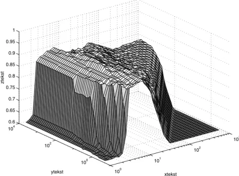
be remarked that the refining of the grid is not always necessary as the 10-fold (CV10) cross-validation performance typically has a flat maximum, as can be seen from figure 2.
In combination with the iterative algorithm of Section 5, one solves the linear systems
(17) and (18) for the first grid point starting from initial valuex0=0. For the nextγvalue in
the grid, the solutionsηandνwere initialized accordingly. When changingσ, we initialized
νandηwith the corresponding solutions related to the previousσvalue. Depending on the
distance between the points in the grid, the average reduction of the number of iteration
steps amounts to 10%–50% with respect to starting fromx0=0 for all (σ, γ) combinations.
For the polynomial kernel functions the hyperparametersγandcwere tuned by a similar
procedure, while the regularization parameter γ of the linear kernel was selected from a
refined setbased upon the cross-validation performance. For multiclass problems, the
100 101 102 103 100 102 104 0.6 0.65 0.7 0.75 0.8 0.85 0.9 0.95 1 xtekst ytekst ztekst
Figure 2. Cross-validation (CV10) classification accuracy on theiondataset as a function of the regularization parameterγ and kernel parameterσfor an LS-SVM with RBF kernel. The function of this dataset is rather flat near the maximum. The CV10 accuracy is more sensitive to the kernel or bandwidth parameterσselection (Rao, 1983) than to the choice of the regularization parameter for this dataset.
7. Benchmark results
In this section, we report on the application of LS-SVMs on 20 benchmark datasets (Blake & Merz, 1998), of which a brief description will be included in Section 7.1. The performance of the LS-SVM classifier is compared with a selection of reference techniques discussed in Section 7.2. In Sections 7.3 and 7.4 the randomized test set results are discussed. The sparse approximation procedure is illustrated in Section 7.5.
7.1. Description of the datasets
Most datasets have been obtained from the UCI benchmark repository (Blake & Merz,
1998) athttp://kdd.ics.uci.edu/. The US postal service dataset was retrieved from
the Kernel Machines website athttp://www.kernel-machines.org/. These datasets
have been referred to numerous times in the literature, which makes them very suitable for benchmarking purposes. As a preprocessing step, all records containing unknown values are removed from consideration. The following binary datasets were retrieved from Blake
and Merz (1998): the Statlog Australian credit (acr), the Bupa liver disorders (bld), the
Statlog German credit (gcr), the Statlog heart disease (hea), the Johns Hopkins university
Table 1. Characteristics of the binary classification UCI datasets.
acr bld gcr hea ion pid snr ttt wbc adu
NCV 460 230 666 180 234 512 138 638 455 33000 Ntest 230 115 334 90 117 256 70 320 228 12222 N 690 345 1000 270 351 768 208 958 683 45222 nnum 6 6 7 7 33 8 60 0 9 6 ncat 8 0 13 6 0 0 0 9 0 8 n 14 6 20 13 33 8 60 9 9 14
NCVstands for the number of data points used in the cross-validation based tuning procedure,
Ntestfor the number of observations in the test set andNfor the total dataset size. The number of
numerical and categorical attributes is denoted bynnumandncatrespectively,nis the total number
of attributes.
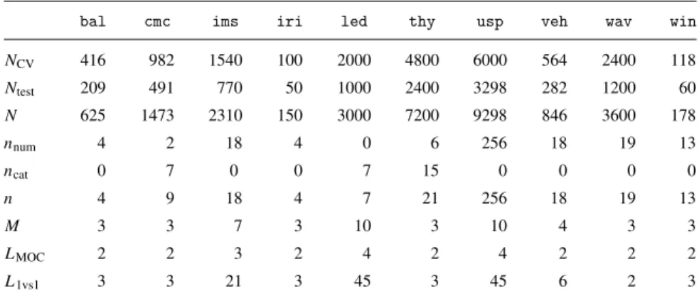
Table 2. Characteristics of the multiclass datasets.
bal cmc ims iri led thy usp veh wav win
NCV 416 982 1540 100 2000 4800 6000 564 2400 118 Ntest 209 491 770 50 1000 2400 3298 282 1200 60 N 625 1473 2310 150 3000 7200 9298 846 3600 178 nnum 4 2 18 4 0 6 256 18 19 13 ncat 0 7 0 0 7 15 0 0 0 0 n 4 9 18 4 7 21 256 18 19 13 M 3 3 7 3 10 3 10 4 3 3 LMOC 2 2 3 2 4 2 4 2 2 2 L1vs1 3 3 21 3 45 3 45 6 2 3
NCVstands for the number of data points used in the cross-validation based tuning procedure,Ntest
for the number of data in the test set andNfor the total amount of data. The number of numerical and categorical attributes is denoted bynnumandncatrespectively,nis the total number of attributes. The
Mrow denotes the number of classes for each dataset, encoded byLMOCandL1vs1bits for MOC and
1vs1 output coding, respectively.
(ttt), the Wisconsin breast cancer (wbc) and the adult (adu) dataset. The main
character-istics of these datasets are summarized in Table 1. The following multiclass datasets were
used: the balance scale (bal), the contraceptive method choice (cmc), the image
segmenta-tion (ims), the iris (iri), the LED display (led), the thyroid disease (thy), the US postal
service (usp), the Statlog vehicle silhouette (veh), the waveform (wav) and the wine
recog-nition (win) dataset. The main characteristics of the multiclass datasets are summarized in
Table 2.
7.2. Description of the reference algorithms
The test set performance of the LS-SVM classifier was compared with the performance
the decision tree algorithm C4.5 (Quinlan, 1993), Holte’s one-rule classifier (oneR) (Holte, 1993); statistical algorithms like linear discriminant analysis (LDA), quadratic discriminant analysis (QDA), logistic regression (logit) (Bishop, 1995; Duda & Hart, 1973; Ripley, 1996); instance based learners (IB) (Aha & Kibler, 1991) and Naive Bayes (John & Langley, 1995). The oneR, LDA, QDA, logit, NBk and NBn require no parameter tuning. For C4.5, we used the default confidence level of 25% for pruning, which is the value that is commonly used in the machine learning literature. We also experimented with other pruning levels on some of the datasets, but found no significant performance increases. For IB we used both 1 (IB1) and 10 (IB10) nearest neighbours. We used both standard Naive Bayes with the
normal approximation (NBn) (Duda & Hart, 1973) and the kernel approximation (NBk) for
numerical attributes (John & Langley, 1995). The default classifier or majority rule (Maj. Rule) was included as a baseline in the comparison tables. All comparisons were made on the same randomizations. For another comparison study among 22 decision tree, 9 statistical and 2 neural network algorithms, we refer to (Lim, Loh, & Shih, 2000).
The comparison is performed on an out-of-sample test set consisting of 1/3 of the data. The first 2/3 of the randomized data was reserved for training and/or cross-validation. For each algorithm, we report the average test set performance and sample standard deviation on 10 randomizations in each domain (Bay, 1999; De Groot, 1986; Domingos, 1996; Lim, Loh, & Shih, 2000). The best average test set performance was underlined and denoted in bold face for each domain. Performances that are not significantly different at the 5% level
from the top performance with respect to a one-tailed pairedt-test are tabulated in bold
face. Statistically significant underperformances at the 1% level are emphasized. Perfor-mances significantly different at the 5% level but not a the 1% level are reported in nor-mal script. Since the observations on the randomizations are not independent (Dietterich,
1998), we remark that this standardt-test is used only as a (common) heuristic to
indi-cate statistical difference between average accuracies on the ten randomizations. Ranks are assigned to each algorithm starting from 1 for the best average performance and ending with 18 and 28 for the algorithm with worst performance, for the binary and multiclass domains, respectively. Averaging over all domains, the Average Accuracy (AA) and Av-erage Rank (AR) are reported for each algorithm (Lim, Loh, & Shih, 2000). A Wilcoxon signed rank test of equality of medians is used on both AA and AR to check whether the performance of an algorithm is significantly different from the algorithm with the highest
accuracy. A Probability of a Sign Test (PST) is also reported comparing each algorithm
to the algorithm with best accuracy. The results of these significance tests on the average domain performances are denoted in the same way as the performances on each individual domain.
7.3. Performance of the binary LS-SVM classifier
In this subsection, we present and discuss the results obtained by applying the empirical setup, outlined in Section 6, on the 10 UCI binary benchmark datasets described above. All experiments were carried out on Sun Ultra5 Workstations and on Pentium II and III PCs. For the kernel types, we used RBF kernels, linear (Lin) and polynomial (Pol) kernels (with
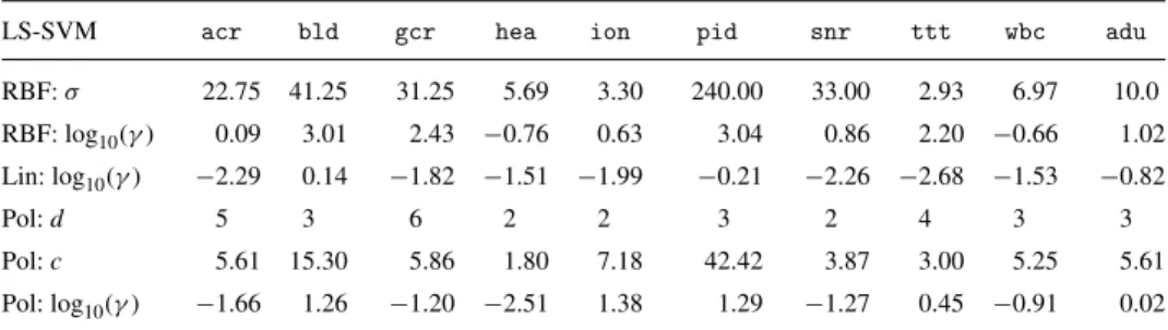
Table 3. Optimized hyperparameter values of the LS-SVMs with RBF, linear and polynomial kernels for the binary classification datasets.
LS-SVM acr bld gcr hea ion pid snr ttt wbc adu
RBF:σ 22.75 41.25 31.25 5.69 3.30 240.00 33.00 2.93 6.97 10.0 RBF: log10(γ) 0.09 3.01 2.43 −0.76 0.63 3.04 0.86 2.20 −0.66 1.02 Lin: log10(γ) −2.29 0.14 −1.82 −1.51 −1.99 −0.21 −2.26 −2.68 −1.53 −0.82 Pol:d 5 3 6 2 2 3 2 4 3 3 Pol:c 5.61 15.30 5.86 1.80 7.18 42.42 3.87 3.00 5.25 5.61 Pol: log10(γ) −1.66 1.26 −1.20 −2.51 1.38 1.29 −1.27 0.45 −0.91 0.02
Kernel Fisher Discriminant Analysis (LS-SVMF) targets{−N/N−,+N/N+}are reported.
All givenninputs are normalized to zero mean and unit variance (Bishop, 1995).
The regularization parameterγand the kernel parametersσandcof the binary LS-SVM
classifier with linear, RBF and polynomial kernel were selected from the 10-fold cross-validation procedure discussed in Section 6. The optimal values for these parameters are reported in Table 3. The flat maximum of the CV10 classification accuracy is illustrated in
figure 2 for theiondataset. This pattern was commonly encountered among all evaluated
datasets. The corresponding training, validation and test set performances are reported in Tables 5–7, respectively. The best validation and test set performances are underlined and denoted in bold face. These experimental results indicate that the RBF kernel yields the best validation and test set performance, while also polynomial kernels yield good performances. Note that we also conducted the analyses using non-scaled polynomial kernels, i.e., with
c = 1. For this scaling parameter LS-SVMs with polynomial kernels of degreesd = 2
andd =10 yielded on all domains average test set performances of 84.3% and 65.9%,
respectively. Comparing this performance with the average test set performance of 85.6%
and 85.5% (Table 7) obtained when using scaling, this clearly motivates the use of
band-width or kernel parameters. This is especially important for polynomial kernels with degree
d ≥5.
The regularization parameter C and kernel parameter σ of the SVM classifiers with
linear and RBF kernels were selected in a similar way as for the LS-SVM classifier using the 10-fold cross-validation procedure. The optimal hyperparameters of the SVM classifiers were reported in Table 4. The corresponding average test set performances are reported in Table 8.
Table 4. Optimized hyperparameter values of the SVM with RBF and linear kernel for the binary classification datasets.
SVM acr bld gcr hea ion pid snr ttt wbc adu
RBF:σ 12.43 9.0 55.0 7.15 3.30 15.50 5.09 9.00 19.5 8.00 RBF: log10(C) 2.09 1.64 3.68 −0.51 0.51 0.04 1.70 −0.41 1.86 0.70
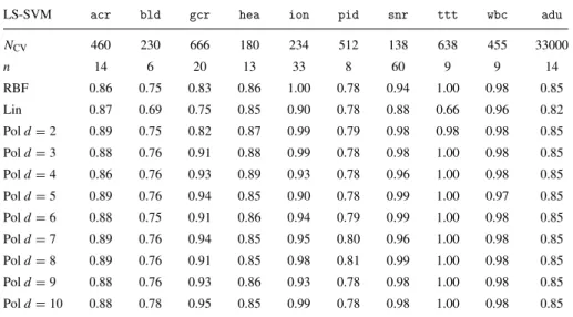
Table 5. Training setperformance of LS-SVMs on 10 binary domains.
LS-SVM acr bld gcr hea ion pid snr ttt wbc adu
NCV 460 230 666 180 234 512 138 638 455 33000 n 14 6 20 13 33 8 60 9 9 14 RBF 0.86 0.75 0.83 0.86 1.00 0.78 0.94 1.00 0.98 0.85 Lin 0.87 0.69 0.75 0.85 0.90 0.78 0.88 0.66 0.96 0.82 Pold=2 0.89 0.75 0.82 0.87 0.99 0.79 0.98 0.98 0.98 0.85 Pold=3 0.88 0.76 0.91 0.88 0.99 0.78 0.98 1.00 0.98 0.85 Pold=4 0.86 0.76 0.93 0.89 0.93 0.78 0.96 1.00 0.98 0.85 Pold=5 0.89 0.76 0.94 0.85 0.90 0.78 0.99 1.00 0.97 0.85 Pold=6 0.88 0.75 0.91 0.86 0.94 0.79 0.99 1.00 0.98 0.85 Pold=7 0.89 0.76 0.94 0.85 0.95 0.80 0.96 1.00 0.98 0.85 Pold=8 0.89 0.76 0.91 0.85 0.98 0.81 0.99 1.00 0.98 0.85 Pold=9 0.88 0.76 0.93 0.86 0.93 0.78 0.98 1.00 0.98 0.85 Pold=10 0.88 0.78 0.95 0.85 0.99 0.78 0.98 1.00 0.98 0.85
Table 6. Validation set performance of LS-SVMs on 10 binary domains, the best performances on each domain are underlined and denoted in bold face.
LS-SVM acr bld gcr hea ion pid snr ttt wbc adu
NCV 460 230 666 180 234 512 138 638 455 33000 n 14 6 20 13 33 8 60 9 9 14 RBF 0.86 0.72 0.76 0.83 0.96 0.78 0.77 0.99 0.97 0.85 Lin 0.86 0.67 0.74 0.83 0.87 0.78 0.78 0.66 0.96 0.82 Pold=2 0.86 0.72 0.76 0.83 0.91 0.78 0.82 0.98 0.97 0.84 Pold=3 0.86 0.73 0.76 0.83 0.91 0.78 0.82 0.99 0.97 0.84 Pold=4 0.86 0.72 0.77 0.83 0.78 0.78 0.81 1.00 0.97 0.84 Pold=5 0.87 0.72 0.76 0.83 0.78 0.78 0.81 1.00 0.97 0.84 Pold=6 0.86 0.73 0.77 0.83 0.78 0.78 0.81 1.00 0.97 0.84 Pold=7 0.86 0.72 0.77 0.83 0.78 0.78 0.81 1.00 0.97 0.84 Pold=8 0.86 0.73 0.76 0.83 0.78 0.78 0.81 1.00 0.97 0.84 Pold=9 0.86 0.73 0.77 0.83 0.78 0.78 0.81 0.99 0.97 0.84 Pold=10 0.86 0.71 0.77 0.83 0.91 0.78 0.81 1.00 0.97 0.84
The optimal regularization and kernel parameters were then used to assess the test set
performance of the LS-SVM and LS-SVMFclassifier on 10 randomizations: for each
ran-domization the first 2/3 of the data were used for training, while the remaining 1/3 was put aside for testing. In the same way, the test set performances of the reference algorithms were assessed. The same randomizations were used to tabulate the performances of the reference algorithms. Both sample mean and sample standard deviation of the performance
Table 7. Test setperformance of LS-SVMs on 10 binary domains, the best performances on each domain are underlined and denoted in bold face.
LS-SVM acr bld gcr hea ion pid snr ttt wbc adu
Ntest 230 115 334 90 117 256 70 320 228 12222 n 14 6 20 13 33 8 60 9 9 14 RBF 0.90 0.71 0.77 0.87 0.97 0.77 0.76 0.99 0.96 0.84 Lin 0.90 0.72 0.77 0.86 0.88 0.77 0.74 0.67 0.96 0.82 Pold=2 0.89 0.71 0.76 0.84 0.93 0.78 0.86 0.99 0.96 0.84 Pold=3 0.90 0.71 0.77 0.84 0.93 0.77 0.83 0.99 0.96 0.85 Pold=4 0.89 0.70 0.76 0.86 0.91 0.78 0.83 1.00 0.96 0.84 Pold=5 0.90 0.72 0.75 0.87 0.88 0.76 0.83 1.00 0.96 0.84 Pold=6 0.89 0.71 0.76 0.88 0.91 0.77 0.84 1.00 0.96 0.85 Pold=7 0.89 0.70 0.75 0.87 0.91 0.77 0.79 1.00 0.96 0.85 Pold=8 0.88 0.70 0.76 0.86 0.91 0.76 0.83 1.00 0.96 0.85 Pold=9 0.88 0.70 0.76 0.86 0.90 0.77 0.80 0.99 0.96 0.84 Pold=10 0.89 0.71 0.75 0.88 0.94 0.78 0.80 1.00 0.96 0.84
on the different domains are denoted in Table 8 using the bold, normal and emphasized script to enhance the visual interpretation as explained above. Averaging over all domains, the mean performance and rank and the probability of different medians with respect to the best algorithm are tabulated in the last 3 columns of Table 8.
The LS-SVM classifier with Radial Basis Function kernel (RBF LS-SVM) achieves the best average test set performance on 3 of the 10 benchmark domains, while its accuracy is not significantly worse than the best algorithm in 3 other domains. LS-SVM classifiers with polynomial and linear kernel yield the best performance on two and one datasets,
respec-tively. Also RBF SVM, IB1, NBkand C4.5 achieve the best performance on one dataset each.
Comparison of the accuracy achieved by the nonlinear polynomial and RBF kernel with the accuracy of the linear kernel illustrates that most domains are only weakly nonlinear.
The LS-SVM formulation with binary targets{−1,+1}yields a better performance than
the LS-SVMF regression formulation related to regularized kernel Fisher’s discriminant
analysis with targets{−N/N−,+N/N+}, although not all tests report a significant
differ-ence. Noticing that the LS-SVM with linear kernel and without regularization (γ → ∞)
corresponds to the LDA classifier, we also remark that a comparison of both accuracies indicates that the use of regularization slightly improves the generalization behaviour.
Considering the Average Accuracy (AA) and Average Ranking (AR) over all domains (Bay, 1999; De Groot, 1986; Domingos, 1996), the RBF SVM gets the best average accuracy and the RBF LS-SVM yields the best average rank. There is no significant difference between the performance of both classifiers. The average performance of Pol LS-SVM
and Pol LS-SVMF is not significantly different with respect to the best algorithms. The
performances of many other advanced SVM algorithms are in line with the above results (Bradley & Mangasarian, 1998; Mika et al., 1999; Sch¨olkopf, Burges, & Smola, 1998). The significance tests on the average performances of the other classifiers do not always yield
T able 8 . Comparison of the 10 times randomized test set performance of LS-SVM and LS-SVM F (linear , polynomial and Radial Basis Function k ernel) with the performance of LD A, QD A, Logit, C4.5, oneR, IB1, IB10, NB k ,N Bn and the Majority Rule classifier on 10 binary domains. acr bld gcr hea ion pid snr ttt wbc adu AA AR PST Ntest 230 115 334 90 117 256 70 320 228 12222 n 14 6 2 0 1 33 386 0 9 91 4 RBF LS-SVM 87.0 (2.1) 70.2 (4.1) 76.3 (1.4) 84.7 (4.8) 96.0 (2.1) 76.8 (1.7) 73.1 (4.2) 99.0 (0.3) 96.4 (1.0) 84.7 (0.3) 84.4 3.5 0.727 RBF LS-SVM F 86.4 (1.9) 65.1 (2.9) 70.8 (2.4) 83.2 (5.0) 93.4 (2.7) 72.9 (2.0) 73.6 (4.6) 97.9 (0.7) 96.8 (0.7) 77.6 (1.3) 81.8 8.8 0.109 Lin LS-SVM 86.8 (2.2) 65.6 (3.2) 75.4 (2.3) 84.9 (4.5) 87.9 (2.0) 76.8 (1.8) 72.6 (3.7) 66.8 (3.9) 95.8 (1.0) 81.8 (0.3) 79.4 7.7 0.109 Lin LS-SVM F 86.5 (2.1) 61.8 (3.3) 68.6 (2.3) 82.8 (4.4) 85.0 (3.5) 73.1 (1.7) 73.3 (3.4) 57.6 (1.9) 96.9 (0.7) 71.3 (0.3) 75.7 12.1 0.109 Pol LS-SVM 86.5 (2.2) 70.4 (3.7) 76.3 (1.4) 83.7 (3.9) 91.0 (2.5) 77.0 (1.8) 76.9 (4.7) 99.5 (0.5) 96.4 (0.9) 84.6 (0.3) 84.2 4.1 0.727 Pol LS-SVM F 86.6 (2.2) 65.3 (2.9) 70.3 (2.3) 82.4 (4.6) 91.7 (2.6) 73.0 (1.8) 77.3 (2.6) 98.1 (0.8) 96.9 (0.7) 77.9 (0.2) 82.0 8.2 0.344 RBF SVM 86.3 (1.8) 70.4 (3.2) 75.9 (1.4) 84.7 (4.8) 95.4 (1.7) 77.3 (2.2) 75.0 (6.6) 98.6 (0.5) 96.4 (1.0) 84.4 (0.3) 84.4 4.0 1.000 Lin SVM 86.7 (2.4) 67.7 (2.6) 75.4 (1.7) 83.2 (4.2) 87.1 (3.4) 77.0 (2.4) 74.1 (4.2) 66.2 (3.6) 96.3 (1.0) 83.9 (0.2) 79.8 7.5 0.021 LD A 85.9 (2.2) 65.4 (3.2) 75.9 (2.0) 83.9 (4.3) 87.1 (2.3) 76.7 (2.0) 67.9 (4.9) 68.0 (3.0) 95.6 (1.1) 82.2 (0.3) 78.9 9.6 0.004 QD A 80.1 (1.9) 62.2 (3.6) 72.5 (1.4) 78.4 (4.0) 90.6 (2.2) 74.2 (3.3) 53.6 (7.4) 75.1 (4.0) 94.5 (0.6) 80.7 (0.3) 76.2 12.6 0.002 Logit 86.8 (2.4) 66.3 (3.1) 76.3 (2.1) 82.9 (4.0) 86.2 (3.5) 77.2 (1.8) 68.4 (5.2) 68.3 (2.9) 96.1 (1.0) 83.7 (0.2) 79.2 7.8 0.109 C4.5 85.5 (2.1) 63.1 (3.8) 71.4 (2.0) 78.0 (4.2) 90.6 (2.2) 73.5 (3.0) 72.1 (2.5) 84.2 (1.6) 94.7 (1.0) 85.6 (0.3) 79.9 10.2 0.021 oneR 85.4 (2.1) 56.3 (4.4) 66.0 (3.0) 71.7 (3.6) 83.6 (4.8) 71.3 (2.7) 62.6 (5.5) 70.7 (1.5) 91.8 (1.4) 80.4 (0.3) 74.0 15.5 0.002 IB1 81.1 (1.9) 61.3 (6.2) 69.3 (2.6) 74.3 (4.2) 87.2 (2.8) 69.6 (2.4) 77.7 (4.4) 82.3 (3.3) 95.3 (1.1) 78.9 (0.2) 77.7 12.5 0.021 IB10 86.4 (1.3) 60.5 (4.4) 72.6 (1.7) 80.0 (4.3) 85.9 (2.5) 73.6 (2.4) 69.4 (4.3) 94.8 (2.0) 96.4 (1.2) 82.7 (0.3) 80.2 10.4 0.039 NB k 81.4 (1.9) 63.7 (4.5) 74.7 (2.1) 83.9 (4.5) 92.1 (2.5) 75.5 (1.7) 71.6 (3.5) 71.7 (3.1) 97.1 (0.9) 84.8 (0.2) 79.7 7.3 0.109 NB n 76.9 (1.7) 56.0 (6.9) 74.6 (2.8) 83.8 (4.5) 82.8 (3.8) 75.1 (2.1) 66.6 (3.2) 71.7 (3.1) 95.5 (0.5) 82.7 (0.2) 76.6 12.3 0.002 Maj. rule 56.2 (2.0) 56.5 (3.1) 69.7 (2.3) 56.3 (3.8) 64.4 (2.9) 66.8 (2.1) 54.4 (4.7) 66.2 (3.6) 66.2 (2.4) 75.3 (0.3) 63.2 17.1 0.002 The A v erage Accurac y (AA), A v erage Rank (AR) and Probability of equal medians using the Sign T est (PST ) tak en o v er all domains are reported in the last three columns. Best performances are underlined and denoted in bold face, performances not significantly dif ferent at the 5% le v el are denoted in bold face, performances significantly dif ferent at the 1% le v el are emphasized.
the same results. Generally speaking, the performance of Lin LS-SVM, Lin SVM, Logit and
NBkis not significantly different at the 1% level. Also the performances of LS-SVMs with
Fisher’s discriminant targets (LS-SVMF) are not signifantly different at the 1%. Generally
speaking, the results of Table 8 allow to conclude that the SVM and LS-SVM formulations achieve very good test set performances compared to the other reference algorithms.
7.4. Performance of the multiclass LS-SVM classifier
We report the performance of multiclass LS-SVMs on 10 multiclass categorization prob-lems. Each multiclass problem is decomposed into a set of binary classification problems using minimum output coding (MOC) and one-versus-one (1vs1) output coding. The same kernel types as for the binary domain were considered: RBF kernels, linear (Lin) and
poly-nomial (Pol) kernels with degreesd =2, . . . ,10. Both the performance of LS-SVM and
LS-SVMFclassifiers are reported. The MOC and 1vs1 output coding were also applied to
SVM classifiers with linear and RBF kernels. As for the binary domains, we normalized the inputs to zero mean and unit variance (Bishop, 1995).
The experimental setup of the previous section is used: each binary classifier of the multiclass LS-SVM is designed on the first 2/3 of the data using 10-fold cross-validation, while the remaining 1/3 are put aside for testing. The selected regularization and kernel
parameters3were then fixed and 10 randomizations were conducted on each domain. The
average test set accuracies of the different LS-SVM and LS-SVMFclassifiers, with RBF,
Lin and Pol kernel (d =2, . . . ,10) and using MOC and 1vs1 output coding, are reported in
Table 9. The test set accuracies of the reference algorithms on the same randomizations are
also reported, where we remark that for theuspdataset the memory requirements for logit
were too high. Instead, we tabulated the performance of LDA instead of logit for this single case. The same statistical tests as in Section 7.3 were used to compare the performance of the different classifiers.
The use of QDA yields the best average test set accuracy on two domains, while LS-SVMs
with 1vs1 coding using a RBF and Lin kernel and LS-SVMFwith Lin kernel each yield the
best performance on one domain. SVMs with RBF kernel with MOC and 1vs1 coding yield the best performance on one domain each. Also C4.5, logit and IB1 each achieve one time the best performance. The use of 1vs1 coding generally results into a better classification accuracy. Averaging over all 10 multiclass domains, the LS-SVM classifier with RBF kernel and 1vs1 output coding achieves the best average accuracy (AA) and average ranking, while its performance is only on three domains significantly worse at 1% than the best algorithm. This performance is not significantly different from the SVM with RBF kernel and 1vs1 output coding. Summarizing the different significant tests, RBF SVM (MOC), Pol
LS-SVM (MOC), Lin LS-LS-SVM (1vs1), Lin LS-LS-SVMF(1vs1), Pol LS-SVM (1vs1), RBF SVM
(MOC), RBF SVM (1vs1), Lin SVM (1vs1), LDA, QDA, Logit, C4.5, IB1 and IB10 perform
not significantly different at the 5% level. While NBkperformed well on the binary domains,
its average accuracy on the multiclass domains is never comparable at the 5% level for all three tests. The overall results of Table 9 illustrate that the SVM and LS-SVM classifier with RBF kernel using 1vs1 output coding consistently yield very good test set accuracies on the multiclass domains.
T able 9 . Comparison of the 10 times randomized test set performance of LS-SVM and LS-SVM F (linear , polynomial and Radial Basis Function k ernel) with the performance of LD A, QD A, Logit, C4.5, oneR, IB1, IB10, NB k ,N Bn and the Majority Rule classifier on 10 multiclass domains. LS-SVM bal cmc ims iri led thy usp veh wav win AA AR PST Ntest 209 491 770 50 1000 2400 3298 282 1200 60 n 49 1 8 4 7 21 256 18 19 13 RBF LS-SVM (MOC) 92.7 (1.0) 54.1 (1.8) 95.5 (0.6) 96.6 (2.8) 70.8 (1.4) 96.6 (0.4) 95.3 (0.5) 81.9 (2.6) 99.8 (0.2) 98.7 (1.3) 88.2 7.1 0.344 RBF LS-SVM F (MOC) 86.8 (2.4) 43.5 (2.6) 69.6 (3.2) 98.4 (2.1) 36.1 (2.4) 22.0 (4.7) 86.5 (1.0) 66.5 (6.1) 99.5 (0.2) 93.2 (3.4) 70.2 17.8 0.109 Lin LS-SVM (MOC) 90.4 (0.8) 46.9 (3.0) 72.1 (1.2) 89.6 (5.6) 52.1 (2.2) 93.2 (0.6) 76.5 (0.6) 69.4 (2.3) 90.4 (1.1) 97.3 (2.0) 77.8 17.8 0.002 Lin LS-SVM F (MOC) 86.6 (1.7) 42.7 (2.0) 69.8 (1.2) 77.0 (3.8) 35.1 (2.6) 54.1 (1.3) 58.2 (0.9) 69.1 (2.0) 55.7 (1.3) 85.5 (5.1) 63.4 22.4 0.002 Pol LS-SVM (MOC) 94.0 (0.8) 53.5 (2.3) 87.2 (2.6) 96.4 (3.7) 70.9 (1.5) 94.7 (0.2) 95.0 (0.8) 81.8 (1.2) 99.6 (0.3) 97.8 (1.9) 87.1 9.8 0.109 Pol LS-SVM F (MOC) 93.2 (1.9) 47.4 (1.6) 86.2 (3.2) 96.0 (3.7) 67.7 (0.8) 69.9 (2.8) 87.2 (0.9) 81.9 (1.3) 96.1 (0.7) 92.2 (3.2) 81.8 15.7 0.002 RBF LS-SVM (1vs1) 94.2 (2.2) 55.7 (2.2) 96.5 (0.5) 97.6 (2.3) 74.1 (1.3) 96.8 (0.3) 94.8 (2.5) 83.6 (1.3) 99.3 (0.4) 98.2 (1.8) 89.1 5.9 1.000 RBF LS-SVM F (1vs1) 71.4 (15.5) 42.7 (3.7) 46.2 (6.5) 79.8 (10.3) 58.9 (8.5) 92.6 (0.2) 30.7 (2.4) 24.9 (2.5) 97.3 (1.7) 67.3 (14.6) 61.2 22.3 0.002 Lin LS-SVM (1vs1) 87.8 (2.2) 50.8 (2.4) 93.4 (1.0) 98.4 (1.8) 74.5 (1.0) 93.2 (0.3) 95.4 (0.3) 79.8 (2.1) 97.6 (0.9) 98.3 (2.5) 86.9 9.7 0.754 Lin LS-SVM F (1vs1) 87.7 (1.8) 49.6 (1.8) 93.4 (0.9) 98.6 (1.3) 74.5 (1.0) 74.9 (0.8) 95.3 (0.3) 79.8 (2.2) 98.2 (0.6) 97.7 (1.8) 85.0 11.1 0.344 Pol LS-SVM (1vs1) 95.4 (1.0) 53.2 (2.2) 95.2 (0.6) 96.8 (2.3) 72.8 (2.6) 88.8 (14.6) 96.0 (2.1) 82.8 (1.8) 99.0 (0.4) 99.0 (1.4) 87.9 8.9 0.344 Pol LS-SVM F (1vs1) 56.5 (16.7) 41.8 (1.8) 30.1 (3.8) 71.4 (12.4) 32.6 (10.9) 92.6 (0.7) 95.8 (1.7) 20.3 (6.7) 77.5 (4.9) 82.3 (12.2) 60.1 21.9 0.021 RBF SVM (MOC) 99.2 (0.5) 51.0 (1.4) 94.9 (0.9) 96.6 (3.4) 69.9 (1.0) 96.6 (0.2) 95.5 (0.4) 77.6 (1.7) 99.7 (0.1) 97.8 (2.1) 87.9 8.6 0.344 Lin SVM (MOC) 98.3 (1.2) 45.8 (1.6) 74.1 (1.4) 95.0 (10.5) 50.9 (3.2) 92.5 (0.3) 81.9 (0.3) 70.3 (2.5) 99.2 (0.2) 97.3 (2.6) 80.5 16.1 0.021 RBF SVM (1vs1) 98.3 (1.2) 54.7 (2.4) 96.0 (0.4) 97.0 (3.0) 64.6 (5.6) 98.3 (0.3) 97.2 (0.2) 83.8 (1.6) 99.6 (0.2) 96.8 (5.7) 88.6 6.5 1.000 Lin SVM (1vs1) 91.0 (2.3) 50.8 (1.6) 95.2 (0.7) 98.0 (1.9) 74.4 (1.2) 97.1 (0.3) 95.1 (0.3) 78.1 (2.4) 99.6 (0.2) 98.3 (3.1) 87.8 7.3 0.754 LD A 86.9 (2.1) 51.8 (2.2) 91.2 (1.1) 98.6 (1.0) 73.7 (0.8) 93.7 (0.3) 91.5 (0.5) 77.4 (2.7) 94.6 (1.2) 98.7 (1.5) 85.8 11.0 0.109 QD A 90.5 (1.1) 50.6 (2.1) 81.8 (9.6) 98.2 (1.8) 73.6 (1.1) 93.4 (0.3) 74.7 (0.7) 84.8 (1.5) 60.9 (9.5) 99.2 (1.2) 80.8 11.8 0.344 Logit 88.5 (2.0) 51.6 (2.4) 95.4 (0.6) 97.0 (3.9) 73.9 (1.0) 95.8 (0.5) 91.5 (0.5) 78.3 (2.3) 99.9 (0.1) 95.0 (3.2) 86.7 9.8 0.021 C4.5 66.0 (3.6) 50.9 (1.7) 96.1 (0.7) 96.0 (3.1) 73.6 (1.3) 99.7 (0.1) 88.7 (0.3) 71.1 (2.6) 99.8 (0.1) 87.0 (5.0) 82.9 11.8 0.109 oneR 59.5 (3.1) 43.2 (3.5) 62.9 (2.4) 95.2 (2.5) 17.8 (0.8) 96.3 (0.5) 32.9 (1.1) 52.9 (1.9) 67.4 (1.1) 76.2 (4.6) 60.4 21.6 0.002 IB1 81.5 (2.7) 43.3 (1.1) 96.8 (0.6) 95.6 (3.6) 74.0 (1.3) 92.2 (0.4) 97.0 (0.2) 70.1 (2.9) 99.7 (0.1) 95.2 (2.0) 84.5 12.9 0.344 IB10 83.6 (2.3) 44.3 (2.4) 94.3 (0.7) 97.2 (1.9) 74.2 (1.3) 93.7 (0.3) 96.1 (0.3) 67.1 (2.1) 99.4 (0.1) 96.2 (1.9) 84.6 12.4 0.344 NB k 89.9 (2.0) 51.2 (2.3) 84.9 (1.4) 97.0 (2.5) 74.0 (1.2) 96.4 (0.2) 79.3 (0.9) 60.0 (2.3) 99.5 (0.1) 97.7 (1.6) 83.0 12.2 0.021 NB n 89.9 (2.0) 48.9 (1.8) 80.1 (1.0) 97.2 (2.7) 74.0 (1.2) 95.5 (0.4) 78.2 (0.6) 44.9 (2.8) 99.5 (0.1) 97.5 (1.8) 80.6 13.6 0.021 Maj. rule 48.7 (2.3) 43.2 (1.8) 15.5 (0.6) 38.6 (2.8) 11.4 (0.0) 92.5 (0.3) 16.8 (0.4) 27.7 (1.5) 34.2 (0.8) 39.7 (2.8) 36.8 24.8 0.002 The A v erage Accurac y (AA), A v erage Rank (AR) and Probability of equal medians using the Sign T est (P ST ) tak en o v er all domains are reported in the last three columns. The notation of T able 8 is used to report the results of the significance tests.
7.5. LS-SVM sparse approximation procedure
The sparseness property of SVMs is lost in LS-SVMs by the use of a 2-norm. While the generalization capacity is still controlled by the regularization term, the use of a smaller number of support vectors may be interesting to reduce the computational cost of evaluating
the classifier for new inputsx. We illustrate the sparse approximation procedure (Suykens &
Vandewalle, 1999b; 1999c; Suykens et al., 2002) of Section 4 on 10 datasets for LS-SVMs with RBF kernel.
The amount of pruning was estimated by means of 10-fold cross-validation. In each pruning step, 5% of the support values of each training set were pruned and the classification accuracy was assessed on the corresponding validation set. The hyperparameters were re-estimated on a small local grid when the cross-validation performance decreased. This local optimization of the hyperparameters is carried out in order to prune more support values at the expense of an increased computational cost. Then, the next pruning step was performed. This pruning procedure was stopped when the cross-validation performance decreased
significantly using a paired one-tailedt-test compared with the initial performance (when
no pruning was applied) or with the previous performance. Both 1% and 5% Significance Levels were used and are denoted by SL1% and SL5%, respectively. Given the number of
Pruning Steps #PSSL5%and #PSSL1%and the optimal hyperparameters for each step from
the cross-validation procedure, the pruning is now performed in the same way on the whole
cross-validation set starting from NCVsupport values down to NSL5%and NSL1%support
values and the accuracies of the LS-SVM, LS-SVMSL5%and LS-SVMSL1%on the test set
are reported. An example of the evolution of the cross-validation and test set performance
for thewbcdataset as a function of the number of pruning steps is depicted in figure 3. For
multiclass domains, 1vs1 coding was used and the sparse approximation procedure was applied to each binary classifier.
This pruning procedure was applied on the first 5 binary and first 5 multiclass prob-lems studied above, using LS-SVMs with RBF kernels and with 1vs1 output coding for
the multiclass problems. The resulting randomized test set accuracies of the LS-SVMSL5%
and LS-SVMSL1%are tabulated in Table 10, corresponding to pruning till SL5% and SL1%
significance levels, respectively. The results of applying no pruning at all (LS-SVM) are
repeated on the first row. A one-tailed pairedt-test is used to highlight statistical
differ-ences from the best algorithm on each domain in the same way as in Tables 8 and 9. In most cases, the SL5% and SL1% stop criterion yield no significant difference in the number of pruning steps and the resulting number of support values, while the mance generally decreases not significantly. Experimentally we observe that the perfor-mance on a validation set stays constant or increases slightly when pruning. After a cer-tain time, the performance starts decreasing rather fast as the pruning continues. This ex-plains the small difference in the number of pruned training examples when using the 5% and 1% stopping criterion. Averaging over all datasets, we find that the sparse ap-proximation procedure does not yield significantly different results at the 1% level. From a comparison with Tables 8 and 9, we conclude that this procedure allows a firm re-duction of the number of training examples, while still a good test set performance is obtained.