Instance sampling in credit scoring: An empirical study of sample size and balancing

(1)

Contents lists available atSciVerse ScienceDirect

International Journal of Forecasting

journal homepage:www.elsevier.com/locate/ijforecast

Instance sampling in credit scoring: An empirical study of sample size

and balancing

Sven F. Crone

1

,

Steven Finlay

∗ Lancaster University, United Kingdom

a r t i c l e i n f o Keywords: Credit scoring Data pre-processing Sample size Under-sampling Over-sampling Balancing

a b s t r a c t

To date, best practice in sampling credit applicants has been established based largely on expert opinion, which generally recommends that small samples of 1500 instances each of both goods and bads are sufficient, and that the heavily biased datasets observed should be balanced by undersampling the majority class. Consequently, the topics of sample sizes and sample balance have not been subject to either formal study in credit scoring, or empirical evaluations across different data conditions and algorithms of varying efficiency. This paper describes an empirical study of instance sampling in predicting consumer repayment behaviour, evaluating the relative accuracies of logistic regression, discriminant analysis, decision trees and neural networks on two datasets across 20 samples of increasing size and 29 rebalanced sample distributions created by gradually under- and over-sampling the goods and bads respectively. The paper makes a practical contribution to model building on credit scoring datasets, and provides evidence that using samples larger than those recommended in credit scoring practice provides a significant increase in accuracy across algorithms.

1. Introduction

The vast majority of consumer lending decisions, whether to grant credit to individuals or not, are made us-ing automated credit scorus-ing systems based on individuals’ credit scores. Credit scores provide an estimate of whether an individual is a ‘‘good’’ or ‘‘bad’’ credit risk (i.e. a binary classification), and are generated using predictive models of the repayment behaviours of previous credit applicants whose repayment performances have been observed over a period of time (Thomas, Edelman, & Crook, 2002). A large credit granting organization will have millions of customer records and recruit hundreds of thousands of new cus-tomers each year. Although this provides a rich source of

∗_{Correspondence to: Management Science, Lancaster University,} Management School, Lancaster, United Kingdom. Tel.: +44 1772 798673.

E-mail addresses:[email protected](S.F. Crone), [email protected](S. Finlay).

1 Tel.: +44 1524 5 92991; fax: +44 1524 844885.

data upon which credit scoring models can be constructed, the size of the customer databases means that they of-ten prove ineffective or inefficient (given the cost, resource and time constraints) for developing predictive models us-ing the complete customer database. As a consequence, the standard practice has been for credit scoring models to be constructed using samples of the available data. This places particular importance on the methods applied for constructing the samples which will later be used to build accurate and reliable credit scoring models.

Despite its apparent relevance, past research in credit scoring has not systematically evaluated the effect of in-stance sampling. Rather than follow insights based upon empirical experiments of sample size and balance, cer-tain recommendations expressed by industry experts have received wide acceptance within the credit scoring com-munity and practitioner literature, driven by the under-standing that customer databases in credit scoring show a high level of homogeneity between different lenders and across geographic regions. In particular, the advice of

Lewis(1992) andSiddiqi(2006) is generally taken, based

(2)

on their considerable experience of scorecard devel-opment. With regard to a suitable sampling strategy, both propose random undersampling in order to address class imbalances, and suggest that a sample containing 1500–2000 instances of each class (including any valida-tion sample) should be sufficient for building robust high quality models. Given the size of empirical databases, this is equivalent to omitting large numbers of instances of both the majority class of ‘goods’ and the minority class of ‘bads’. Although this omits potentially valuable segments of the total customer sample from the model building pro-cess, these recommendations have not been substantially challenged, either in practice or in academic research, the latter of which has focussed instead on comparing the ac-curacies of different predictive algorithms on even smaller and more unbalanced datasets. As a consequence, issues of sample size and balancing have been neglected within the credit scoring community as a topic of study.

Issues of constructing samples for credit scoring have only received attention in the area of reject inference, which has emphasised sampling issues relating to the selection bias introduced as a result of previous decision making in credit scoring, and the application of techniques to adjust for this bias (Banasik & Crook, 2007; Kim & Sohn, 2007;Verstraeten & Van den Poel, 2005). However, this research does not consider the more practical issues of efficient and effective sample sizes and (im-)balances. Therefore, beyond a common sense agreement that larger sample sizes are beneficial and smaller ones are more efficient, the issue of determining an efficient sample size and sample distribution (balancing) to enhance the predictive accuracy of different algorithms on the available data has not been considered. (Similarly, limited attention has been paid in credit scoring to other data preprocessing issues, such as feature selection — seeLiu & Schumann, 2005; Somol, Baesens, Pudil, & Vanthienen, 2005 — or transformation — see e.g. Piramuthu, 2006 — which are deemed important but are beyond this discussion.) Considering that data and their preparation are considered to be the most crucial and time-consuming aspect of any scorecard development (Anderson, 2007), this omission is surprising and indicates a significant gap in the research.

In contrast to credit scoring, issues of sample imbal-ances have received a substantial amount of attention in data mining, leading to the development of novel tech-niques, e.g., using instance creation to balance sampling (Chawla, Bowyer, Hall, & Kegelmeyer, 2002), frameworks for modelling rare data (Weiss, 2004), and best prac-tices for oversampling through instance resampling (for an overview seeChawla, Japkowicz, & Kolcz, 2004), which have not been explored in the area of credit scoring. Since proven alternatives to instance sampling exist, they war-rant a discussion and empirical assessment for their appli-cation to credit scoring.

In this paper, two aspects of the sampling strategy are explored in regard to their empirical impact on model per-formance for datasets of credit scoring structure: sample size and sample balance. Section2reviews the prior re-search, in both best practice and empirical studies, and identifies a gap in the research on instance sampling. Both the sample size and the balance are discussed, with re-flections as to whether the sample size remains an issue

for scorecard developers today, given the computational resources available, and investigating how random over-sampling and underover-sampling may aid in predictive mod-elling. An empirical study is then described in Section3, examining the relationship between the sample strategy and the predictive performance for two industry-supplied data sets, both larger (and more representative) than those published in research to date: one an application scoring data set, the other a behavioural scoring data set. A wide variety of sampling strategies are explored, in the form of 20 data subsets of gradually increasing size, together with 29 samples of class imbalances by gradually over- and under-sampling the number of goods and bads in each sub-set respectively. Having looked at both sample sizes and balancing in isolation, the final part of the paper consid-ers the interaction between sample sizes and balancing and looks at the way in which predictive performance co-varies with each of these dimensions. All of the results from the sampling strategy are assessed across four compet-ing classification techniques, which are well established and are known to have practical applications within the financial services industry: Logistic Regression (LR), Lin-ear Discriminant Analysis (LDA), Classification and Regres-sion Trees (CART) and artificial Neural Networks (NN). The empirical evaluation seems particularly relevant in light of the differences between the statistical efficiencies of the estimators with regard to the sample size and distribu-tion, e.g. the comparatively robust Logistic Regression ver-sus Discriminant Analysis (see, e.g.Hand & Henley, 1993). Consequently, we anticipate different sensitivity (or rather robustness) levels across different classifiers, which may explain their relative performances, beyond practical rec-ommendations to increase sample sizes and/or balance distributions across algorithms in practice.

2. Instance selection in credit scoring

2.1. Best practices and empirical studies in sampling The application of algorithms for credit scoring requires data in a mathematically feasible format, which is achieved through data preprocessing (DPP) in the form of data re-duction, with the aim of decreasing the size of the datasets by means of instance selection and/or feature selection, and data projection, thus altering the representation of data, e.g. by the categorisation of continuous variables. In order to assess prior research on instance selection for credit scoring, best practice recommendations (from prac-titioners) are reviewed in contrast to the experimental se-tups employed in prior empirical academic studies.

In credit scoring practice, the various recommenda-tions as to sample size concur with the original advice of

Lewis(1992) and Siddiqi(2006), that 1500 instances of each class (goods, bads and indeterminates) should be suf-ficient to build robust, high quality models (see e.g.

An-derson,2007;Mays,2001;McNab & Wynn, 2003, amongst others). This includes data for validation, although this re-quires fewer cases, perhaps a minimum of 300 of each (Mays, 2001). Anderson (2007) justifies the validity of these sample size recommendations empirically, as both Anderson and Siddiqi have worked in practice for many

(3)

years and the recommendations appear to be sufficiently large to reduce the effects of multicolinearity and overfit-ting when working with correlated variables. However, he points out that no logic has been provided for the choice of these numbers, which were determined in the 1960s when the collection of data was more costly, and that their use has continued ever since without further eval-uation or challenge (Anderson, 2007), although in prac-tice larger samples are sometimes taken where available (Hand & Henley, 1997;Thomas et al.,2002).

The considered validity of these recommendations is founded upon the understanding that customer databases in credit scoring are homogeneous across lenders and re-gions. Indeed, the majority of lenders ask similar questions on application forms (Finlay,2006;Thomas et al.,2002), and use standardized industry data sources such as those supplied by credit reference agencies. Although credit ref-erence data vary from agency to agency, the general types of consumer data supplied by credit reference agencies worldwide are broadly the same, containing a mixture of credit history, public information and geo-demographic data (Jentzsch,2007;Miller,2003). Consequently, datasets are homogeneous regarding the features which have pre-dictive power, i.e. these customer characteristics. (Note that we do not consider special cases of sparse and im-balanced credit datasets, such as low default portfolios, to which these characteristics and later findings do not ap-ply.) However, as credit scoring activities are carried out by a range of organisations, from banks and building soci-eties to retailers, other dataset attributes will differ (Hand & Henley, 1997). The sizes of datasets, although generally considered ‘large’, will vary from ubiquitous data on retail credit to fewer customers for wholesale credit (Anderson, 2007). Similarly, the sample distributions of datasets, al-though generally biased towards the goods and with rela-tively few bads, will vary to reflect the different risks of the lending decision. Empirical class imbalances range from around 2

:

1 of goods to bads for some sub-prime port-folios to over 100

:

1 for high quality mortgage portfolios. It is not clear how recommendations hold across heteroge-neous variations of dataset properties.

Table 1summarizes the algorithms and data conditions of sample sizes and sample balances from a structured lit-erature review of academic publications which have em-ployed multiple comparisons of credit scoring algorithms and methodologies (thus eliminating a range of papers evaluating a single algorithm, or minor tuned variants).

Table 1documents the emphasis on applying and tun-ing multiple classification algorithms for a given dataset sample, in contrast to evaluating the effect of instance se-lection in credit scoring. The review yields two conclu-sions:

(a) Academic studies in credit scoring have ignored possible DPP parameters relating to sample size and sample distribution. If sample size and/or sample imbalances were to have a significant impact on predictive accuracy of some algorithms, the results across various different studies in credit scoring might be impaired.

(b) The datasets used in academic studies do not reflect the empirical recommendations from credit scoring practice: the relative accuracy of algorithms is assessed across much smaller datasets than 1500 instances in each class, and datasets are left imbalanced (of the original sample distribution). This questions the representativeness of prior academic findings for practice, and their comparability across datasets with substantially different data conditions. Furthermore, this echoes similar important omissions in other areas of corporate data mining, such as direct marketing (Crone, Lessmann, & Stahlbock, 2006), and warrants a systematic empirical evaluation across data conditions. As a further observation, most studies seem to be pre-occupied with the predictive accuracy, but fail to reflect other objectives such as interpretability and resource ef-ficiency (in both time and costs), which also determine the empirical adequacy of different algorithms in practice. Be-yond accuracy, the interpretability of models — and there-fore whether the model is in line with the intuition of the staff — is often of even greater importance; while speed (the speed of classification itself and the speed with which a score-card can be revised) and robustness are also rele-vant (see e.g.Hand & Henley, 1997). Various computational intelligence methods, such as NN and SVM, have been re-ported to outperform standard regression approaches by a small margin (Baesens et al., 2003), in terms of accu-racy, but are not used widely due to their perceived com-plexity, increased resources and reduced interpretability. As a consequence, logistic regression remains the most popular method applied by practitioners working within the financial services industry (Crook, Edelman, & Thomas, 2007;Thomas, Oliver, & Hand, 2005), offering a suitable balance of accuracy, efficiency and interpretability. Dis-criminant analysis (DA) and Classification and Regression Trees (CART) are also popular, due to the relative ease with which models can be developed, their limited opera-tional requirements, and particularly their interpretability (Finlay, 2008). As the DPP choices in sample size and bal-ance may impact not only the accuracy, but also the inter-pretability and efficiency of the algorithms, the discussion of experimental results will need to reflect possible trade-offs between objectives while assessing the relative per-formance of algorithms across different data conditions. Furthermore, as the algorithms exhibit different levels of statistical efficiency, we expect changes in the relative per-formance of some of the algorithms (i.e., DA in contrast to the robust LR, see e.g.Hand & Henley, 1993).

2.2. Sample size

Instance sampling is a common approach in statistics and data mining, and is used both for a preliminary inves-tigation of the data and to facilitate efficient and effective model building on large datasets, by selecting a represen-tative subset of a population for model construction (Tan, Steinbach, & Kumar, 2006). The data sample should ex-hibit approximately the same properties of interest (i.e., the mean of the population, or the repayment behaviour in credit scoring) as the original set of data, such that the

(4)

Table 1

Methods and samples used in empirical studies on credit scoring.

Study Methods1 _{Dataset and samples}

LDA LR NN KNN CART Other Data sets Good cases2 _{Bad cases}2, 3 _{Goods: bads Indep. vars.} Boyle, Crook, Hamilton, and Thomas

(1992)

X X hyb.LDA 1 662 139 4.8:1 7 to 24

Henley(1995) X X X X PP, PR 1 6851 8203 0.8:1 16

Desai, Conway, Crook, and Overstreet(1997)4

X X X GA 1 714 293 2.4:1 18

Arminger, Enache, and Bonne(1997) X X X 1 1390 1294 1.1:1 21

West(2000) X X X X X KD 2 360 270 1.3:1 24

276 345 0.8:1 14

Baesens et al.(2003) X X X X X QDA 8 466 200 2.3:1 20

BC 455 205 2.2:1 14 SVM 1056 264 4.0:1 19 LP 2376 264 9.0:1 19 1388 694 2.0:1 33 3555 1438 2.5:1 33 4680 1560 3.0:1 16 6240 1560 4.0:1 16

Ong, Huang, and Gwo-Hshiung(2005) X X X GP, RS 2 246 306 0.8:1 26

560 240 2.3:1 31

1_BC₌_{Bayes Classifiers, CART}₌_{Classification and Regression Trees, GA}₌_{Genetic Algorithm, GP}₌_{Genetic Programming, KD}₌_{Kernel Density,}

KNN=K-Nearest Neighbour, LDA=Linear Discriminant Analysis, LP=Linear Programming, LR=Logistic Regression, NN=Neural Networks, QDA=Quadratic Discriminant Analysis, PP=Projection Pursuit, PR=Poisson Regression, RS=Rough sets, SVM=Support Vector Machines.

2_{In some studies, the number of goods/bads used for estimating the model parameters is not given. In these cases, the number of goods/bads has been}

inferred from information provided about the total sample size, the proportion of goods and bads and the development/validation methodology applied.

3_{This is the number of variables used for parameter estimation after pre-processing.}

4_{Three data sets from different credit unions were used, and the models were estimated using both the individual data sets and a combined data set.}

The figures quoted are for the combined data set.

discriminatory power of a model built on a sample is com-parable to that of one built on the full dataset. Larger sam-ple sizes increase the probability that a samsam-ple will be representative of the population, and therefore ensure similar predictive accuracy, but also eliminate many of the advantages of sampling, such as reduced computation times and data acquisition costs. In smaller samples, the patterns contained in the data may be missed or erroneous patterns may be detected, thus enhancing efficiency at the cost of limiting accuracy. Therefore, determining an effi-cient and effective sample size requires a methodical ap-proach, given the properties of the datasets, in order to balance the trade-off between accuracy and resource effi-ciency, assuming that the interpretability of the models is not impacted.

Although empirical sample sizes in credit scoring will vary by market size, market share and credit application, most data sets are large. In the UK, Barclaycard has over 11 million credit card customers, and recruited more than 1 million new card customers in 2008 (Barclay’s, 2008). In the US, several organizations, such as Capital One, Bank of America and Citigroup, have consumer credit portfolios containing tens of millions of customer accounts (Evans & Schmalensee, 2005). Samples are conventionally built using a stratified random sample (without replacement) on the target variable, either drawing an equal number of goods and bads in proportion to the size of that group in the population (unbalanced), or using equal numbers of instances of each class (balanced). Consequently, the limiting factor for sample sizes is often the number of bads, with few organizations having more than a few thousand, or at most tens of thousands, of bad cases (Anderson, 2007). From a theoretical perspective, at first sight, the issue of larger sample sizes might appear to have been resolved in

recent years due to the increased computational resources provided by a modern PC. Credit scoring models using popular approaches such as LR, LDA and CART can be developed within a few hours using large samples of observations. Since using the entire available dataset, rather than sampling from it, has now become a feasible course of action for most consumer credit portfolios, it is valid to ask: is the issue of the sample size still relevant for scorecard development? In practical situations, the sample size does still remain an important issue for a range of reasons. First, there are often costs associated with acquiring data from a credit reference agency, resulting in a trade-off between the increase in accuracy obtained from using larger samples and the marginal cost of acquiring additional data. Also, a model developer may rebuild a model many times, possibly even dozens of times, to ensure that the model meets the business requirements that are often imposed on such models, or to evaluate the effect of different DPPs or different meta-parameters of algorithms, in order to enhance performance. This means that even small reductions in the time required to estimate the parameters of a single model on a sample may result in large and significant reductions in the project time/cost when many iterations of model development occur. In contrast, when sub-population models are considered, larger samples may be required. It may be relatively easy to construct a sub-population model and confirm that it generates unbiased estimates, but if the sample upon which it has been developed is too small, then a locally constructed sub-population model may not perform as effectively as a model developed on a larger, more general population, despite the statistical efficiency of the estimator. In the case of population drift, where applicant populations and distributions evolve over time due to

(5)

changes in the competitive and economic environment (Hand & Henley, 1997), not all records of past applicants are representative of current/future behaviour, and hence sampling is required. This has been particularly apparent in the recent credit crunch, where new models have needed to be constructed for the novel economic circumstances (Hand,2009a,b), thus limiting the ability to use all data and raising the question as to what the minimum (or near optimal) sample size for a renewed scorecard development would be. Consequently, larger samples are not always desirable. Rather, the trade-off between accuracy and computational costs must be considered in order to derive resource efficient and effective decisions with respect to the sample size.

Furthermore, some algorithms are expected to perform better on larger samples of data, whilst others are more efficient at utilizing a given training sample when esti-mating parameters. For example, NN and SVM generally outperform LR when applied to credit scoring problems (Crook et al., 2007), but when the sample sizes are small, LR may generate better performing models due to the smaller number of parameters requiring estimation. In contrast, when datasets get very large, NN are considered to bene-fit from the additional data, while the performance of SVM would suffer. This implies that the sample size should be considered alongside other features when deciding upon the algorithm, and may explain previous inconsistent re-sults on the relative accuracy of the same methods across credit scoring studies for different sample sizes.

2.3. Sample distribution (balancing)

For real-world credit scoring datasets, the target variable is predominantly imbalanced, with the majority of instances composed of normal examples (‘‘goods’’) and only a small percentage of abnormal or interesting examples (‘‘bads’’). A dataset is said to be unbalanced if the number of instances in each category of the target variable is not (approximately) equal, which is the case across most applications in both credit scoring and data mining.

The importance of reflecting the imbalance between the majority and minority classes in modelling is not primarily an algorithmic one, but is often derived from the underlying decision context and the costs associated with it. In many applications, the costs of type I and type II errors is dramatically asymmetrical, making an invalid prediction of the minority class more costly than an accurate prediction of the majority class. However, traditional classification algorithms — driven by the objective of minimising some loss of error function across two different segments of a population — typically have a bias towards the majority class, which provides more error signals. Therefore, the underlying problem requires either the development of distribution insensitive algorithms or an artificial rebalancing of the datasets through sampling.

Problems of data driven model building with imbal-anced classes are not uncommon in other domains of corporate data mining, such as response rates in direct marketing, and are ubiquitous in classification tasks across a range of disciplines (see e.g. the special issue byChawla et al., 2004). In instance sampling, random over- and

undersampling methodologies have received particular at-tention (Weiss & Provost, 2003). In undersampling, in-stances of the minority and majority classes are selected randomly in order to achieve a balanced stratified sample with equal class distributions, often using all instances of the minority class and only a sub-set of the majority class, or undersampling both classes for even smaller subsets with equal class sizes. Alternatively, in oversampling, the cases of the under-represented class are replicated a num-ber of times, so that the class distributions are more equal. Note that inconsistencies in this terminology are frequent, and also arise in credit scoring (e.g.Anderson, 2007, mis-takenly refers to oversampling, but essentially describes simple undersampling by removing instances of the ma-jority class).

Under- and over-sampling generally lead to models with a enhanced discriminatory power, but both random oversampling and random undersampling methods have their shortcomings: random undersampling can discard potentially important cases from the majority class of the sample (the goods), thus impairing an algorithm’s ability to learn the decision boundary; while random oversam-pling duplicates records and can lead to the overfitting of similar instances. (Note that under- and over-sampling are only conducted on the training data used for model development, while the original class distributions are retained for the out-of-sample test data.) Therefore, un-dersampling tends to overestimate the probability of cases belonging to the minority class, while oversampling tends to underestimate the likelihood of observations belong-ing to the minority class (Weiss, 2004). As both over-and under-sampling can potentially reduce the accuracy in generalisation for unseen data, a number of studies have compared variants of over- and under-sampling, and have presented (often conflicting) viewpoints on the accuracy gains derived from oversampling versus undersampling (Chawla,2003;Drummond & Holte, 2003;Maloof,2003;

Prati, Batista, & Monard, 2004), indicating that the results are not universal and depend on the dataset properties and the application domain. However, as datasets in credit scoring have similar properties across lenders, the findings on over- vs. under-sampling are expected to be more rep-resentative across databases.

Reflecting on best practices and empirical studies (see Section2.1), credit scoring practices actively recommend and exclusively employ undersampling, while academic studies have predominantly used the natural distribu-tion of the imbalanced classes (see Table 1). Both have ignored the various oversampling approaches developed in data mining, and the evidence of the impaired accu-racy caused by removing potentially valuable instances from the sample through undersampling. More sophisti-cated approaches to under- and over-sampling have been developed, e.g. selectively undersampling unimportant instances (Laurikkala, 2002) or creating synthetic exam-ples in oversampling (Chawla et al., 2002), in addition to other alternatives such as cost sensitive learning. How-ever, in the absence of an evaluation of even simple approaches to imbalanced instance sampling in credit scoring, these are omitted for the benefit of a sys-tematic evaluation of different intensities of over- and

(6)

under-sampling. It should be noted that we later assess under- and over-sampling on empirical datasets which are subject to an inherent sample selection bias towards applicants who were previously considered creditworthy. Possible remedies of reject inference are ignored in this analysis. However, as instance sampling techniques of over- and under-sampling merely provide different error signals from the information contained within the original sample, and do not augment the sample for missing parts of the population, we suspect the effect of instance sam-pling techniques to be complementary to choices of reject inference.

Moreover, the error signals derived from different num-bers of goods and bads may shift the decision surface in feature space for those methods estimating decision boundaries using fundamentally different approaches to classifier design, depending on their statistical efficiency. LR estimates the probability (P) that an applicant with a particular vectorxof characteristic levels is good directly, withP

(

g

|•

)

, while the LDA estimates and the probabil-ity densprobabil-ity function of the good-risk applicants will be denoted by p

(

•|

g

)

and p

(

•|

b

)

for bads respectively, and P

(

g

|•

)

is then derived (seeHand & Henley, 1993, for a more elaborate discussion). Algorithms such as NN offer addi-tional degrees of freedom in model building, beyond those of LR, which may yield different levels of statistical effi-ciency. For example, a NN may consider the prediction of goods directly by employing a single output node to esti-mateP

(

g

|•

)

(essentially modelling a conventional LR with multiple latent variables, depending on the number of hid-den nodes), by using two indepenhid-dent output nodes to as-sessp

(

•|

g

)

andp

(

•|

b

)

to deriveP

(

g

|•

)

, as in LDA, or by using combinations by linking multiple output nodes us-ing the softmax function, which pose undefined statisti-cal properties and efficiency. Should these meta-parameter choices impact the estimator efficiency, as well as increas-ing the number of parameters to be estimated through la-tent variables, different practical recommendations for an effective dataset size and balance may be the result.

The effect of balancing on estimators of different statis-tical efficiency should be assessed separately to the effect of sample sizes, or the joint effect of the sample distri-bution and sample size. This assessment will be problem-atic for strong undersampling, since, by creating very small samples, the parameters may deviate from the population value somewhat, due to the inherent variance in smaller samples, despite ensuring random sampling throughout all of the experiments. To reflect this, our experiments will also include small sample sizes, not to compare classifiers of different statistical efficiency across these small sam-ples, but rather to replicate the inconsistent findings of many academic studies. It is anticipated that small sample sizes should result in inconsistencies in relative classifier accuracy levels, caused predominantly by experimental biases introduced through the arbitrarily chosen small sample size, but not in the classifiers’ capabilities (i.e., non-linearity etc.) or the sample distribution of the data. Such findings would confirm the findings of previous studies, and hence add to the reliability of our findings, and place our assessment of the sample size and balance in the con-text of the existing research.

Furthermore, it should be noted that over- and under-sampling will impact not only the predictive accuracy, depending on the statistical efficiency, but also the resource efficiency in model construction and application. Balancing has an impact on the total sample size by omitting or replicating good and/or bad instances, thereby decreasing or increasing the total number of instances in the dataset, which impacts the time taken for model parameterisation (although this seems less important than improving the accuracy, as the time taken to apply an estimated model will remain unchanged).

3. Experimental design

3.1. Datasets

Two datasets, both of which are substantially larger than those used in empirical studies to date (seeTable 1), were used in the study, taken from the two prominent sub-areas of credit and behavioural scoring.

The first dataset (datasetA) was supplied by Experian UK, and contained details of credit applications made between April and June 2002. Performance information was attached 12 months after the application date. The Experian-provided delinquency status was used to generate a 1

/

0 target variable for modelling purposes (good

=

1, bad

=

0). Accounts which were up-to-date, or no more than one month in arrears, and which had not been seriously delinquent within the last 6 months (three months or more in arrears) were classified as good. Those that were currently three or more months in arrears, or had been three months in arrears at any time within the last 6 months, were classified as bad. This is consistent with the good/bad definitions commonly reported in the literature as being applied by practitioners, based on bads being three or more cycles delinquent and goods as up-to-date or no more than one cycle delinquent (Hand & Henley, 1997;Lewis,1992;McNab & Wynn, 2003). After the removal of outliers and indeterminates, the sample contained 88,789 observations, of which 75,528 were classified as good and 13,261 as bad. 39 independent variables were available in setA. The independent variables included common application form characteristics such as age, residential status and income, as well as UK credit reference data, including the number, value and time since the most recent CCJ/bankruptcy, current and historical account performance, recent credit searches, and Electoral Roll and MOSAIC postcode level classifiers.

The second dataset, datasetB, was a behavioural scoring data set from a mail order catalogue retailer providing revolving credit. Performance data were attached as at 12 months after the sample date. The good/bad definition provided by the data provider was similar to that for set A. Goods were defined as being no more than one month in arrears, bads as being three or more months in arrears at the outcome point. After exclusions such as newly opened accounts (less than 3 months old), dormant accounts (maximum balance on the account within the last 3 months

=

£0), accounts already in a serious delinquency status (currently 2

+

payments in arrears), and those classified as indeterminate (neither good nor bad), the

(7)

sample contained 120,508 goods and 18,098 bads. Dataset Bcontained 55 independent variables, examples of which were current and historic statement balances, current and historic arrears status, payment to balance ratios, and so on.

3.2. Sample size

The first part of the study looked at the effects of in-creasing the sample size on the predictive performance. For the purpose of the study, and to ensure valid and re-liable estimates of the experimental results despite some small sample sizes, we employedk-fold random cross-validation across all experiments, essentially replicating each random samplek

=

50 times (i.e., resampling). For each of the two datasets, a set of subsamples of different size were constructed using the following procedure:

Step 1. The population ofNobservations, comprising Ggoods andBbads (N

=

G

+

B) was segmented into ksections of equal size, withppercentiles within each fold. Stratified random sampling was applied, with the goods and bads sampled independently to ensure that the class priors in each section and percentile matched that of the distribution in the population.

Step 2. Ak-fold development/validation methodology was applied to constructkmodels for each cumulative ppercentage of the population. The number of obser-vations used to construct each model,N_p, was there-fore equal toN

∗ [

p

∗

(

k

−

1

)/

k

]

/

100.Npg andNpbare the number of goods and bads used to construct each model, such thatNp

=

Npg

+

Npb. For each model, all N

/

kobservations in the validation section were used to evaluate the model performance.

Values ofpranging from 5% to 100% were considered in increments of 5%, in order to evaluate any consistent and gradual effects of the sample size variation on accuracy, leading to 20 different sample sizes. For a relationship between the sample size and accuracy, we would expect consistent, statistically significant results of increasing accuracy (i.e., a monotonically increasing trend of improving performance for the results to be considered reliable) beyond the recommended ‘‘best practice’’ sample size of 1500–2000 bads. The number of percentiles was chosen under the constraint of the available observations and the number of variables, so that all of the variables would still contain significant numbers of observations and allow stable parameter estimates when the sample sizes were small (a minimum of 250 bads and 500 goods for p

=

5). To comply with what is reported to be standard practice within the credit scoring community, balanced data sets were used, with the goods being randomly under-sampled (excluded) from each section for model development, so that the number of goods and bads was the same.

3.3. Balancing sample distributions

The second part of the study considered balancing. In data mining in general, studies to date have been con-ducted using undersampling on the original distribution

of the population, or oversampling on algorithms of vary-ing statistical efficiency. However, this does not allow for inference on the possible systematic and continuous ef-fects of decreasing the number of instances from the ma-jority class (undersampling) or increasing the number of the minority class (oversampling) during stratified sam-pling. Therefore, for this part of the experiment multiple random samples of gradually increasing class imbalances were created from the full data set (i.e. p

=

100), with a different balancing applied to each sample. In to-tal, 29 different balancings were applied. For descriptive purposes we refer to each balancing using the notationB_x. The 29 different balancings were chosen on the basis of expert opinion, taking into account computation require-ments and the need to obtain a reasonable number of ex-amples across the range.

To create each undersampled data set, observations were randomly excluded from the majority class (the goods) to achieve the desired number of cases. B12

represents the original class imbalanced sample. Samples B1–B11 were randomly under-sampled to an increasing

degree of class imbalance, withB3representing standard

undersampling, with the goods sampled down to equal the number of bads, and B2 undersampling the goods

beyond the number of bads (i.e., fewer goods than bads). B13–B22were randomly oversampled with increasing class

imbalances, with sampleB22representing standard

over-sampling, with the bads re-sampled so that the number of goods and bads was equal. ForB23–B29, the oversampling

was extended further, so that the samples contained more bads than goods.

This creates a continuous, gradually increasing imbal-ance from extreme undersampling to extreme oversam-pling, spanning most of the sampling balances employed in data mining, while allowing us to observe possible ef-fects from a smooth transition of accuracy due to sample imbalances.

To create the oversampled data sets, each member of the minority class (the bads) was sampled INT

(

Npv

/

Npb

)

times, whereNpvis the desired number of bads in the sam-ple (thus, for standard over-sampling, where the number of bads is equal to the number of goods,Npv

=

Npg). An addi-tional (Npv

−

INT

(

Npv

/

Npb

)

) bads were then randomly sam-pled without replacement, so that the sample contained the desired number of observations

(

Npv

)

. Thek-fold devel-opment/validation methodology described in Section3.1

was adopted, with the observations assigned to the same 50 sections. Note that no balancing was ever applied to the test section; i.e., the class priors within the test section were always the same as those in the unbalanced parent population from which it was sampled.

The third and final part of the analysis considered the sample size and balancing in combination. The balancing experiments described previously were repeated for values of pranging from 5% to 100% in increments of 5. In theory, this allows a 3-D surface to be plotted to show how the sample size, balancing and performance co-vary, and makes it possible to consider trade-offs between the sample size and balancing. It is noted that part 3 represents a superset of experiments, containing all of those described in parts 1 and 2, as well as many others. We have taken this approach, building up the results in stages, to increase the readability of the paper.

(8)

3.4. Methods, data pre-processing and variable selection The methods were chosen to represent those estab-lished in credit scoring, including LR, LDA and CART, as well as NN, a frequently evaluated contender which has shown an enhanced accuracy in fraud detection and other back-end decision processes (where limited explicability is re-quired, see e.g.Hand, 2005), but which has failed to prove its worth in credit scoring so far. As the evaluation of dif-ferent modelling techniques is not of primary interest in this study, recently developed methods such as SVM are not assessed.

The experiments were repeated for LR, LDA, CART and NN. For the CART and NN models, the development sample was further split 80

/

20 for training/validation using stratified random sampling. For CART, a large tree was initially grown using the training sample, then pruning was applied using the 20% validation sample, as advocated by Quinlan (1992). Binary splits were employed, based on maximum entropy. For NN, a MLP architecture with a single hidden layer was adopted. Preliminary experiments were performed in order to determine the number of hidden units for the hidden layer using the smallest available sample size (i.e.p

=

5), to ensure that overfitting did not result for small sample sizes.T

−

1 exploratory models were created using 2

,

3

, . . . ,

Thidden units, where T was equal to the number of units in the input layer. The number of hidden units was then chosen, based on the model performance on the 20% test sample. Given the size and dimensions of the datasets involved and the number of experiments performed, we employed a quasi-newton algorithm with a maximum of 100 training iterations, in order to allow the experiments to be completed in a realistic period of time.

The most widely adopted approach to pre-processing credit scoring data sets is to categorize the data using dummy variables (Hand & Henley, 1997), which generally provides a good linear approximation of the non-linear features of the data (Fox, 2000). Continuous variables such as income and age are binned into a number of discrete categories and a dummy variable is used to represent each bin.Hand(2005) suggests that between 3 and 6 dummies should be sufficient in most cases, although a greater number of dummies may be defined if a sufficient volume of data is available. For datasetsAand B, the independent variables were a mixture of categorical, continuous and semi-continuous variables, which were coded as dummy variables for LDA, LR, NN. All of the dummy variables in each dataset contained in excess of 500 good and 250 bad cases, and more than 1000 observations in total (for p

=

100). For CART, preliminary experiments showed that the performance based on dummy variables was extremely poor, and a better performance resulted from creating an ordinal range using the dummy variable definitions. This ordinal categorization was therefore used for CART. We note that the results of this particular data preprocessing strategy may be biased against some of the nonlinear algorithms (Crone et al., 2006), but it was chosen due to its prevalence in credit scoring practice and academic studies. To allow the experiments to be replicated, additional details on the data preprocessing and method parameterisation can be obtained from the authors upon request.

3.5. Performance evaluation

For measuring the model accuracy, a precise estimate of the likelihood of class membership may serve as a valid objective of parameterisation; however, it is of secondary importance to a model’s ability to accurately discriminate between the two classes of interest (Thomas, Banasik, & Crook, 2001). As a consequence, measures of group sep-aration, such as the area under the ROC curve (AUC), the GINI coefficient and the KS statistic, are used widely for as-sessing model performance, especially in situations where the use of the model is uncertain prior to model devel-opment, or where multiple cut-offs are applied at differ-ent points in the score distribution. Performance measures must also be insensitive to the class distribution, given the data properties of credit scoring (i.e., simple classi-fication rates may not be applied). A popular metric in data mining, the AUC, provides a single valued perfor-mance measure

[

0

;

1

]

which assesses the tradeoff between hits and false alarms, where random variables score 0.5. To employ a performance measure which is more com-mon in the practice of the retail banking sector, we assess the model performance using the related GINI coeffi-cient, calculated using the brown formula (Trapezium rule): GINI

=

1

−

n

−

i=2 [G

(

i

)

+

G

(

i

−

1

)

] [B

(

i

)

−

B

(

i

−

1

)

]

,

where S is the ranked model score and G

(

S

)

and B

(

S

)

are the cumulative proportion of good and bad cases, re-spectively, scoring

≤

Sfor allS. GINI is an equivalent trans-formation of the AUC (Hand & Henley, 1997), measuring twice the area between the ROC-curve and the diagonal (with AUC

=

(Gini

+

1)/2), to assess the true positive rate against the false positive rate. GINI measures the discrimi-natory power over all possible choices of threshold (rather than the accuracy of probability estimates of class mem-bership), which satisfies the unconditional problem of an unknown threshold or cost ratio in which GINI is consid-ered advantageous (see, e.g., the third scenario ofHand, 2005), and which adequately reflects our empirical model-ing objective. Furthermore, it allows the results to be com-pared directly with other studies, including applications in retail banking where practitioners regularly employ GINI, which is considered to be equally important. Therefore, de-spite recent criticism (see e.g.Hand,2005,2009a,b), the limited theoretical weaknesses of GINI seem to be out-weighed by its advantages in interpretability, both by prac-titioners and across other studies.

4. Experimental results

4.1. Effect of sample size

The first stage of the analysis considers the predictive accuracy of methods constructed using different sample sizes for equally distributed classes (in the training data) using undersampling. The results of the sample size experiments are presented inTable 2.

Table 2 shows both the comparative level of accu-racy between methods and changes in the accuaccu-racy for

(9)

Table 2

Absolute GINI by sample size for datasetsAandB.

p(%) DatasetA DatasetB

# Goods/bads LDA LR CART NN # Goods/bads LDA LR CART NN

5 663 0.704** _0.702** _0.572** _0.660** ₉₀₄ _0.610** _0.604** _0.536** _0.572** 10 1 326 0.721** _0.721** _0.605** _0.692** _{1 809} _0.635** _0.633** _0.542** _0.600** 15 1 989 0.727** _0.730** _0.634** _0.701** _{2 714} _0.641** _0.640** _0.548** _0.605** 20 2 652 0.729** _0.733** _0.638** _0.707** _{3 619} _0.646** _0.645** _0.556** _0.614** 25 3 315 0.730** _0.733** _0.634** _0.711** _{4 524} _0.649** _0.648** _0.567** _0.624** 30 3 978 0.731** _0.735* _0.637** _0.717** _{5 429} _0.649** _0.649** _0.574** _0.624** 35 4 641 0.732* _0.736* _0.638** _0.722** _{6 334} _0.650** _0.650** _0.572** _0.628** 40 5 304 0.733 0.736* _0.644** _0.723** _{7 239} _0.651** _0.651** _0.572** _0.633** 45 5 967 0.733 0.737 0.648** _0.725** _{8 144} _0.652** _0.652** _0.577** _0.635** 50 6 630 0.733 0.737 0.656** _0.726** _{9 049} _0.652** _0.652** _0.581** _0.637** 55 7 293 0.733 0.737 0.658** _0.727** _{9 953} _0.652** _0.653** _0.576** _0.636** 60 7 956 0.733 0.737 0.654** _0.729** _{10 858} _0.653** _0.653** _0.577** _0.637** 65 8 619 0.733 0.737 0.659** _0.730** _{11 763} _0.653** _0.654** _0.578** _0.644** 70 9 282 0.733 0.738 0.658** _0.730** _{12 668} _0.654** _0.655** _0.578** _0.644** 75 9 945 0.733 0.738 0.656** _0.731* _{13 573} _0.654** _0.655** _0.580** _0.645** 80 10 608 0.734 0.738 0.659** _0.731* _{14 478} _0.654* _0.655** _0.583** _0.646** 85 11 271 0.734 0.738 0.663* _0.731* _{15 383} _0.655* _0.656* _0.579** _0.648** 90 11 934 0.734 0.738 0.663 0.732 16 288 0.655 0.656 0.581** _0.649** 95 12 597 0.734 0.738 0.664 0.732 17 193 0.655 0.656 0.582** _0.650 100 13 261 0.734 0.738 0.664 0.732 18 098 0.655 0.656 0.588 0.651

*_{Indicates that the performance is significantly different from}_p₌_{100% at the 95% level of significance.} **_{Indicates that the performance is significantly different from}_p₌_{100% at the 99% level of significance.}

each individual method as the sample size increases.

Table 2also shows the results from pairedt-tests for de-termining whether there is a statistically significant dif-ference in performance between p

=

100, the largest possible sample available, and models constructed using samples containing onlyp

=

x% [goods/bads] (5

≤

x

≤

100). Observing the monotonically increasing signifi-cance of the results, the pairedt-test is considered a valid proxy for more comprehensive non-parametric tests of re-peated measures. It therefore provides a plausible assess-ment of the asymptotic relative efficiencies of different classification algorithms, as indicated earlier, with LR and LDA already approaching this level at 5000 bads, while NN require more than double the number of instances (while still not achieving the accuracy of LR).

Table 2 documents two original findings. First, all of the methods show monotonic increases in their predictive accuracies (with minor fluctuations in accuracy for CART), which might be considered unsurprising given the common practical understanding that more data is better. However, the accuracy increases well beyond the recommended ‘‘best practice’’ sample size of 1500–2000 instances of each class. For logistic regression and LDA, around 5000 samples of ‘bads’ are required before the performance is statistically indistinguishable from that resulting from a sample size of p

=

100 for dataset A, while around 15,000 cases are required for dataset B. This results in significantly larger (balanced) datasets of 10,000 and 30,000 instances altogether, respectively, which far exceeds both the recommendations of practice and the experimental design of academic studies. Equally, CART and NN require larger samples before their accuracy asymptotically approaches a maxmimum value, but again datasets of a larger magnitude yield further performance improvements. It is important to note that these tests of significance between samples of size p

=

x and p

=

100 should only be considered as lower bounds

on the optimal sample size, because the study has been limited by the number of observations in the data set, rather than the theoretical maximum possible number of observations (i.e. N

=

∞

). Another factor is the fact that the numbers of observations within each coarse classed interval were chosen so that when the sample sizes were small (e.g.p

=

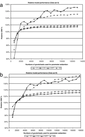
5), all of the variables would still contain a sufficient number of observations of each class to allow valid parameter estimation. In real world modelling situations, a larger number of dummy variable categories could be defined when large samples are used, which could be expected to result in an improvement in the performance of the resulting models.

The effects of an increased sample size on the algorithm performance are also illustrated in Fig. 1, which shows the relative increase in accuracy of each method, indexed relative to the results that are obtained from using the industry best practice recommendation of 1500 instances, obtained via undersampling (=100%), for both dataset A (Fig. 1(a)) and datasetB(Fig. 1(b)).

Note that Fig. 1provides the relative improvements for each of the methods in isolation, and does not compare the performances of the methods.Fig. 1shows similar patterns for models developed using datasets A andB, indicating a similar trend in performance with an increasing sample size. Increasing the sample sizes from 1500 to the maximum possible, improved the performance by 1.78% for LR, 1.40% for LDA, 5.11% for NN and 7.11% for CART on datasetA. On datasetB, the improvements were even more substantial, significantly increasing the performance by 3.14% for LDA, 3.72% for LR, 8.41% for NN and 8.48% for CART (although it should be noted that the absolute performance of CART was consistently worse than that of the other methods for both data sets, following the trend seen in Table 2). As statistically significant improvements are also feasible from simply increasing the sample size for the well explored and comparatively

(10)

a

b

Fig. 1. Relative model performance by sample size for data setsA(a) and B(b).

efficient estimator LR, well beyond its best practices, these findings provide novel and significant advancements for credit scoring practice. All increases may be considered to be substantial, considering the flat maximum effect (Lovie & Lovie, 1986) and the costs associated with increasing the scorecard accuracy by fractions of a percentage point. Furthermore, the differences due to the sample size are substantial, considering the improvements in performance attributed to algorithm choices and tuning in the literature (see, e.g.,Table 1).

The issue of an effective and efficient sample size, and of an asymptotic relative efficiency for each algorithm, is also visible in the relative performance graphs. The relative unit increase in performance of LR and LDA reduces steadily as Npbrises above 2000, plateauing at aroundNpb

=

5000 for datasetAand 12,000 for datasetB, indicating little need for larger datasets to be collected. However, for NN and CART it would appear that the performance has not plateaued byN100b, and therefore, the absolute performance might improve if larger samples were available.

The second prominent feature of Table 2 is that the relative performances of the different methods vary with the sample size, particularly for small samples. One concern which might be raised from the experimental design of the sample size is the possibility of over-fitting for small values ofNpb, when the ratio of observations to independent variables is low. If the 1

:

10 rule quoted by Harrell for logistic regression is taken as a guide (Harrell,

Lee, & Mark, 1996), then this suggests that there is a risk of over-fitting whereNpb

≤

810 (p

≤

6; i.e. the first row in Table 3 and the first data point in Fig. 1). However, the region whereNpb

≤

810 is not the area of greatest interest. Also, because of the preliminary variable selection procedure, variables have only been included in the models where there is a high degree of certainty that a relationship between the dependent and independent variables exists. It is also true that the ratio of events to variables tends to be a less important factor for large samples containing hundreds of cases of each class than for smaller samples (Steyerberg, Eijkemans, Harrell, Habbema, & Dik, 2000). Therefore, we think it unlikely that over-fitting has occurred.

We conclude that increasing the sample size beyond current best practices increases the accuracy significantly for all forecasting methods considered, despite the possible negative implications for resource efficiency in model building. Moreover, the individual methods show different sensitivities to the sample size, which allows us to infer that statistical efficiency may provide one explanation for the inconsistent results on the relative performances of different classification methods on small credit scoring datasets of varying sizes, allowing LDA, LR or possibly NN to outperform other methods, depending purely on the (un-)availability of data.

4.2. Effect of balancing

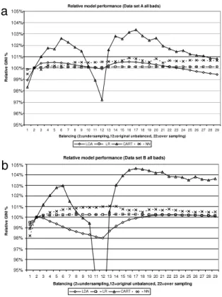
The second set of analyses reviews the effect on the predictive accuracy of balancing the distribution of the target variable.Table 3provides the results for different sample distributionsBnusing all available data (p

=

100), indicating the joint effect of changing both the sampling proportions for each of the classes and the sample sizes as a result of rebalancing.

Fig. 2provides a graphical representation of the results. In examining the results fromTable 3andFig. 2, we shall begin with the performance of logistic regression. Logistic regression is remarkably robust to balancing, yielding

>

99.7% of the maximum performance for both data sets, regardless of the balancing strategy applied. For both data sets, undersampling leads to worse performances than either the unbalanced data set

(

B12

)

or oversampling

(

B22

)

, and using the unbalanced data gives slightly worse

performances than oversampling. However, none of these differences are statistically significant. LDA displays a greater sensitivity, with its performance falling to just under 99.4% for dataset A and 98% for dataset B. For both datasets, the worst performances for LDA are when B12 is applied, and these differences are significant at

the 99% significance level. CART is by far the most sensitive technique, with a maximum performance of 95% for datasetAand 84% for datasetB. NN also shows some sensitivity to balancing, with a performance which worsens, the greater the degree of undersampling applied. Another feature displayed inFig. 2, and arguably the most interesting one, is that the maximum performance does not always occur at the traditional over-sampling point (B22). For dataset A, the optimal balancing is at

(11)

Table 3

Absolute GINI by sample distribution for datasetsAandB.

Bn DatasetA DatasetB

Goods Bads LDA LR CART NN Goods Bads LDA LR CART NN 807 13,261 0.692 0.729 0.477 0.699 1 7,034 13,261 0.726 0.737 0.653 0.728 7,857 18,098 0.650 0.653 0.582 0.639 2 13,261 13,261 0.734 0.738 0.664 0.732 18,098 18,098 0.655 0.656 0.588 0.651 3 19,485 13,261 0.737 0.739 0.671 0.731 28,339 18,098 0.654 0.657 0.595 0.652 4 25,712 13,261 0.738 0.739 0.676 0.734 38,580 18,098 0.653 0.657 0.601 0.653 5 31,939 13,261 0.738 0.739 0.675 0.734 48,821 18,098 0.651 0.658 0.605 0.654 6 38,166 13,261 0.737 0.739 0.681 0.734 59,062 18,098 0.649 0.658 0.606 0.655 7 44,393 13,261 0.737 0.739 0.679 0.735 69,303 18,098 0.647 0.658 0.597 0.656 8 50,620 13,261 0.736 0.739 0.676 0.736 79,544 18,098 0.646 0.658 0.591 0.656 9 56,847 13,261 0.735 0.739 0.674 0.736 89,785 18,098 0.645 0.658 0.588 0.657 10 63,074 13,261 0.735 0.739 0.665 0.736 100,026 18,098 0.644 0.658 0.585 0.657 11 69,301 13,261 0.734 0.739 0.657 0.736 110,267 18,098 0.643 0.658 0.552 0.657 12 75,528 13,261 0.733 0.739 0.645 0.736 120,508 18,098 0.642 0.658 0.518 0.657 13 75,528 19,488 0.736 0.739 0.675 0.737 120,508 28,339 0.646 0.658 0.592 0.657 14 75,528 25,715 0.737 0.739 0.683 0.737 120,508 38,580 0.650 0.658 0.606 0.657 15 75,528 31,942 0.738 0.739 0.681 0.737 120,508 48,821 0.652 0.658 0.612 0.656 16 75,528 38,169 0.738 0.739 0.685 0.739 120,508 59,062 0.653 0.658 0.615 0.655 17 75,528 44,396 0.738 0.739 0.686 0.738 120,508 69,303 0.654 0.658 0.616 0.655 18 75,528 50,623 0.737 0.739 0.683 0.737 120,508 79,544 0.655 0.658 0.615 0.654 19 75,528 56,850 0.737 0.739 0.680 0.736 120,508 89,785 0.656 0.658 0.614 0.655 20 75,528 63,077 0.736 0.739 0.681 0.738 120,508 100,026 0.656 0.658 0.613 0.655 21 75,528 69,304 0.735 0.739 0.677 0.736 120,508 110,267 0.656 0.658 0.614 0.655 22 75,528 75,528 0.735 0.739 0.675 0.737 120,508 120,508 0.657 0.657 0.611 0.656 23 75,528 81,755 0.734 0.739 0.674 0.737 120,508 130,749 0.657 0.657 0.611 0.655 24 75,528 87,982 0.733 0.739 0.674 0.737 120,508 140,990 0.657 0.657 0.611 0.654 25 75,528 94,209 0.733 0.739 0.672 0.737 120,508 151,231 0.656 0.657 0.609 0.654 26 75,528 100,436 0.732 0.739 0.671 0.737 120,508 161,472 0.656 0.657 0.611 0.654 27 75,528 106,663 0.731 0.739 0.671 0.737 120,508 171,713 0.656 0.657 0.609 0.654 28 75,528 112,890 0.730 0.739 0.670 0.737 120,508 181,954 0.656 0.657 0.609 0.654 29 75,528 119,117 0.730 0.739 0.669 0.737 120,508 192,195 0.656 0.657 0.610 0.654 B2=standard undersampling (goods=number of bads),B12=the original unbalanced data set, andB22=standard oversampling (bads=number of

goods).

For datasetB, the optimal balancing occurs atB14

,

B23

,

B17

andB13for LR, LDA, CART and NN respectively. We suspect

that the application of a single over- or under-sampling strategy will be sub-optimal for some sub-regions within the problem domain. For example, it is quite possible that bads are actually the majority class in some regions, and therefore, a more appropriate strategy for this region would be to oversample goods, not bads. This leads us to propose that one further area of study be the application of a regional sub-division algorithm, such as clustering, followed by the application of separate balancings to each of the resulting clusters. Alternatively, a preliminary model could be constructed, with balancing applied based on the posterior probability estimates from the preliminary model.

The results confirm the results of previous studies on related datasets, e.g. on large datasets with strong imbal-ances in direct marketing (Crone et al., 2006), supporting their validity. In analysing our results, it is apparent that changes to the sample distribution lead to different loca-tions of the decision boundary and classificaloca-tions of un-seen instances, caused by altered cumulative error signals during parameterisation (for a visualisation of shifted deci-sion boundaries, albeit on another aspect of sample selec-tion bias, see e.g.Wu & Hand, 2007). Further evidence of this can be found in the changed coefficients of LR and NN (which may be interpreted directly for a given variable), at times even changing the sign of the coefficient, which

one may be less concerned with if one is interested pri-marily in increases in predictive accuracy. However, this may have implications for the interpretation of the model, and would require a thorough evaluation in practice. Also, possible interactions with initiatives to adjust for reject in-ference should be evaluated carefully, in order to assess whether they are fully compatible.

4.3. Joint effect of sample size and balancing

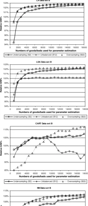
Stage 3 considered the joint effect of varying the sample size and balancing in combination.Fig. 3shows the relative performances of LR, LDA, CART and NN for undersampling (B2), the unbalanced data set (B12) and oversampling (B13)

for increasing sample sizes.

Fig. 3displays a number of features. The first is that the sample size clearly has an effect on the relative performances of different balancings. In particular, for smaller sample sizes, undersampling performs poorly across both data sets for LR, LDA and NN. The relative performance of undersampling compared to oversampling shows a monotonic increasing trend as the sample size increases, until the difference in performance for LR, LDA and NN becomes small for the largest samples. However, at no point does undersampling ever outperform oversampling for these three methods. In addition, for NN and LR, undersampling marginally underperforms the unbalanced data set for all sample sizes. For LDA, the

(12)

a

b

Fig. 2. Absolute model performances for datasetsA(a) andB(b) using all available data (p=100).

story is somewhat different. In general, oversampling outperforms the unbalanced data set, but for smaller sample sizes, undersampling performs poorly once again. CART shows the most divergent behaviour between methods. In particular, the best method for balancing the data appears to be very dependent upon the sample size. For small sample sizes, undersampling performs well, but the performance of oversampling relative to that of undersampling increases monotonically as the sample size increases, until a point is reached at which the situation is reversed, with oversampling being superior for larger samples.

5. Conclusions and discussion

This paper has addressed two issues, sample size and balancing. For the sample size, the position adopted in practice by many scorecard developers is that a sample containing around 1500–2000 cases of each class (includ-ing any holdout sample) is sufficient for build(includ-ing and val-idating a credit scoring model which is nearly optimal in terms of predictive performance. The results presented in this paper undermine this view, having demonstrated that there are significant benefits from taking samples many times larger than this. As a consequence, the paper chal-lenges current beliefs by suggesting the use of significantly larger samples then those commonly used in credit scoring practice and academic studies, even for the well researched LR, contributing to the current discussion on data prepro-cessing and modelling for credit scoring.

A further issue in relation to the sample size relates to the relative efficiency of algorithms. The results presented in this paper support the case that efficient modelling techniques, such logistic regression, obtain near a optimal performance using far fewer observations than methods such as CART and NN. Therefore, the sample size should be considered when deciding which modelling technique to apply.

Another practice which is widely adopted by scorecard developers is undersampling. Equal numbers of goods and bads are used (by excluding instances of the majority class of goods) for model development, with weighting being applied so that the performance metrics are representative of the true population. Our experiments provide evidence that oversampling significantly increases the accuracy relative to undersampling, across all algorithms, a novel insight which confirms prior research in data mining for imbalanced credit scoring datasets (albeit at the cost of larger datasets and longer training times, and hence reduced resource efficiency). For logistic regression, the most popular technique used for constructing credit scoring models in practice, the balancing applied to datasets appears to be of minor importance (at least for modestly imbalanced data sets such as the ones discussed in this paper). However, the other methods demonstrate a greater sensitivity to balancing, particularly LDA and CART, where oversampling should be considered as the new best practice in assessing them as contender models to LR.

The results hold across two datasets in credit and behavioural scoring, indicating some level of consistency of the results. Here, the choice of two heterogeneous datasets reflects an attempt to assess the validity of the findings across different data conditions, rather than an attempt to increase the reliability. However, while one should be careful to generalise experimental findings beyond the properties of an empirical dataset, credit scoring datasets are remarkably similar across lenders and geography, and might yield more representative results if controlling for the sample size and balance. However, in the absence of additional datasets of sufficient size, the obvious limitations of any empirical ex-post experiment remain.

With regard to further research, there are a number of avenues for further study. One area is the application of active learning (Cohn, Atlas, & Ladner, 1994;Hasenjager & Ritter, 1998), by selecting cases of imbalanced classes that provide a better representation of both sides of the prob-lem domain during the parameterisation phase, promis-ing smaller samples with similar levels of performance to those of larger random samples. Also, there is evidence that instance sampling may have interactions with other pre-processing choices which occur prior to modelling (Crone et al., 2006). Consequently, popular techniques in credit scoring which employ, for example, weights of evidence (Hand & Henley, 1997;Thomas,2000), instead of the pure dummy variable categorization evaluated here, must be evaluated on different forms of over- and undersampling.

The conclusions drawn from the experiments in in-stance sampling have implications for previous research findings. In general, previous studies in credit scoring have not reflected the recommendations employed in practice,

(13)

Fig. 3. Effect of balancing in combination with sample size.

evaluating small and imbalanced datasets, which calls into question the validity and reliability of their findings on real-world datasets. Replication studies which re-evaluate these empirical findings across different sampling strate-gies may resolve this discrepancy. Similarly, the relatively few academic studies of sub-population modelling applied to credit scoring have come to somewhat mixed

conclu-sions, yet the practice is widely accepted in industry, where it is more common to employ larger samples. Considering the smaller sample sizes employed across most academic studies, our research would identify this as a limiting factor which could also explain why sub-population models have failed to show better levels of performance than might have been expected (see e.g. Banasik, Crook, & Thomas,