Technological University Dublin
Technological University Dublin
ARROW@TU Dublin
ARROW@TU Dublin
Articles
School of Computing
2013
Using Semi-supervised Classifiers for Credit Scoring
Using Semi-supervised Classifiers for Credit Scoring
Kenneth Kennedy
Technological University Dublin, [email protected]
Brian Mac Namee
Technological University Dublin, [email protected]
Sarah Jane Delany
Technological University Dublin, [email protected]
Follow this and additional works at: https://arrow.tudublin.ie/scschcomart Part of the Computer Sciences Commons
Recommended Citation
Recommended Citation
Kennedy, K., MacNamee, B. &Delany, S. (2013) Using Semi-supervised Classifiers for Credit Scoring. Journal of the Operational Research Society,vol. 64, pp.513-529. doi:10.1057/jors.2011.30
This Article is brought to you for free and open access by the School of Computing at ARROW@TU Dublin. It has been accepted for inclusion in Articles by an authorized administrator of ARROW@TU Dublin. For more
information, please contact
[email protected], [email protected], [email protected].
This work is licensed under a Creative Commons Attribution-Noncommercial-Share Alike 3.0 License
Using semi-supervised classifiers for credit scoring (Accepted for Publication)
K. Kennedya,∗, B. Mac Nameea, S.J. DelanybaSchool of Computing, Dublin Institute of Technology, Ireland bDigital Media Centre, Dublin Institute of Technology, Ireland
Abstract
In credit scoring, low-default portfolios are those for which very little default history exists. This makes it problem-atic for financial institutions to estimate a reliable probability of a customer defaulting on a loan. Banking regulation (Basel II Capital Accord), and best practice, however, necessitate an accurate and valid estimate of the probability of default. In this article the suitability of semi-supervised one-class classification algorithms as a solution to the low-default portfolio problem are evaluated. The performance of one-class classification algorithms is compared with the performance of supervised two-class classification algorithms. This study also investigates the suitability of oversam-pling, which is a common approach to dealing with low-default portfolios. Assessment of the performance of one-and two-class classification algorithms using nine real-world banking data sets, which have been modified to replicate low-default portfolios, is provided. Our results demonstrate that only in the near or complete absence of defaulters should semi-supervised one-class classification algorithms be used instead of supervised two-class classification al-gorithms. Furthermore, we demonstrate for data sets whose class labels are unevenly distributed that optimising the threshold value on classifier output yields, in many cases, an improvement in classification performance. Finally, our results suggest that oversampling produces no overall improvement to the best performing two-class classification algorithms.
Keywords: banking, credit scoring, low-default portfolio, supervised classification, one-class classification, benchmarking
1. Introduction
The upheaval in the financial markets that accompanied the sub-prime mortgage crisis has emphasised the large proportion of the banking industry based on consumer lending (Thomas, 2009). Credit scoring is an important part of the consumer lending process that attempts to predict the repayment behaviour of borrowers. It is an endeavour regarded as one of the most important application fields for both data mining and OR techniques (Baesenset al., 2009). The objective is to assign borrowers to one of two groups: goodor bad. A member of the goodgroup is considered likely to repay their financial obligation. A member of thebadgroup is considered likely to default on their financial obligation.
Generally, credit scoring models are categorised into two different types, application scoringandbehavioural scoring. Application scoring attempts to predict a customer’s default risk at the time an application for credit is made based on information such as applicant characteristics and credit bureau records. Behavioural scoring assesses the risk of existing customers based on their recent accounting transactions. In this paper, we focus on application scoring due to the availability of suitable data sets. The techniques we describe and our findings, however, could equally apply to behavioural scoring.
Under the Basel II Capital Accord (BCBS, 2005a), using the internal ratings-based approach, banks can calculate their capital requirements by using their internal data to construct credit risk models. As a consequence of this approach greater emphasis is placed on an accurate estimation of customers’probability of default(PD) rather than
∗
Correspondence: Kenneth Kennedy, K107A, School of Computing, Dublin Institute of Technology, Kevin St., D8, Ireland Email address:[email protected](K. Kennedy)
the ability to correctly rank customers based on their default risk (Malik and Thomas, 2010). PD also has to be predicted not just at an individual level but also for segments of the loan portfolio. Modelling the PD is essentially a discrimination problem (good or bad), consequently one may resort to the numerous classification techniques that have been suggested in the literature. Many of these classification models are derived from statistical methods, non-parametric methods, and artificial intelligence approaches.
At certain stages of an economic cycle the number of defaulters can be very low, which complicates the modelling process. It is well known that the performance of standard supervised classification techniques deteriorates in the presence ofimbalanced data(Chawlaet al., 2010). Imbalanced data refers to a situation where one class is under-represented compared to the other class. This imbalance may be due to two reasons. The first is that the proportion of one class in the sample is lower than the proportion in the population. The second is that in both the sample and population the proportion of one class differs from the other. In this paper we are interested in assessing the latter as it can affect classifier training, for example an increase in the variation of the coefficients obtained by logistic regression (Hand and Henley, 1993). In credit scoring imbalanced data is common due to the usual absence of defaulters and this is known as thelow-default portfolio problem. Even in the current financial crisis low-default portfolios are the norm - for the second quarter of 2010, the Council of Mortgage Lenders, UK, reported that the number of mortgages three or more months in arrears stood at 2.17% of total outstanding mortgages (CML, 2010).
One possible approach to addressing the low-default portfolio problem is the use ofone-class classification(OCC) algorithms (also known asoutlier detection). OCC has attracted much attention in the data mining community (Chawla et al., 2004). It is a recognition-based methodology that draws from a single class of examples to identify thenormal or expected behaviour of a concept. This is in contrast to standard supervised classification techniques that use a discrimination-based methodology to distinguish between examples of different classes.
In this article we compare one-class classification methods with more common two-class classification approaches on a number of credit scoring data sets, over a range of class imbalance ratios. As a means for handling imbalanced data we oversample the minority class along with adjusting the threshold value on classifier output. The purpose of this study is to determine whether or not the performance of OCC methods warrants their inclusion as an approach to addressing the low-default portfolio (LDP) problem. To the best of our knowledge, no attempt has been made to examine OCC as a solution to the LDP problem before.
The comparative assessment of classification methods can be a subjective exercise. It is influenced, amongst other factors, by the expertise of the user with each of the methods used and the effort invested in refining and optimising each method (Hand and Zhou, 2009; Thomas, 2009). We attempt to overcome this problem by restricting our study to a single application area (low-default portfolios); by selecting appropriate performance measures (Hmeasure and harmonic mean); and finally by using nine different data sets of varying size and dimension to capture as many as possible of the particular aspects of the LDP problem.
The remainder of this article is organised as follows. A review of the relevant literature is provided in Section 2. The two-class and one-class classification algorithms used in the study are covered in Section 3. Section 4 describes the experimental methodology, and Section 5 presents experimental results. Section 6 discusses conclusions and directions for future work.
2. The low-default portfolio problem: previous work
The introduction and implementation of the Basel II Capital Accord (BCBS, 2005a) has had a major impact on credit scoring. Regulation stipulates that banks must set aside adequate capital buffers to withstand losses and sustain lending during unanticipated turbulence in the economic environment. Regulating the minimum capital buffer, or regulatory capital, is a primary area of interest for banking supervision (Ingolfsson and Elvarsson, 2010). Basel II allows banks to adopt aninternal ratings-based(IRB) approach to regulatory capital. This allows banks to calculate their regulatory capital based on their own assessment of key risk components, including the PD which is considered to be the likelihood that a borrower will default in the next 12 months. The PD is the“central measurable concept on which the IRB approach is built”(BCBS, 2001). Normally the PD is calibrated using an internal data source with a sufficient history (e.g. 5+years) to which a score function, such as logistic regression, is applied. The PD is calculated yearly counting defaults versus non-defaults and averaging.
To use the IRB approach, lenders must be able to build models that are validated to have consistent and accurate predictive capacity (BCBS, 2005a, Paragraph 500). This has raised concern in the financial industry that institutions
with low-default portfolios may be excluded from the IRB approach due to inability to build and validate accurate models (BBA, 2004). As a consequence such institutions would be forced to use simpler approaches requiring greater amounts of regulatory capital.
Many of the papers addressing the LDP problem do not investigate the issue of comparing the predictive per-formance of classification models through out-of-sample testing. Focus is instead given to the application of various statistical techniques that attempt to bolster the information generated by the monotonic ordering of the portfolio or by the small number of defaults in the portfolio. Such papers are concerned with the accurate model validation of LDPs. Some of the more well known works include Pluto and Tasche (2006) who address the LDP problem by proposing the “most prudent estimation principle”. This approach relies on the assumption that the ordinal ranking of the borrowers, who are split into grades of decreasing credit-worthiness, is correct. Forrest (2005) adopted a similar method to Pluto and Tasche (2006), but in contrast this method is based on a likelihood approach working in multiple dimensions, where each dimension corresponds to a rating grade and each point represents a possible choice of grade-level PDs.
Overall, the two main technical challenges presented by LDPs are: (i) estimating an accurate PD when no historical defaults are available; and (ii) assessing a model’s predictive performance (Stefanescuet al., 2009). Both of these issues arise not only during the validation of the model, but also prior to this, during the construction of the model. In this article we are concerned primarily with model construction and the comparison of the predictive performance of classification models. In many of the works addressing the LDP problem, the construction of the model is dependent on: (i) making assumptions about the ordering of the data; (ii) incorporating expert opinion; or (iii) the availability of a certain number of historical defaults generated either artificially or occurring in reality.
Given one of these dependencies, the models constructed are typically either: (i) statistical models constructed from a representative pool of data; or (ii) expert systems (or knowledge-based approaches) whose parameters are determined by financial experts. van Gestel and Baesens (2009) highlight several experimental studies from various domains which conclude that quantitative statistical models outperform human experts (e.g. Meehl, 1955). This is not to say that certain knowledge-based approaches, (e.g. fuzzy classification rules) cannot be successfully utilised to achieve good predictive ability amongst loan applicants (Tang and Chi, 2005). Indeed, an advantage of such approaches is the ability to generate explanatory models which provide the expert with an explanation as to why a certain credit applicant is accepted or rejected (Hoffmannet al., 2007). However, such systems are beyond the scope of this article in which we focus on quantitative approaches. The two main types of statistical models areduration modelsandclassification models. Duration models focus on the time to default and rely on a large data set (Medema et al., 2009). Much research has been conducted on adapting classification techniques to construct credit scoring models. Such classification techniques and studies include: (i) traditional statistical methods such as; discriminant analysis (Eisenbeis, 1977) and logistic regression (Westgaard and van der Wijst, 2001), (ii) non-parametric statistical methods: for example,k-nearest neighbour (Henley and Hand, 1996), (iii) decision trees (Quinlan, 1993); and (iv) neural networks (West, 2000). Additional techniques include support vector machines (Schebesch and Stecking, 2005), genetic algorithms (Desaiet al., 1997), and ant colony optimisation (Martenset al., 2009). It is possible to combine many of these methods to create an ensemble classification technique. Much of this research is performed on the basis that the constructed credit scoring models use data sets containing a representative number of historical defaults. The LDP problem is not assessed.
The question of which classification technique to select for credit scoring remains a complex and challenging problem. Baesenset al.(2003) highlight the confusion resulting from comparing conflicting studies. Some studies may recommend one particular classification algorithm over another, whilst other studies recommend the opposite. Furthermore, many of these studies evaluate a limited number of classification techniques, restricted to a small num-ber of credit scoring data sets. To compound this, many of the data sets are not publicly available, thus curtailing reproducibility and verifiability. Another problem is authors’ expertise in their own method and failure to undertake a corresponding effort with existing methods (Michieet al., 1994). Indeed, Thomas (2009) highlights that studies which have endeavoured to avoid the aforementioned problems (Baesenset al., 2003; Xiaoet al., 2006) have reported that the differences between the performance of classification techniques were small and regularly not statistically significant. Great care and consideration was taken to avoid these issues in this work, details of which are given in Section 4.
To the best of our knowledge a benchmarking study of the performance of classification techniques on low-default portfolios has not been described in the literature. Indeed, a comparative study of one-class classifiers used in the context of credit scoring has not been described in the literature. The most closely related, work to this is
Juszczaket al.(2008), which describes a comparison of one- and two-class classification algorithms used for detecting fraudulent plastic card transactions. The results of that study found that two-class classifiers will outperform one-class classifiers - provided that the training and test objects are from the same distribution. Plastic card fraud detection is also examined by Krivko (2010) who provide a framework for combining one- and two-class classifiers to identify fraudulent activity on debit card transaction data. The following section will introduce the classification techniques used in this study.
3. Classification techniques
Insupervised classificationa model is induced from a set of labelled data examples. Previously unseen examples are then assigned to one of the classes learnt by the model. In this article we compare eight well-known supervised classification methods that are suitable for credit scoring and require minimal parameter tuning: Fisher’s Linear Discriminant Analysis (LDA) (see Webb, 2002), Linear Bayes Normal (LDC) (see Duda and Hart, 1973), Quadratic Bayes Normal (QDA) (see Duda and Hart, 1973), Logistic Regression (LOG) (see Hosmer and Lemeshow, 2000), Na¨ıve Bayes Kernel Estimation (NB) (see Hand and Yu, 2001), Support Vector Machines (SVM) Vapnik (1995), Neural Network Back Propagation Feed-Forward Network (NN) (see Bishop, 1995), andk-Nearest Neighbour (k -NN) (see Henley and Hand, 1996). The OCC techniques used are less well known and so are covered in greater detail.
OCC techniques distinguish a set of target objects from all other objects (Moya et al., 1993). This is a form ofsemi-supervised classification as the training data consists of labelled examples for the target class only. OCC techniques have been applied to a wide range of real-world problems such as machine fault detection (Sarmiento et al., 2005), fraud detection (Juszczaket al., 2008), and identity verification (Hempstalk, 2009). The term OCC is believed to have originated from Moyaet al.(1993) and is only one of a number of terms used to describe similar approaches - other terms includeoutlier detection(Ritter and Gallegos, 1997),novelty detection(Bishop, 1994), and concept learning(Japkowicz, 1999).
Following the taxonomy described by Tax (2001), OCC techniques can be divided into three groups: density methods,boundary methods, and reconstruction methods. This is by no means an exhaustive discrimination, but conceptually it is the simplest and most popular. For a detailed description of OCC taxonomies refer to (Chandola et al., 2009).
All OCC methods share two common elements: a measure of the proximity of an object,z, to the target data; and a threshold,θ, to which the proximity measure is compared. An object,z, is considered to be a member of the target class when the proximity ofzto the target data is less than the thresholdθ.
Density estimation approaches to OCC directly estimate the probability distributions of features for the target class by fitting a statistical distribution, such as Gaussian, to the target data. The success of this approach depends on factors such as the target data sample size and whether the selected statistical distribution is appropriate for the target data. The density techniques provide the most complete description of the target data, but as a drawback to this they may require large amounts of data (Tax and Duin, 1999).
OCC approaches based on boundary estimation fit a boundary around the target class data, whilst simultaneously attempting to minimise the volume of the enclosed area. Boundary methods offer a degree of flexibility in that an estimate of the complete probability density is not necessary. The computation of the boundary is based on the distances between the objects in the target data. In some cases a kernel function is used to define a flexible boundary. This approach works well with small sample sizes and an uncharacteristic training data set (Tax, 2001).
Reconstruction methods are trained to reproduce an input pattern by assuming a model of the data generation process. The parameters of the assumed data generation model are estimated during the learning phase. This differs from density and boundary methods as reconstruction methods do not rely on statistical assumptions made about the data. A reconstruction error is used to determine if the object belongs to the target or outlier class.
A good OCC model should maximise both the number of target objects accepted and outlier objects rejected. Specifying the trade-off between the fraction of target objects accepted and the fraction of outlier objects rejected ,through the thresholdθis the most important feature of OCC (Tax, 2001). The threshold is usually adjusted heuristi-cally (and evaluated using a test data set) to attain the desired trade-off. Too small a value forθwill cause the model to underfit the data and cover the entire feature space, whereas a largeθwill over-fit the data, resulting in a minimised target space.
In some circumstances certain OCC models can incorporate outlier data. The performance of a OCC model may be compromised if outlier data is used as the performance of the model becomes dependent on the outlier data and poor quality data or low quantities of outlier data which are not representative of the problem will damage performance (Hempstalk, 2009). For clarity such models are not used in this study although they may be considered in future work. The remainder of this section will describe each of the OCC algorithms used in our evaluations (in all cases the actual implementation used is from the Matlab Data Description Toolbox (DDTools) (Tax, 2009) and some specific details given stem from this).
Gaussian (Gauss):A density estimation method that assumes the target data is generated from a unimodal
multivari-ate normal distribution, the Gaussian model is one of the simplest OCC techniques (see Tax, 2001). For an object,z, the Mahalanobis distance to the training set distribution is calculated as follows:
f(z)=(z−µ)TΣ−1(z−µ) (1) where µ is the mean and Σ is the covariance matrix of the training set, both of which are estimated using an Expectation-Maximisation (EM) approach. This distance is compaed to a thresholdθto make a classification. The Mahalanobis distance is used in order to avoid numerical instabilities. A caution to the use of the Gaussian method is that if the assumption that the data fits a normal distribution is violated the model may introduce a large bias (Tax, 2001).
Mixture of Gaussians (MOG):A mixture of Gaussians model (see Bishop, 1995) is a linear combination ofkGaussian
distributions. Although this is a more flexible approach than the single Gaussian method it requires more data as it may display greater variance when only a limited amount of data is available. To build a mixture of gaussians model the training data is divided intokclusters, each of which is modelled by a Gaussian distribution. For an objectza superposition ofkGaussian densities can be written as:
f(z)= k X i=1 αiexp n −(z−µi)TΣi−1(z−µi)o (2)
whereαiare the mixing coefficients, againµis the mean andΣis the covariance matrix. For each clusteri,αi,µiand Σiare estimated using the EM algorithm. Given a mixture, the threshold,θon the density determines ifzis classified
as target or non-target data.
Parzen Density Estimation (Parzen): The Parzen density estimator (Parzen, 1962) is an extension of the mixture of
Gaussians method. It is a non-parametric technique that uses a kernel to estimate the probability density function. Each object in the target class is treated as the centre of a Gaussian distribution. Based on this, a measure of the likelihood that an object belongs to the target data is computed by averaging the probability of membership of the Gaussian distributions. Classification is obtained by comparison to a threshold,θ. Letp(z) be the density function to be estimated. Given a setD={z1,z2. . .zn}ofntarget objects, the Parzen density estimate of p(z) is:
p(z)= 1 nh n X i=1 ρz−zi h (3)
wherehis a smoothing parameter, andρis typically a Gaussian kernel function: ρ(z)= √1
2πe
−1
2z2 (4)
The width of the Gaussian kernel,h, is optimised by maximising the likelihood in a leave-one-out fashion, as per Kraaijveld and Duin (1991).
When large differences in density exist, the Parzen kernel method will give poor results in low density areas. Like all density approaches, it requires a large amount of target data to make a reliable probability density estimation.
Na¨ıve Parzen (NParzen): The na¨ıve Parzen is a simplification of the Parzen density estimator inspired by the na¨ıve
Bayes approach (see Hastieet al., 2005). A Parzen density is estimated in each feature dimension separately, and the probabilities are multiplied to give the final target probability.
k-Nearest Neighbour (k-NN):Thek-nearest neighbour (Cover and Hart, 1967) method can be adopted to construct a one-class classifier. The one-classk-NN (Tax and Duin, 2000) classifier is a boundary-based approach that is based on the number of target objects in a region of a certain volume. Classification is performed using a threshold on the ratio between two distances. The first is the distance between the test objectzand itskth nearest neighbour in the training set,NN(zi,k) (kis a parameter of the approach). The second distance is measured as the distance between the
kth nearest training object and itskth nearest neighbour. The ratio is calculated as follows: p(z)= k(z,NN(z,k))k
k(NN(z,k),NN(NN(z,k),k))k (5)
where Euclidean distance is used to measure the distance between objects. For further details refer to Tax (2001).
Support Vector Domain Description (SVDD):The SVDD (Tax and Duin, 1999) is a kernel-based boundary method
which attempts to find the most compact hypersphere that encloses as many target instances as possible. By minimis-ing the volume of the hypersphere, the chance of acceptminimis-ing outlier objects is reduced. To generate a flexible boundary the input space can be mapped into a higher dimensional and more separable feature space. This transformation is typically performed using a Gaussian kernel. Classification is performed by comparing the distance between an object,z, and the target boundary to a threshold,θ.
k-Means: k-Means clustering (see Bishop, 1995) can be adapted into a relatively straight-forward reconstruction
approach to OCC. The approach subdivides the output space, onto which new objects are projected, intokcluster prototypes or centres. The prototypes are located such that the average distance to a prototype centre is minimised as follows:
k−means=Σ
i(minkkzi−µkk2) (6)whereµkrepresents thek-th cluster centre. The objects in the training set are clustered, and when a new object is to
be classified its distance from the nearest prototype is used as a measure that can be thresholded in order to identify outliers. If the distance is greater than a threshold,θ, the object will be classed as non-target data. A drawback can be that outliers form in clusters by themselves.
Auto-encoders (AE): Anauto-encoder, also referred to as an auto-associator, is a reconstruction based approach
introduced by Japkowicz (1999) based on the work of Hinton (1989). An auto-encoder is a particular type of neural network, which is trained to reproduce an input patternXat the output of the network,NN(X). Because the network has a narrow hidden layer (orbottleneck), it compresses redundancies in the input. This feature can be utilised to train the network to reconstruct examples from a target class as accurately as possible. Such a network will then perform poorly at reconstructing non-target data which present different structural irregularities. Classification is achieved by comparing the reconstruction error when test examples are presented to the network to a threshold.
The next section will explain the experimental methodology used to compare the performance of these classifica-tion algorithms in an LDP scenario.
4. Evaluation experiment
The aims of this evaluation described are to examine the effectiveness of oversampling and the use of one-class classification in addressing the LDP problem. This is achieved by comparing the performance of one-class classifiers to that of two-class classifiers. Furthermore, we investigate to what extent optimising the threshold value on classifier output yields an improvement in classification performance. To accomplish the above aims we adopt three separate approaches:
(i) Classifying an imbalanced data set using a selection of two-class classifiers.
(ii) Oversample the minority class of the data set and employ a selection of two-class classifiers. (iii) Remove the minority class completely and use one-class classification.
The first two approaches compare various two-class classifiers on credit scoring data sets with different degrees of class imbalance. Both approaches illustrate the adverse consequences of class imbalance. Based on the results of (i) and (ii) the best performing two-class classifier is then used in approach (iii) where its performance is compared to a selection of one-class classifiers on the same data sets but with a greater degree of class imbalance. This section describes the data sets, performance measures and methodology used.
4.1. Data sets
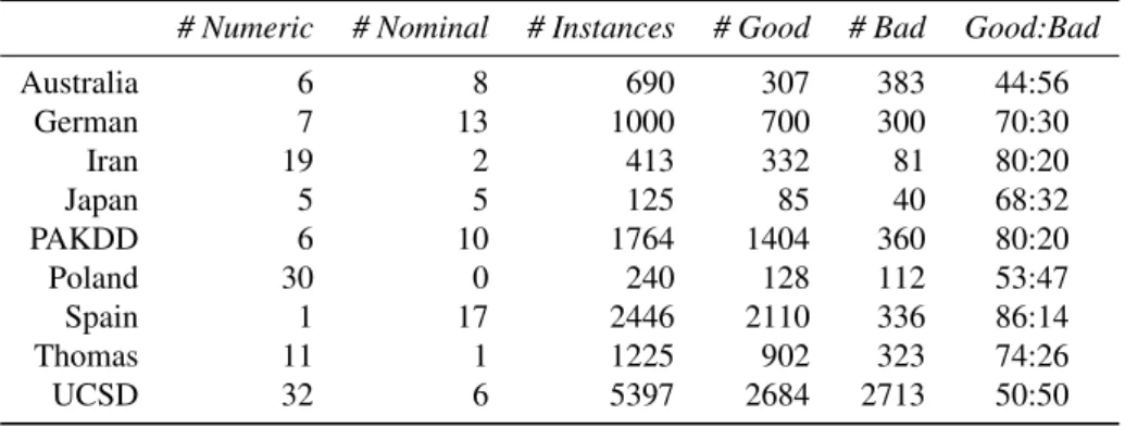
The characteristics of the nine data sets used are presented in Table 1. The Australia, German and Japan credit data sets are publicly available at the UCI Machine Learning repository (http://archive.ics.uci.edu/ml/datasets.html). The Japan data set is commonly mistaken for the Australia data set, for example, by Tsai and Wu (2008) and Nanni and Lumini (2009). The Iran data set is an updated version of a data set that appears in Sabzevariet al.(2007). It consists of corporate client data from a small private bank in Iran. The Poland data set contains bankruptcy information of Polish companies recorded over a two-year period (Pietruszkiewicz, 2008). The Spain data set compiled by Dionne et al.(1996) comes from a large Spanish bank and details personal loan applicants. The Thomas data set is a CD ROM accessory of Thomaset al.(2002) describing applicants for a credit product. Two of the original fourteen features have been removed due to incomplete records. The Pacific-Asia Knowledge Discovery and Data Mining conference (PAKDD) data set is a modified version of the PAKDD 2009 competition data set. We removed redundant features and in order to reduce the size of the data set we limit our selection of instances based on four differentphone code feature values. The University College of San Diego (UCSD) set is also a modified competition data set used in the 2007 University College of San Diego/Fair Issac Corporation (UCSD/FICO) data mining contest. We randomly undersampled both classes to reduce the size of the data set and removed redundant identity features.
Table 1: Characteristics of the nine data sets used in the evaluation experiment.
# Numeric # Nominal # Instances # Good # Bad Good:Bad
Australia 6 8 690 307 383 44:56 German 7 13 1000 700 300 70:30 Iran 19 2 413 332 81 80:20 Japan 5 5 125 85 40 68:32 PAKDD 6 10 1764 1404 360 80:20 Poland 30 0 240 128 112 53:47 Spain 1 17 2446 2110 336 86:14 Thomas 11 1 1225 902 323 74:26 UCSD 32 6 5397 2684 2713 50:50
All numerical attributes are normalised to values between 0 and 1 by applying min-max range normalisation. The sample sizes vary considerably from 125 to 5,397 instances. Although commercially used scorecards are usually constructed from an initial sample size of between 10,000 and 50,000 (Thomas, 2009), the above data sets are all easily available in public literature whereas many other data sets used in credit scoring studies are privately held and cannot be shared amongst researchers. As per Keogh (2007), we believe that the irreproducibility of results caused by, amongst other things, the refusal to share data or to give parameter settings hinders the research process. To ensure reproducibility of the contents of this paper, we have provided access to all of the data and developed techniques used in this article at: http://www.comp.dit.ie/aigroup/jorsCreditScoringCode.zip.
4.2. Evaluation measures
Two evaluation measures are used in this study: the harmonic mean and the Hmeasure. The harmonic mean measures classification performance at a specific classification threshold, whereas theHmeasure assesses classifier performance over a distribution of costs. Differences between the performance of various techniques were analysed with a Friedman test (Friedman, 1937) with post hoc pairwise comparisons performed with a Holm’s procedure (Holm, 1979) (all tests testing for significance were at the 5% level). The remainder of this section will describe the two measures used.
4.2.1. Harmonic mean
Classifier output is typically binary: 1 for accepting (non-defaulter) or 0 for rejecting (defaulter) a credit applicant. Many ranking classifiers also produce a numeric score which can be binarised by the use of a threshold. The threshold determines true positive (TP), true negative (TN), false positive (FP) (classified as positive, but actually negative) and
false negative (FN) (classified as negative, but actually positive) counts for a given test set. We useSensitivity and Specificity, as used by Baesenset al.(2003), to measure the classification quality of all classifiers used in our study. Sensitivity is calculated as: T P
T P+FN and measures the proportion of positive (non-default) examples that are predicted
to be positive. Specificity, calculated as: T NT N+FP, measures the proportion of negative (default) examples that are predicted to be negative. As per Hoffet al.(2008), in order to provide a suitable composite measure of sensitivity and specificity we employ theharmonic mean, which is calculated as shown in Equation 7.
Harmonic Mean= 2∗Sensitivity∗Specificity
Sensitivity+Specificity (7)
Lessmannet al. (2008) opted out of selecting a classification threshold contending that studies comparing the same classifiers and data sets could easily come to different conclusions as a result of employing different methods for determining classification thresholds. We address this issue by clearly defining the harmonic mean. It assumes equal misclassification costs for both false positive and false negative predictions. This may be a problem if we consider that one type of classification error may be a lot more costly than the other. However, in the absence of available cost matrices the harmonic mean is the most appropriate performance criteria as a means of assessing the accuracy of a classifier at a specific threshold.
4.2.2. H measure
The Kolmogorov-Smirnov statistic, the Gini coefficient and the AUC are commonly used in credit scoring to estimate the performance of classification algorithms in the absence of information on the cost of different error types. Hand (2009), however, demonstrates how these measures actually use costs derived from the data used and suggests that their application may produce misleading results about classification performance. For example, the AUC uses a probability distribution of the likely cost values that depend on the actual score distributions of the classifier. As a result the probability distribution of the likely cost values will vary from classifier to classifier, as per the score distribution. This prevents different classifiers from being compared in an equal manner.
As an alternative, Hand proposes theH measure (Hand, 2009) that uses a probability distribution of the likely cost values that is independent of the data. ThisBetadistribution (see Hand, 2009) contains two parameters,αandβ that can increase the probability on certain ranges of the cost believed to be more likely. It is recommended that for situations when nothing is known about the costs then a Beta distribution withα=2 andβ=2 should be used. In this study we adopt the recommendedαandβsettings so as to allow for universally comparable results.
4.3. Methodology
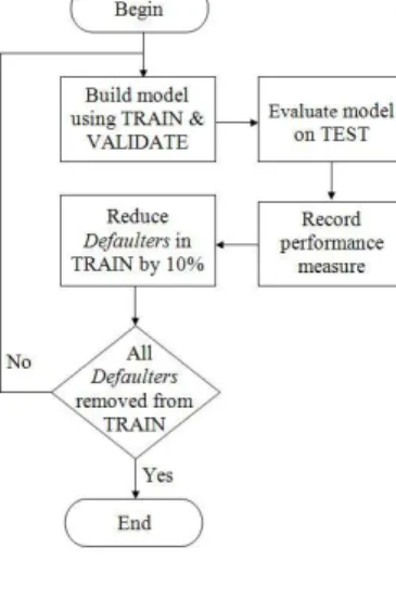
Each data set used was divided into three subsets: (i) the training set (55%); (ii) the validation set (15%), and (iii) the test set (30%). The training set and the validation set were used to train and tune the classifiers while the test set was used to verify their performance. This procedure was performed repeatedly over a number of turns. At the end of each turn the number of instances in the defaulter class of the training set was reduced by 10%. The model was then retrained and retuned using the training and the validation sets. Figure 1 illustrates this process which we refer to as thenormal process.
We conduct a second set of experiments on the same data sets whereby we oversample the number of instances from the defaulter class. This process was similar to the normal process except that after reducing the instances in the defaulter class of the training set by 10% the remaining defaulter class instances were oversampled to produce a balanced training set. This oversampling occurs in the training data only. The validation set and the test set remain unchanged. We call this theoversample process, Figure 2 illustrates the procedure.
Finally, a third set of experiments using one-class classifiers is performed. To perform OCC we remove all the instances of the defaulter class from the training set, so that only instances from the non-defaulter class are used to build the model. Again, the validation set and testing set remain unchanged. We call this process theone-class classification process(OCC process).
In all three groups each experiment was conducted 10 times using different randomly selected training, test and validation set splits and the results reported are averages of these 10 runs.
Figure 1: Normal process; training set - TRAIN, validation set - VALIDATE, test set - TEST.
4.4. Classifier tuning
The parameter settings for each classifier used are based on best practice. The na¨ıve Bayes, linear Bayes normal and Fisher’s linear discriminant analysis supervised classifiers require no parameter tuning. For the quadratic Bayes normal classifier, the regularisation parameters used to obtain the covariance matrix were optimised using the vali-dation set. For the neural network the number of hidden layers was fixed at 1 and the number of units in the hidden layer matched the dimensionality of the input space, as per Piramuthu (1999). Thek-NN classifier usesk=10 and Euclidean distance to determine the similarity between instances. For the logistic regression classifier the number of cross validation iterations used to obtain the optimal feature class weights is optimised between 1 and 20 using the validation set. The SVM classifier uses a linear kernel and the cost function parameter is fixed at 0.5. The linear Bayes normal, Fisher’s linear discriminant analysis, neural network, and quadratic Bayes normal supervised classifiers were implemented using PrTools (Duinet al., 2008). Thek-NN, logistic regression, and na¨ıve Bayes supervised classifiers were implemented in the Weka (version 3.7.1) machine learning framework (Witten and Frank, 2000). The SVM clasifier was implemented using LibSVM (Chang and Lin, 2001).
The class classifiers were implemented using the Matlab DDTools toolbox (Tax, 2009). For the Gaussian one-class one-classifier the regularisation added to the estimated covariance matrix is optimised using the validation set. For the mixture of Gaussians, the number of clusters containing defaulters is optimised between 1 and 3 using the validation set. For each cluster the full covariance matrix was calculated. The regularisation for the covariance matrices was optimised using the validation set. For both thek-Means andk-NN classifierskwas set at 10. Both the Parzen and na¨ıve Parzen used automated parameter settings. For the Auto-encoder the number of hidden layers was fixed at 1 (the default value). The number of hidden units was set to 5 (the default setting). With the SVDD, the parameter controlling the tightness of the boundary,σ, was optimised between 1 and 12 using the validation set.
The next section will describe the results of this experimental process.
5. Results
Figure 3 illustrates the resultingHmeasure when eight two-class classifiers using the normal process and eight one-class classifiers using the OCC process were tested on the Australia data set. The horizontal axis represents the percentage of defaulters present in the training data set. The two-class classifiers are identifiable by their deteriorating performance caused by the gradual removal of defaulters from the training data set. As the number of non-defaulters used to train the one-class classifiers is fixed, the performance of the one-class classifiers remains static throughout. Due to space restrictions, we only display results for the Australia data set as the pattern shown is similar for all datasets.
Three separate segments have been highlighted in Figure 3, each representing a level of class imbalance (70:30, 80:20, and 90:10) at which we compare the performance of two-class classifiers. For some data sets (e.g. Spain) the initial level of imbalance only allows the two-class classifiers to be compared at class imbalances of 80:20 or 90:10. 5.1. Two-class classifier performance with imbalance
The effects of class imbalance using the normal process are clearly evident in Figure 3. Beginning with a class imbalance of 44:56 (44% non-defaulter, 56% defaulter) the performance of the two-class classifiers gradually deteri-orates as the class imbalance increases through the removal of instances from the defaulter class in the training set. The performance of the na¨ıve Bayes and logistic regression classifiers remains relatively robust while, in contrast, the performance of the Lin SVM,k-NN and NN classifiers deteriorates rather more rapidly. So that more general comparisons can be made Table 2 shows theH measure for each two-class classifier at imbalance ratios of 70:30, 80:20, and 90:10 for the nine data sets used.
Figure 3: Normal process and one-class classification process test setHmeasure performance. Selected class imbalance ratios are also highlighted at 70:30, 80:20 and 90:10.
T able 2: T est set H measure performance using the normal process on tw o-class classifiers. The best test set H measure at each class imbalance ratio is underlined. The rank of the di ff erent classifiers at each class imbalance ratio is av eraged o v er all the data sets and reported as the AR (a v erage rank). H measure figures should be multiplied by 10 − 2 . Tec hnique Austr alia German Poland UCSD Ir an Japan PAKDD Thomas Spain AR 70:30 80:20 90:10 70:30 80:20 90:10 70:30 80:20 90:10 70:30 80:20 90:10 80:20 90:10 80:20 90:10 80:20 90:10 80:20 90:10 90:10 Total k-NN(10) 64.1 59.9 50.6 17.5 15.5 11.0 29.3 24.7 19.0 36.0 32.8 27.1 28.2 21.7 11.1 12.1 2.0 1.0 4.6 3.5 2.0 8 NB 64.0 62.8 59.2 25.4 25.3 21.0 37.4 35.3 31.0 45.8 45.4 43.6 47.0 44.0 41.6 35.7 4.8 4.2 6.7 4.9 5.1 4 Lin SVM 70.4 70.0 61.4 23.2 14.4 5.8 39.5 38.6 37.0 47.1 46.9 40.8 46.4 43.4 39.2 25.2 0.9 0.7 3.4 1.5 1.1 5 LOG 65.8 63.9 63.5 26.3 26.0 23.0 38.0 38.8 36.5 49.2 47.9 44.8 54.0 52.9 34.2 24.0 5.7 5.2 7.6 7.8 4.9 1 NN 68.4 61.7 50.6 20.7 14.9 9.5 40.9 37.3 35.7 49.5 45.4 33.7 41.2 40.6 22.7 18.2 3.5 2.3 3.9 2.7 2.0 7 LD A 70.9 70.1 69.3 23.7 22.4 18.4 27.2 27.9 22.2 46.4 45.9 43.7 43.4 40.5 31.6 28.5 6.0 5.1 7.9 7.4 5.2 2 LDC 71.6 69.1 66.9 23.4 23.5 19.4 25.8 24.9 22.1 46.2 45.7 43.3 46.7 44.0 32.3 21.8 6.1 5.6 7.3 7.7 4.9 3 QDC 70.7 68.3 64.8 19.9 19.2 16.2 35.1 32.7 29.1 45.0 44.9 43.4 34.4 33.0 30.6 26.0 3.7 4.1 6.4 5.8 4.4 6 T able 3: T est set H measure performance using the o v ersample process on tw o-class classifiers. The best test set H measure for each class imbalance ratio is underlined. The rank of the di ff erent classifiers at each class imbalance ratio is av eraged o v er all the data sets and reported as the AR (a v erage rank). H measure figures should be multiplied by 10 − 2 . Tec hnique Austr alia German Poland UCSD Ir an Japan PAKDD Thomas Spain AR 70:30 80:20 90:10 70:30 80:20 90:10 70:30 80:20 90:10 70:30 80:20 90:10 80:20 90:10 80:20 90:10 80:20 90:10 80:20 90:10 90:10 Total k-NN(10) 62.3 54.3 48.5 18.1 13.5 13.2 32.4 27.8 24.2 35.0 31.6 26.2 29.7 22.4 12.3 15.9 2.4 1.1 4.7 4.3 1.4 8 NB 61.3 56.3 50.6 25.3 22.1 17.3 38.3 34.7 21.9 45.8 45.0 41.2 45.8 37.8 36.4 29.9 5.6 4.7 7.1 6.6 5.3 5 Lin SVM 69.7 62.5 64.0 23.8 21.7 17.8 38.1 39.5 35.9 46.9 46.7 44.8 44.6 41.2 25.5 13.9 5.9 5.2 6.8 7.8 4.7 2 LOG 63.1 60.3 56.7 25.5 24.1 21.3 39.7 38.3 36.7 50.1 48.8 45.1 54.5 51.0 33.8 26.7 5.3 4.8 7.9 7.8 5.0 1 NN 66.9 61.4 59.9 20.3 18.4 14.5 32.2 34.2 32.5 49.5 47.0 43.2 40.5 33.7 27.4 17.0 4.4 4.0 6.5 6.1 3.4 6 LD A 71.0 65.7 67.8 23.6 21.7 18.9 25.3 25.4 19.8 46.2 45.7 43.1 41.3 38.1 32.0 21.3 6.1 5.6 7.7 7.9 5.0 4 LDC 71.0 65.7 67.8 23.6 21.7 18.9 25.6 28.3 22.5 46.2 45.7 43.3 43.9 41.1 32.0 21.3 6.0 5.6 7.6 8.0 5.0 3 QDC 70.3 62.9 66.0 20.7 17.4 16.6 27.1 30.8 29.6 44.9 45.0 43.3 32.5 30.1 25.9 26.3 4.0 3.5 6.6 6.2 4.5 7
Table 2 confirms that the performance of na¨ıve Bayes, logistic regression, LDA, LDC and possibly QDC remain, for the most part, robust even as far as a class imbalance of 90:10. In comparison, at 90:10, the performance of the NN, Lin SVM andk-NN begins to languish. For each data set and class imbalance ratio in Table 2 we compute a ranking of the different classifiers assigning rank 1 to the classifier yielding the best test setHmeasure and rank 8 to the classifier giving the worst test setHmeasure. The average ranking of each classifier over the three selected class imbalance ratios is computed. This figure is then averaged over the nine data sets and reported as theaverage rank. Based on average rank logistic regression performs best. This should come as no surprise as both (Baesenset al., 2003) and (Xiaoet al., 2006) reported logistic regression as performing strongly when assessed using credit scoring data.
At 70:30, the differences in performance of logistic regression and the other supervised classifiers are not statis-tically significant. This is not surprising as previous studies (Baesenset al., 2003) have reported that the majority of classification techniques yield classification performances that are quite competitive with each other. At 80:20k-NN, NN and QDC perform significantly worse than logistic regression. At 90:10, the performance of Lin SVM shows a marked deterioration compared to QDC, resulting ink-NN, NN and Lin SVM performing significantly worse than logistic regression. It should be noted that the performance range of theHmeasure values varies considerably from data set to data set. Unlike the AUC, AUCH or Gini coefficient, theHmeasure does depend on the class priors. Hence, for two datasets theHmeasure may be different because of two effects. Firstly, the classification performance may be different, due to the discriminating power of the attributes. Secondly, the class distribution can be different, affecting theHmeasure through the class priors. As the datasets display different degrees of skewness, it seems likely that the difference inHmeasure values is caused by a mixture of both effects (see Acknowledgments).
To summarise, our findings show that the performance of two-class classifiers deteriorates as class imbalance increases - highlighting why LDPs are such a problem. Up as far as a class imbalance of 90:10 the rate of deterioration in the performance of many of the two-class classifiers is gradual with no sudden decreases. Some of the classifiers (na¨ıve Bayes, logistic regression, LDA, LDC) remain relatively robust to class imbalance.
5.2. The impact of oversampling
The results of the oversampling process are detailed in Table 3. Oversampling improves the performance of the weaker two-class classifiers - NN, Lin SVM, andk-NN - but fails to raise the performance of the stronger ones - na¨ıve Bayes, logistic regression, LDA, LDC and QDC. In fact na¨ıve Bayes, QDC and LDA show a decline in performance. Kolczet al.(2003) previously reported that at high levels of data duplication the performance of na¨ıve Bayes deterio-rates. As per the normal process, logistic regression performs best based on the average rank. At 70:30 no statistically significant difference between the classifiers is detected. At 80:20,k-NN and QDC perform significantly worse than logistic regression. At 90:10,k-NN and NN perform significantly worse than logistic regression.
Table 4 compares the difference between the normal process and oversample process averaged over the nine data sets at each of the three separate class imbalance ratios. A positive figure indicates that the oversample process performed better than the normal process. Lin SVM shows the largest improvement, this is generated in part by the oversample process performance on the PAKDD and Thomas data sets. We conjecture that the reason for this large improvement in performance is the increase in the number of support vectors and the fixed cost parameter. Even though the performance of NN andk-NN improve with oversampling, it is insufficient to make a statistically significant difference. The best performing two-class classifier, logistic regression, shows a small decline in performance when the data is duplicated.
To summarise, our findings show that oversampling improves the performance of the two-class classifiers worst affected by class imbalance. However, the performance of the more robust two-class classifiers displays no overall benefit from oversampling, suggesting that it is not an appropriate solution to the LDP problem.
5.3. One-class classifiers
Based on Figure 3, the cross-over in performance between the best two-class classifier and best one-class classifier occurs at a high level of imbalance, typically 99:1 (i.e. 99% non-defaulter, 1% defaulter). We select this class imbalance ratio in order to best mirror the LDP problem.
Based on the results presented in Sections 5.1 and 5.2 logistic regression using the normal process (LOG Norm) is the classifier that is taken forward for comparison with a selection of one-class classifiers at a class imbalance ratio
Table 4: Average difference in test setHmeasure performance, oversample process versus normal process. A positive figure indicates the over-sample process outperformed the normal process.
Technique 70:30 80:20 90:10 k-NN(10) 2% 4% 8% NB -1% -2% -5% Lin SVM -1% 83% 171% LOG 0% -2% -2% NN -6% 16% 38% LDA -2% -3% -3% LDC 0% 0% 0% QDC -5% -4% -1%
of 99:1. The level of class imbalance does not affect the one-class classifiers as they do not employ non-target data during training.
Table 5 reports theHmeasure performance for LOG Norm at a class imbalance of 99:1, along with the one-class classifiers using the OCC process. The average ranking of the classifiers over the nine data sets is also provided which shows that LOG Norm performs best.
Table 5: Test setHmeasure performance of logistic regression normal process (LOG Norm), and OCC process at a class imbalance ratio of 99:1.
The best test setHmeasure per data set is underlined. The average rank (AR) of the classifiers is also provided. Hmeasure figures should be
multiplied by 10−2.
Technique Australia German Iran Japan PAKDD Poland Spain Thomas UCSD AR
LOG Norm 50.1 7.7 30.5 20.5 1.8 26.9 2.3 4.5 40.1 1 Gauss 52.3 7.1 4.6 25.8 1.6 15.7 1.1 2.9 35.3 2 k-Means(10) 30.0 7.0 5.5 28.0 1.3 8.1 1.0 2.2 21.2 5 k-NN(10) 27.2 8.1 3.9 23.3 0.9 4.7 0.8 2.2 23.3 9 MoG 51.9 6.5 2.8 19.7 1.4 7.6 0.9 2.0 40.6 8 NParzen 20.5 5.3 5.8 19.8 0.3 14.9 1.0 0.6 40.8 7 Parzen 34.4 9.7 3.6 25.6 1.2 8.2 0.6 2.0 25.8 6 SVDD 32.5 9.1 5.4 23.1 1.8 14.5 1.0 3.0 22.6 3 AE 51.8 8.3 3.7 31.1 2.2 10.4 0.9 2.8 17.7 4
Even at such a high imbalance of 99:1, LOG Norm performs competitively with the one-class classifiers. The OCC process outperforms LOG Norm on 5 of the 9 data sets albeit with different OCC classifiers.
To summarise, no evidence exists from our experimentation to show that one-class classification outperforms two-class classification with differences that are statistically significant. In some ways this is to be expected as the two-class classifiers use more instances during training. However, the fact that OCC outperforms two-class classifiers on a majority of our selected data sets indicates that, under an extreme imbalance (a defaulter class rate of 1% or lower) one should employ OCC as an approach to addressing the LDP problem.
5.4. Optimising the threshold
In practice it is necessary to select a threshold on classification output in order to make actual classifications. The validation data set is used to identify an optimised threshold for both the one- and two-class classifiers. When a classification threshold is used we use the harmonic mean to measure performance.
Table 6 compares the performance of the two-class classifiers using a standard threshold of 0.5 and an optimised threshold on two data sets at a class imbalance of 90:10.
In all but three of the constructed models, the optimised threshold improves the performance of the two-class classifiers. This supports the recommendation of previous studies (Provost, 2000; Vinciotti and Hand, 2003) which
Table 6: Test set harmonic mean performance of Default threshold (D) versus Optimised threshold (O) at a class imbalance ratio 90:10 using the
Australia and German data sets. Harmonic mean figures should be multiplied by 10−2.
Technique Austr (D) Austr (O) Ger (D) Ger (O) k-NN(10) 39.9 80.7 2.0 58.3 NB 83.6 83.5 67.5 67.5 Lin SVM 45.5 78.8 0.0 50.2 LOG 85.2 85.2 23.6 67.2 NN 68.4 79.1 34.9 57.4 LDA 69.2 87.6 0.9 65.5 LDC 86.7 86.9 66.8 67.8 QDC 82.9 84.5 62.7 63.3
cite that adjusting the threshold is the most straight-forward approach to dealing with imbalanced data sets. Based on the harmonic mean performance measure, we compare the performance of two-class classifiers using the normal process when an optimised threshold is used. Table 7 displays the results of the two-class classifiers across our three selected class imbalances of 70:30, 80:20 and 90:10. The harmonic mean performance of the classifiers using an optimised threshold remains stable across the selected class imbalances. The deterioration in performance arising from class imbalance is not as immediate as when a default threshold is used.
As per Table 3, the average ranking of the two-class classifiers across the selected class imbalances is also pro-vided. Logistic regression performs best, as per the previous experiments. The performance of the two-class classifiers declines as the class imbalance increases. At a class imbalance ratio of 70:30 no statistical significance between the two-class classifiers is detected. At 80:20, significance is detected, with logistic regression outperforming NN. At 90:10 the performance ofk-NN, Lin SVM and NN are inferior to that of logistic regression.
Table 8 displays the results for the oversample process. The average ranking of the oversampled two-class clas-sifiers reveals that logistic regression performs best again. At a class imbalance of 70:30 no statistically significant difference is detected between the oversampled classifiers but at the 80:20 and 90:10 class imbalance ratios,k-NN and QDC perform significantly worse than logistic regression.
The average difference, over the nine data sets, between the normal process and oversample process of the two-class two-classifiers is displayed in Table 9. Based on the harmonic mean at the two-class imbalance ratio of 70:30 oversampling makes no overall difference to the performance of the two-class classifiers. At higher levels of class imbalance, the non-parametric classifiers NN and Lin SVM benefit from oversampling, as observed previously. Again, the performance of na¨ıve Bayes is somewhat impeded by oversampling and the best performance for logistic regression occurs using the normal process rather than the oversample process.
T able 7: T est set harmonic mean performance using the normal process on tw o-class classifiers. The best test set harmonic mean for each class imbalance ratio is underlined. The rank of the di ff erent classifiers at each class imbalance ratio is av eraged o v er all the data sets and reported as the AR (a v erage rank). Harmonic mean figures should be multiplied by 10 − 2 . Tec hnique Austr alia German Poland UCSD Ir an Japan PAKDD Thomas Spain AR 70:30 80:20 90:10 70:30 80:20 90:10 70:30 80:20 90:10 70:30 80:20 90:10 80:20 90:10 80:20 90:10 80:20 90:10 80:20 90:10 90:10 Total k-NN(10) 86.7 85.4 80.7 66.0 63.5 58.3 68.9 66.8 62.4 75.1 73.6 70.5 72.6 71.4 48.5 54.2 52.7 45.6 52.9 51.2 52.9 7 NB 85.5 84.8 83.5 69.3 70.0 67.5 67.3 66.2 65.9 78.7 78.2 77.7 75.3 74.5 67.2 63.1 56.9 55.9 58.5 58.6 64.2 4 Lin SVM 77.3 71.7 78.8 68.7 30.4 50.2 67.0 65.1 63.5 79.8 79.7 77.1 77.1 74.5 58.5 50.8 17.7 40.0 40.6 42.8 44.1 8 LOG 86.1 84.9 85.2 69.0 69.2 67.2 68.7 65.3 64.0 80.7 80.1 78.9 80.9 79.6 62.2 61.6 57.3 56.1 58.4 57.7 62.6 1 NN 84.9 84.8 79.1 66.4 60.0 57.4 70.1 65.6 67.6 80.7 79.2 73.7 74.1 75.7 45.8 41.1 52.0 52.5 52.5 49.0 52.8 5 LD A 87.7 86.6 87.6 69.9 68.7 65.5 65.3 60.8 61.4 79.8 79.5 78.1 76.5 74.4 63.2 58.4 59.0 59.0 58.2 58.1 64.4 2 LDC 88.4 87.5 86.9 69.5 68.1 67.8 61.4 64.4 60.2 79.6 79.5 78.2 76.6 73.1 64.2 52.5 59.5 58.5 58.1 58.2 64.3 3 QDC 87.7 86.4 84.5 66.9 66.7 63.3 63.1 62.4 56.7 78.8 78.7 78.2 74.5 68.7 59.2 51.8 56.5 54.7 55.4 54.2 61.8 6 T able 8: T est set harmonic mean performance using the o v ersample process on tw o-class classifiers. The best test set harmonic mean for each class imbalance ratio is underlined. The rank of the di ff erent classifiers at each class imbalance ratio is av eraged o v er all the data sets and reported as the AR (a v erage rank). Harmonic mean figures should be multiplied by 10 − 2 . Tec hnique Austr alia German Poland UCSD Ir an Japan PAKDD Thomas Spain AR 70:30 80:20 90:10 70:30 80:20 90:10 70:30 80:20 90:10 70:30 80:20 90:10 80:20 90:10 80:20 90:10 80:20 90:10 80:20 90:10 90:10 Total k-NN(10) 84.6 81.1 80.2 63.9 61.6 62.1 70.0 63.1 62.4 74.2 72.6 63.9 72.1 66.0 52.0 52.6 53.8 52.4 52.3 55.0 55.0 8 NB 83.9 82.1 80.3 69.7 67.2 64.1 68.7 64.2 57.9 78.8 78.5 77.3 75.2 71.3 59.4 59.4 58.2 57.1 56.1 55.3 63.6 5 Lin SVM 79.7 84.1 85.9 70.1 67.0 64.8 66.7 69.0 67.1 79.6 79.3 78.9 74.7 74.0 59.2 46.5 54.2 58.3 58.0 58.0 63.7 4 LOG 83.7 81.7 81.1 70.3 69.5 67.2 67.1 66.0 65.7 81.2 80.5 79.3 80.3 77.9 61.6 58.1 57.9 55.1 58.4 57.5 64.7 1 NN 87.2 83.2 82.2 66.5 65.5 62.6 66.2 65.3 64.9 80.7 80.1 78.4 71.8 72.6 57.3 43.6 56.1 56.0 57.7 57.4 58.6 6 LD A 87.6 85.8 86.4 69.9 67.0 67.1 61.6 63.3 56.8 79.7 79.1 78.3 75.1 72.4 60.8 53.3 57.4 58.1 59.4 58.2 63.5 3 LDC 87.6 85.8 86.4 69.9 67.0 67.1 62.6 65.8 60.0 79.7 79.2 78.6 74.7 73.0 60.8 53.3 57.3 58.1 59.5 58.3 63.5 2 QDC 88.0 83.9 86.4 66.8 65.7 65.2 60.2 63.7 59.4 78.6 78.5 78.0 73.2 69.4 54.7 51.1 57.2 54.8 54.9 54.5 61.5 7
Table 9: Average difference in test set harmonic mean performance, oversample process versus normal process. Positive figure indicates oversample process outperformed normal process.
Technique 70:30 80:20 90:10 k-NN(10) -1% -1% 1% NB 0% -3% -4% Lin SVM 1% 49% 18% LOG -1% 0% -1% NN -1% 6% 6% LDA -1% -1% -2% LDC 0% -1% 0% QDC -1% -1% 1%
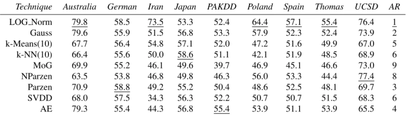
We next compare logistic regression using the normal process to a selection of one-class classifiers at an imbalance of 99:1. Optimised thresholds are calculated for all techniques used. The results of this comparison are displayed in Table 10 and are, in general, very similar to the results in Section 5.3. Logistic regression remains the best performing classifier. Further to the results of theHmeasure, in which logistic regression performs significantly better thank -NN and MOG, the performance of logistic regression with an optimised classification threshold is significantly better than a number of one-class classifiers (including SVDD, na¨ıve Parzen, mixture of Gaussians andk-NN). Of the one-class one-classifiers, based on average ranking, the Gaussian performs best. Based on the average ranking, it is worth noting that the harmonic mean performance of the SVDD classifier is somewhat worse compared to its corresponding Hmeasure performance. This difference highlights the sensitivity of selecting appropriate SVDD parameters at a specific classification threshold.
Table 10: Test set harmonic mean performance of logistic regression normal process (LOG Norm), and OCC process at a class imbalance ratio of 99:1. The best test set harmonic mean per data set is underlined. The average rank (AR) of the classifiers is also provided. Harmonic mean figures
should be multiplied by 10−2.
Technique Australia German Iran Japan PAKDD Poland Spain Thomas UCSD AR LOG Norm 79.8 58.5 73.5 53.3 52.4 64.4 57.1 55.4 76.4 1 Gauss 79.6 55.9 51.5 56.8 53.3 57.9 52.3 52.4 73.9 2 k-Means(10) 67.7 56.4 54.8 57.1 52.0 47.2 51.6 49.9 67.0 5 k-NN(10) 66.4 55.6 50.0 58.6 51.1 42.1 51.9 48.5 68.9 6 MoG 69.9 55.2 46.1 49.6 39.7 46.9 45.1 46.6 73.0 9 NParzen 63.5 53.8 46.8 49.8 46.3 56.0 53.3 44.4 77.4 8 Parzen 70.9 58.8 49.2 55.2 50.4 48.6 52.5 48.1 69.7 3 SVDD 68.0 57.5 34.3 56.3 52.2 50.7 50.7 51.5 68.3 6 AE 79.3 55.4 44.3 56.8 55.4 53.9 51.1 53.9 65.5 4 To summarise, selecting an appropriate threshold can substantially improve the performance of a two-class clas-sifier. Similarly, by optimising the threshold of a one-class classifier a representative proportion of the training data is accepted as target data. As the harmonic mean measures performance at a specific threshold it is important to select appropriate classifier parameters.
6. Conclusions
This article presented an extensive evaluation of approaches to solving the low-default portfolio problem when building credit scoring models. We believe that when both target and non-target data is available, the semi-supervised OCC techniques should not be expected to outperform the supervised two-class classification techniques. This is based on the fact that two-class classifiers use more information during training. Our findings also match Lee and Cho
(2007) who performed a modest comparison of one- and two- class classifiers for response modelling and found that with a response rate (the minority class) of 1% or lower one should apply OCC to the majority class.
Sampling is one of the simplest and most popular solutions to the class imbalance problem. Although oversam-pling improves the performance of some two-class classifier, it does not lead to an overall improvement of the best performing classifiers, i.e. the strong do not become stronger. In fact in our experiment the performance of the best performing two-class classifier, logistic regression, registered a small decline when oversampling was applied which matches the results of Bellotti and Crook (2009). Based on these findings, oversampling should not be employed with logistic regression as a suitable technique to address the LDP problem.
Adjusting the threshold yields a large improvement in performance. It is therefore advisable to optimise the clas-sification threshold before pursuing some of the more sophisticated methods associated with data sampling and cost sensitive learning. Although many studies discuss the importance of classification threshold selection (see Baesens et al., 2003), very few actually conduct any sort of assessment of the predictive performance of classifiers using an optimised classification threshold. Many studies sidestep the problem of choosing a specific classification threshold by using the AUC. However, as demonstrated by Hand (2009), it is“inappropriate”to compare classifiers using the AUC.
Using OCC, however, can allow financial institutions to reduce their dependency on expert human judgement during the construction of a LDP model. It also reduces the need to pool external data, combine different loan segments or expand the definition of a defaulter in order to boost the number of non-credit worthy applicants. Even though it cannot be unanimously proven that OCC is better than two-class classification at very low levels of defaulters, the performance of OCC merits consideration as a solution to the LDP problem.
It is important to note, furthermore, that the two-class classification methods are based on modelling both the distribution of past loan repayers and past defaulters. Whereas one-class classification methods are modelled solely on the distribution of past loan repayers. In situations ofpopulation drift, where the behaviour of defaulters changes over time due to unrecorded macro-economic factors or, indeed, personal reasons, then the performance of the two-class two-classifiers will deteriorate. This has been proven by Juszczaket al.(2008) in the field of fraud detection whose findings indicate that supervised classifiers, to some degree, overfit the current training data set such that when drift is introduced to the class distributions, the supervised classifiers deteriorate faster than the semi-supervised classifiers. This has serious implications for areas such as microcredit. Consider payday loans which are typically small, short duration (less than one month) with extremely high interest rates. It is necessary to construct scorecards that can respond in a timely fashion to shifts in economic and market behaviour, as well as to sudden changes in the borrower’s circumstances and behaviour (Thomas, 2009). Clearly one-class classification is suited to such tasks.
Future work should concentrate on situations for which OCC is well suited. OCC is best applied in situations with a heterogeneous non-target class where it can be difficult to model or obtain representative training examples. In retail loans the reasons for defaulting are typically unvarying across the portfolios (e.g. loss of income, loss of job, marriage breakdown, poor health). However for models which include economic and market conditions and can thus experience differing scenarios of an economic cycle, two-class classifiers may not be able to model all heterogeneous loan defaulters.
Future work could also look at more sophisticated OCC techniques that can utilise small amounts of non-target data. A more sophisticated form of oversampling, such as SMOTE (Chawlaet al., 2002), could also be examined. Another feature of oversampling to consider is the class distribution ratio. Khoshgoftaaret al.(2007) reported that an even distribution is not always optimal when dealing with data rarity. To ensure a more representative minority class, clusters could be identified in the minority class from which to sample the data.
Finally, the fact that OCC techniques did not yield significantly better performance should not exclude it as an ap-proach to the LDP problem. Thomas (2009) highlights the idea that a new methodology, using the same characteristics of the data as used by existing methods, producing a superior performance is questioned by many experts (see Hand, 2006). Indeed, Overstreetet al.(1992) observe that based on the flat maximum effect, the predictive performance of supposedly different classification techniques is almost indistinguishable as it is likely that most classification tech-niques will generate a model close to the best discrimination possible. Many other issues need to be considered when comparing the performance of a model, some of which have been outlined above and will be addressed in future work.
Acknowledgments
The authors would like to thank the Editor and two anonymous referees for their assistance in the preparation of this paper. In particular we would like to thank one of the referees for their informed response on theHmeasure.
References
Baesens, B., Gestel, T. V., Viaene, S., Stepanova, M., Suykens, J., and Vanthienen, J. (2003). Benchmarking state-of-the-art classification algorithms
for credit scoring.J Opl Res Soc,54, 627–635.
Baesens, B., Mues, C., Martens, D., and Vanthienen, J. (2009). 50 years of data mining and OR: upcoming trends and challenges.J Opl Res Soc,
(pp. S16–S23).
Basel Committee on Banking Supervision (BCBS) (2001, Revised Edition 2005).The Internal Ratings-Based Approach - Consultative Document.
Bank for Intl Settlements: Basel.
Basel Committee on Banking Supervision (BCBS) (2005, Comp v 2006). Intl Convergence of Capital Measurement and Capital Standards - A
Revised Framework. Basel II. Bank for Intl Settlements: Basel.
Bellotti, T., and Crook, J. (2009). Credit scoring with macroeconomic variables using survival analysis.J Opl Res Soc,60, 1699–1707.
Bishop, C. M. (1994). Novelty detection and neural network validation.IEE Proc-Vision, Image and Signal processing,141, 217–222.
Bishop, C. M. (1995).Neural Networks for Pattern Recognition. Oxford Uni Press, UK.
British Bankers Asc (BBA) (2004). Introductory Paper on Low Default Portfolios. http://www.isda.org/c_and_a/pdf/
ISDA-LIBA-BBALowDefaulPortfolioPaper-January2005.pdf. Accessed 25 June 2010.
Chandola, V., Banerjee, A., and Kumar, V. (2009). Anomaly detection: A survey.ACM Computing Surveys (CSUR),41, 15.
Chang, C.-C., and Lin, C.-J. (2001). LIBSVM: a library for support vector machines. Software available athttp://www.csie.ntu.edu.tw/
~cjlin/libsvm.
Chawla, N., Bowyer, K., Hall, L., and Kegelmeyer, W. (2002). SMOTE: synthetic minority over-sampling technique. J of AI Research,16,
321–357.
Chawla, N. V., Japkowicz, N., and Kotcz, A. (2004). Special issue on learning from imbalanced data sets.ACM SIGKDD Explorations Newsletter,
6, 1–6.
Chawla, S., Hand, D., and Dhar, V. (2010). Outlier detection special issue.Data Mining and Knowledge Discovery,20, 189–190.
Council of Mortgage Lenders (2009). CML reports decline in arrears and repossessions.http://www.cml.org.uk/cml/media/press/2680.
Accessed 12 August 2010.
Cover, T., and Hart, P. (1967). Nearest neighbor pattern classification.IEEE Transactions on Information Theory,13, 21–27.
Desai, V., Conway, D., Crook, J., and Overstreet, G. (1997). Credit-scoring models in the credit-union environment using neural networks and
genetic algorithms.IMA J of Management Math,8, 323.
Dionne, G., Art´ıs, M., and Guill´en, M. (1996). Count data models for a credit scoring system.J of Empirical Finance,3, 303–325.
Duda, R. O., and Hart, P. E. (1973).Pattern classification and scene analysis. Wiley, New York.
Duin, R., Juszczak, P., Paclik, P., Pekalska, E., de Ridder, D., Tax, D., and Verzakov, S. (2008).PRTOOLS (V4.1.4). A Matlab toolbox for pattern
recognition. Delft Uni of Tech, ICTG, NL.http://www.prtools.org.
Eisenbeis, R. (1977). Pitfalls in the application of discriminant analysis in business, finance, and economics.J of Finance,32, 875–900.
Forrest, A. (2005). Likelihood Approaches to Low Default Portfolios. Credit Research Center (CRC), University of Edinburgh.
Friedman, M. (1937). The use of ranks to avoid the assumption of normality implicit in the analysis of variance.J of the American Stat Asc, (pp.
675–701).
van Gestel, T., and Baesens, B. (2009).Credit Risk Management: Basic Concepts. Oxford University Press, USA.
Hand, D. (2009). Measuring classifier performance: a coherent alternative to the area under the ROC curve.Machine Learning,77, 103–123.
Hand, D., and Henley, W. (1993). Can reject inference ever work?IMA Journal of Management Mathematics,5, 45.
Hand, D., and Yu, K. (2001). Idiot’s Bayes: Not So Stupid after All?Intl Statistical Review/Revue Intle de Statistique,69, 385–398.
Hand, D. J. (2006). Classifier technology and the illusion of progress.Stat Science,21, 1–14.
Hand, D. J., and Zhou, F. (2009). Evaluating models for classifying customers in retail banking collections. J Opl Res Soc, Online,
doi:10.1057/jors.2009.129.
Hastie, T., Tibshirani, R., Friedman, J., and Franklin, J. (2005). The elements of statistical learning: data mining, inference and prediction. The
Mathematical Intelligencer,27, 83–85.
Hempstalk, K. (2009).Continuous Typist Verification using Machine Learning. Ph.D. thesis The University of Waikato, New Zealand.
Henley, W., and Hand, D. (1996). A k-nearest-neighbour classifier for assessing consumer credit risk.The Statistician,45, 77–95.
Hinton, G. (1989). Connectionist learning procedures.AI,40, 185–234.
Hoff, K. J., Tech, M., Lingner, T., Daniel, R., Morgenstern, B., and Meinicke, P. (2008). Gene prediction in metagenomic fragments: a large scale
machine learning approach.BMC bioinformatics,9, 217.
Hoffmann, F., Baesens, B., Mues, C., Van Gestel, T., and Vanthienen, J. (2007). Inferring descriptive and approximate fuzzy rules for credit scoring
using evolutionary algorithms.European Journal of Operational Research,177, 540–555.
Holm, S. (1979). A simple sequentially rejective multiple test procedure.Scandinavian J of Statistics,6, 65–70.
Hosmer, D., and Lemeshow, S. (2000).Applied logistic regression. Wiley-Interscience.
Ingolfsson, S., and Elvarsson, B. (2010). Cyclical adjustment of point-in-time PD.J Opl Res Soc,61, 374–380.
Japkowicz, N. (1999).Concept-learning in the absence of counter-examples: An Autoassociation-based approach to classification. Ph.D. thesis
Rutgers, The State University of New Jersey.
Juszczak, P., Adams, N., Hand, D., Whitrow, C., and Weston, D. (2008). Off-the-peg and bespoke classifiers for fraud detection.Computational