Using Natural Language as Knowledge Representation in an Intelligent Tutoring System

(1)

i

Using Natural Language as Knowledge Representation

in an Intelligent Tutoring System

By

Sung-Young Jung

Bachelor, Korea Advanced Institute of Science and Technology, 1994 Master, Korea Advanced Institute of Science and Technology, 1996

Master, University of Pittsburgh, 2008

Submitted to the Graduate Faculty of Intelligent Systems Program in partial fulfillment

of the requirements for the degree of Doctor of Philosophy

University of Pittsburgh

(2)

ii

UNIVERSITY OF PITTSBURGH

INTELLIGENT SYSTEMS PROGRAM

This dissertation was presented

by

Sung-Young Jung

It was defended on August 29, 2011 and approved by

Kurt VanLehn, Professor, School of Computing, Info. and Decision Systems Eng., Arizona State University Kevin D. Ashley, Professor, School of Law, University of Pittsburgh

Daqing He, Associate Professor, School of Information Sciences, University of Pittsburgh Dissertation Director: Alan Lesgold, Professor, School of Education, University of Pittsburgh

(3)

iii

Copyright © by

Sung-Young Jung

(4)

iv

Using Natural Language as Knowledge Representation

in an Intelligent Tutoring System

Sung-Young Jung, Ph.D. University of Pittsburgh, 2011.

Knowledge used in an intelligent tutoring system to teach students is usually acquired from authors who are experts in the domain. A problem is that they cannot directly add and update knowledge if they don’t learn formal language used in the system. Using natural language to represent knowledge can allow authors to update knowledge easily. This thesis presents a new approach to use unconstrained natural language as knowledge representation for a physics tutoring system so that non-programmers can add knowledge without learning a new knowledge representation. This approach allows domain experts to add not only problem statements, but also background knowledge such as commonsense and domain knowledge including principles in natural language. Rather than translating into a formal language, natural language representation is directly used in inference so that domain experts can understand the internal process, detect knowledge bugs, and revise the knowledgebase easily. In authoring task studies with the new system based on this approach, it was shown that the size of added knowledge was small enough for a domain expert to add, and converged to near zero as more problems were added in one mental model test. After entering the no-new-knowledge state in the test, 5 out of 13 problems (38 percent) were automatically solved by the system without adding new knowledge.

(5)

v

LIST OF FIGURES

Figure 1: The problem statement of the Skateboarder problem ... 3

Figure 2: Predicates defining a principle, Projection. ... 4

Figure 3: A statement of the Skateboarder problem represented in formal language ... 4

Figure 4: the generated equation for the skateboarder problem ... 5

Figure 5: (a) physics representation and (b) math of the skateboarder problem. ... 7

Figure 6: formal and natural language representations of the skateboarder problem. ... 9

Figure 7: the projection principle represented in formal language and natural language... 9

Figure 8: background knowledge translating the input sentences into physics representations. ... 11

Figure 9: The five types of knowledge represented in natural language, and their data flow during problem solving... 12

Figure 10: the system architecture of Natural-K ... 13

Figure 11: the basic form of an implication rule ... 14

Figure 12: examples of default rules ... 14

Figure 13: An example for positive and negative facts, and positive, negative, and unknown conditions 15 Figure 14: an example of negation rule (A does not imply B). ... 15

Figure 15: the basic form of a principle ... 16

Figure 16: the basic from of a truth rule ... 16

Figure 17: examples of truth rule ... 17

Figure 18: a qualitative question and a truth rule to check the validity ... 17

Figure 19: examples of truth rule for logic and math ... 18

Figure 20: an example sentence and a truth rule for math to calculate the actual direction (35+90 degrees) ... 18

Figure 21: generalizing by making shorter ... 19

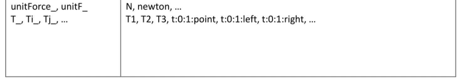
Figure 22: predefined semantically binding variables ... 20

Figure 23: example rules using semantically binding phrase variables ... 20

Figure 24: a fact with a time point ... 21

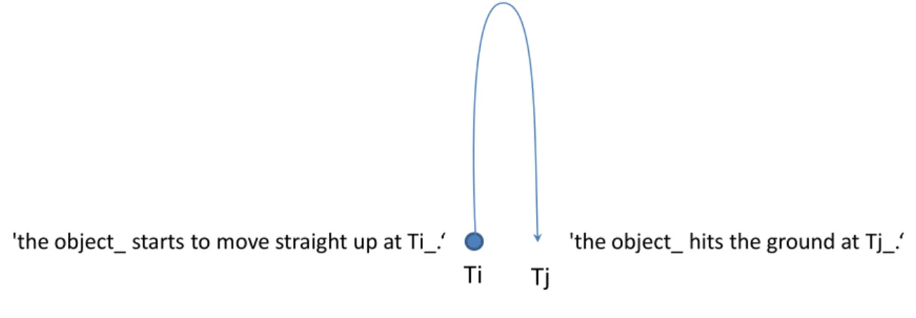
Figure 25: Problem statement of throwing upward ... 21

Figure 26: creating a new time point ... 22

Figure 27: The form of time index and examples. ... 22

Figure 28: creating a new time interval ... 23

Figure 29: generated facts with a time index assigned ... 23

Figure 30: an example with two time intervals ... 23

Figure 31: Time index and time value assignment ... 24

Figure 32: The generated facts with a final time value assigned. ... 24

Figure 33: Time index and time value assignment when two time intervals are given. ... 24

Figure 34: a sentence with a conjunctive time phrase, and a rule to recognize it ... 25

Figure 35: an example of to-infinite time phrase, and a rule to interpret ... 25

Figure 36: an example of adjective time phrase (initial~, final~, whole~, total~), and rules to interpret .. 26

(9)

ix

Figure 38: a mental model for projectile movement represented in formal language in Pyrenees ... 27

Figure 39: the basic mental model for throwing upward ... 28

Figure 40: a rule for starting movement ... 28

Figure 41: a rule for movement at the interval and the final event ... 29

Figure 42: a rule for the event returning to the initial level of height ... 29

Figure 43: generated facts with a time index ... 29

Figure 44: generate facts with a time point ... 29

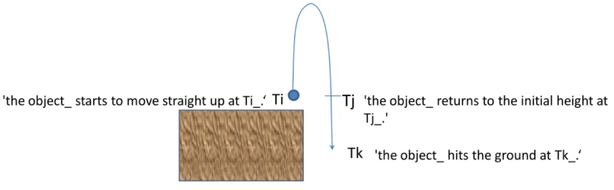
Figure 45: throwing upward on a high place ... 30

Figure 46: the background rule for throwing upward in a high place. ... 30

Figure 47: a logic rule to generate a mid time point. ... 30

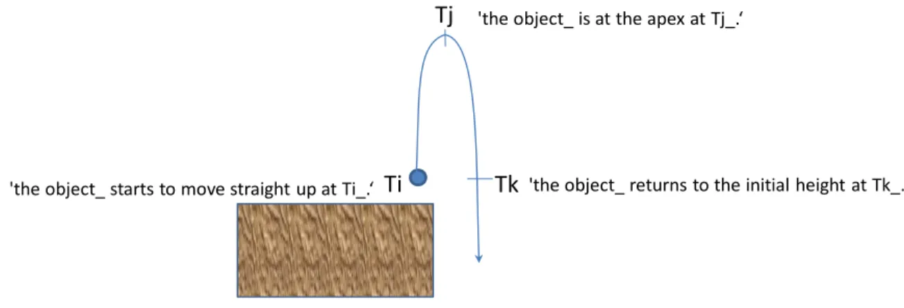
Figure 48: throwing upward and reaching the apex ... 31

Figure 49: the mental model extension rule for reaching the apex ... 31

Figure 50: A ring thrown upward from the roof of a building ... 31

Figure 51: a background rule for the apex ... 31

Figure 52: two principles for the throwing-upward mental model. (a) Initial and final velocities (b) displacement and initial velocity ... 32

Figure 53: generated facts by the basic mental model ... 32

Figure 54: generated facts by the extended mental model ... 33

Figure 55: generated facts by the extended mental model for reaching the apex ... 33

Figure 56: background rules for the last two questions ... 33

Figure 57: the two questioned translated in physics representation ... 33

Figure 58: the produced facts with time index attached ... 34

Figure 59: generated facts at the end of the inference stage ... 35

Figure 60: generated equations ... 35

Figure 61: the output of the equation solver ... 35

Figure 62: The final answers generated ... 35

Figure 63: an example of default knowledge that can generate different results depending on application order ... 38

Figure 64: over-generation example (an input sentence, two rules, and the two facts generated)... 38

Figure 65: Subsumption relations drawn as directed graph ... 39

Figure 66: an example of inference failure due to a time phrase ... 39

Figure 67: a background rule inferring projectile movement ... 40

Figure 68: an example of syntactic ambiguity (prepositional attachment). (a) an input sentence (b) two interpretations in formal language. ... 42

Figure 69: Ambiguity resolution in the natural language representation (a) the input sentence followed by another sentence (b) a background rule to infer that the airplane was on the hill (c) another example of the input sentence followed by another sentence (d) a background rule to infer that the man was on the hill. ... 42

Figure 70: Previous approaches to transform natural language to formal language ... 43

Figure 71: knowledge in unconstrained natural language ... 44

(10)

x

Figure 73: A chart containing all parse trees generated is used as internal representation of a sentence.

... 46

Figure 74: Syntactic normalization of a passive form ... 47

Figure 75: a relative clause and its variation ... 48

Figure 76: sentence normalization for relative clause ... 48

Figure 77: Sentence normalization for conjunctive phrase. ... 48

Figure 78: A normalization link in a least common ancestor (LCA)=’pushed’. (a) The LCA of ‘pushed’ and ‘man’ is ‘pushed’. So activate the link (b) the LCA of ‘pushed’ and ‘man’ is ‘was’. So inactivate the link.. 49

Figure 79: a background rule designating a physics object. ... 49

Figure 80: (a) an example of a pronoun in which recency heuristics fails, (b) a background rule required to resolve the pronoun ‘it’ ... 50

Figure 81: an example of background rule with a pronoun ‘it’ ... 50

Figure 82: the number of rules added for each physics problem in Pyrenees ... 53

Figure 83: the number of rules added for each physics problem in Young&Freeman’s Textbook ... 54

Figure 84: the number of background rules added for each physics problem in Throw-upward mental model ... 55

Figure 85: reasons of the added rules for the problems in the throw-upward mental model (a) for a mental model (b) for time phrases (c) for paraphrases (d) for questions. ... 56

Figure 86: an example of rewording. (a) An original problem statement (b) a reworded statement (c) the number of edits ((w) is a deletion, (w1->w2) is a modification, and the others are addition) ... 58

Figure 87: The min-edit distance after the tenth problem (total 13 problems). ... 58

Figure 88: the number of mental models in each of three chapters in Young and Freedman’s textbook. 59 Figure 89: An example of (a) a problem statement, (b) a reworded statement, and (c) added rules by the subject4 ... 61

Figure 90: The min-edit distance for each of the recruited subjects ... 62

Figure 91: The number of rules added by each subject ... 63

Figure 92: The min-edit distance, time spent, and the number of trials in average across the subjects. .. 63

Figure 93: The number of rules added, time spent, and the number of trials in average across subjects 64 Figure 94: Question1 ... 64

Figure 95: Question2 ... 65

Figure 96: Question3 ... 65

Figure 97: The main two factors determining convergence of the size of required knowledge. ... 66

Figure 98: comparison of three types of tutoring systems and the size of knowledge to add. ... 67

Figure 99: A new dimension of ITS types ... 68

Figure 100: Examples to deal with ambiguity: (a) an input sentence (b) an over-generated case due to the prepositional attachment (c) removing the over-generated output by rewriting the rule to be more specific (d) removing the over-generated output by copy-and-pasting the input sentence to the rule. .. 70

Figure 101: Inference log of the case1 of Figure 100 ... 71

Figure 102: over-generation example ... 71

Figure 103: the problem statement of Balloon Problem ... 72

Figure 104: An example generating hits ... 73

(11)

xi

Figure 106: inference steps of the Balloon problem. ... 73

Figure 107: background knowledge for the balloon example ... 74

Figure 108: An example of an ITS helping a student how to understand the Balloon problem (Figure 103). ... 75

Figure 109: the process of student’s adding the skateboarder problem to the system. ... 76

Figure 110: An example of an article (a) in a law book (b) in a form of rule ... 76

Figure 111: An example of a bill of indictment ... 77

Figure 112: an example of background knowledge to interpret the bill of indictment ... 77

Figure 113: a generated fact ... 77

Figure 114: The final sentence generated ... 77

Figure 115: examples of paraphrase ... 80 Figure 116: semantically binding variables with an underbar (upper) and without an underbar (lower) . 84

(12)

xii

PREFACE

This dissertation was possible by the full support of my advisor Dr. Kurt VanLehn who inspired me to go deep into the core problem of artificial intelligence that was believed to be infeasible for a long time. It required big ambition, courage, and adventurous spirit to break through the barriers in the land where no one has ever set foot. During this research, I got convinced that artificial intelligence was around the corner. I hope that this dissertation helps readers to share my experiences and to have courage to go for the dream. I also want to thank Dr. Alan Lesgold, Dr. Kevin Ashley, and Dr. Daqing He for giving me invaluable comments and advice.

(13)

1

1.0 INTRODUCTION

An Intelligent Tutoring System (ITS) can teach students to learn and acquire domain knowledge provided by the system, and the system needs to acquire such knowledge from authors who are domain experts (Murray, 2003). Although one might be able to team a domain expert with a programmer for the initial development of such a system, that approach is not sustainable. For example, high school teachers who don’t know computer programming and a formal language may want to add new domain problems to use in their class. Moreover, different teachers have different directions and preferences on class materials, and would like an ITS to which they can add their own domain problems for their class.

During the authoring process, authors should be able to follow each step of the problem solving, detect errors, and fix them by adding and updating knowledge. They may not be able to do such tasks if the knowledge is represented in formal language. Although it is possible that the system generates natural language explanations of its reasoning from the formal language, domain experts still cannot edit the knowledge directly. This suggests developing a system using natural language to represent knowledge so that non-programmers can easily develop and maintain ITS knowledge.

The thesis addresses mainly a goal to find a way to represent required background knowledge in natural language so that the system can understand a problem statement and solve it like a student can read and solve it. The other goal is to find a way to represent generalized knowledge in natural language so that the size of knowledge which domain experts have to add decreases as more problems are added, and converges to near zero. All the other knowledge that the ITS needs, e.g., in order to solve problems and coach students during problem solving, is built into the ITS in a domain-general fashion, so that authors need never examine it nor debug it. In short, the proposed system is intended primarily for use by domain experts to add domain problems to an existing ITS. It can also be used to add domain problems to an initially empty ITS, but that usage is secondary.

Some studies of applying natural language understanding to tutoring systems were performed before. Novak developed a physics problem solving system, ISAAC, that reads a problem statement written in natural language and solved the given problem (Novak Jr., 1977). ISAAC received natural language input and transformed it into semantic frames which were a kind of formal representation. A physics problem solver, MECHO (Bundy, Byrd, Luger, Mellish, & Palmer, 1979), also transformed a problem statement into formal language.

These and other studies evaluated the potential of the idea adopting natural language as input form of knowledge for problem statements. However, the advantage was limited because background knowledge such as commonsense knowledge had to be encoded inside program routines. Only computer programmers were able to update such knowledge. So, adding a new domain problem was limited to cases where all required background knowledge was already encoded in the systems. If a domain problem failed to be translated properly or the background knowledge was incomplete, then the author had no easy way to fix or even understand the flaw. This suggests that authors must be able to read and edit the background knowledge as well as the problem statements.

(14)

2

Acquiring knowledge from natural language is an old idea in the natural language processing area. A common approach in this idea was to transform natural language into formal representations such as logic forms (Jurafsky & Martin, 2000)(Brachman & Levesque, 2004) or semantic networks (Sowa, 1990)(Shastri, 1990). Using precise formal representations after transformation, the systems performed inference to accomplish a goal. In modern work on knowledge capture and knowledge acquisition, formal language was commonly used to represent knowledge in systems such as KANTOO(Nyberg, Mitamura, & Betteridge, 2005), KAT (Moldovan, Girju, & Rus, 2000.), and WordNet2 (Harabagiu, Miller, & Moldovan, 1999). In other systems, such as AURA (Chaudhri, John, Mishra, Pacheco, Porter, & Spaulding, 2007) and SHAKEN (Clark, et al., 2001), domain experts transformed contents of science textbook to graphical notations which is another form of formal language. The main problem of this approach was that still only knowledge engineers and programmers could update the formal language when update is needed, and knowledge required for transformation (such as templates) was implicitly encoded in program code, thus also only programmers could update it.

Another direction comparable to this thesis is to use natural language to represent logic. There have been several such studies. For instance, Natural Logic is an approach to recognize textual entailment (MacCartney & Manning, 2008). Controlled Natural Language restricts natural language syntax to use English as formal language (Fuchs, Kaljurand, & Kuhn, 2008). Logic-oriented studies mainly focus on obtaining sound logical inferences rather than expediting knowledge acquisition. A problem in this approach rises when some knowledge cannot be represented in given constraints. Then again, only programmers can change the constraints.

A common issue in the previous studies was that using natural language in knowledge representation requires a proper way to deal with commonsense knowledge. One of the problems known in this approach is that there can be million different natural language expressions for the same element of underlying knowledge and there is no easy way to recognize them. This is called the paraphrasing problem. Textual entailment is an area dedicated to find a way for this problem. For example, “the force applied to the object” textually entails “the force exerted to the object”. Using enough background knowledge has been recognized as one of the most important factors in the textual entailment (Iftene, 2009).

As the needs for commonsense knowledge increased in many AI systems, attempts to build commonsense knowledge base started, such as Opencyc (OpenCyc Tutorial), Learner (Chklovski, 2003), OpenMind (Speer, 2007), MindNet (Dolan & Richardson, 1996), and TextNet (Harabagiu & Moldovan, 1994). They try to build a universal commonsense knowledgebase represented in formal language. However, it is unlikely that the complete set of universal commonsense knowledge can be built soon. Such resources were not used in this thesis because what we need is a small set of knowledge required to solve a given domain problem rather than the complete set of universal knowledge.

A dilemma of knowledge representation in natural language was that commonsense knowledge was needed but it was not available. A basic approach for this issue is that commonsense knowledge can be acquired in natural language from authors too. Because an ITS is task specific, it is hypothesized that the amount of knowledge to add per a problem is feasibly small for an author to add in an ITS. The

(15)

3

validity of this hypothesis will be tested by authoring physics problems from textbooks in studies (section 12.2).

This thesis presents a way to allow authors to add not only problem statements, but also background knowledge including commonsense and domain knowledge. The main approach is to use unconstrained natural language to represent knowledge so that authors can understand knowledge, add knowledge, detect bugs, and fix them easily.

2.0 THE PREVIOUS ITS: PYRENEES

The previous ITS, Pyrenees is presented here shortly to demonstrate the problems and difficulties clearly. The new system Natural-K will be presented later, and it was driven from Pyrenees to overcome the difficulties.

2.1. FORMAL LANGUAGE REPRESENTATION OF PYRENEES

Pyrenees is a model-tracing tutoring system for equation-based problems. It teaches students both the principles themselves and how to apply them to solve a problem efficiently. All of its pedagogical knowledge is hardwired into it, so the author need only provide the domain knowledge. Although it has been used with several task domains (including thermodynamics, statistics and microeconomics), introductory mechanics is the target domain. Domain knowledge in Pyrenees includes a set of problems, a set of principles and ontology. Problems are solved by finding a relevant set of equations then solving them algebraically. Each equation should be an instance of a general principle. For instance, consider a problem such as the following (Figure 1):

Figure 1: The problem statement of the Skateboarder problem The set of relevant equations is:

 V= 1.3 m/s   = 143 degrees  Vy = V * sin ()

where V is the magnitude of velocity of the skateboarder,  is the direction of movement of the skateboarder, and Vy is the y component of the velocity. The first two equations are givens, and the last equation is an equation of a general principle. In the existing system, each variable is internally represented in first order logic as follows:

 V : var(at(mag(velocity(skateboarder)), tpt(1)))   : var(at(dir(velocity(skateboarder)), tpt(1)))

 Vy: var(at(compo(velocity(skateboarder), axis(y, dnum(0, deg))), tpt(1))) Skateboarder Problem:

‘A skateboarder rolls at 1.3 m/s up an inclined plane angled at 143 degrees. What is her vertical velocity?’

(16)

4

This says, for instance, that Vy is a variable (var) denoting the value at time point 1 (tpt(1)) of the component (compo) along the y-axis of an unrotated coordinate system (axis(y,dnum(0,deg))) of the velocity of the skateboarder.

There are three domain knowledge bases: ontology, principles, and problems. The ontology

describes the domain objects, properties and relationships, as well as how to translate each formal term into English. For instance, the ontology would indicate that skateboarder is an object, that at(mag(velocity(skateboarder)), tpt(1)) is a quantitative property, and that

var(at(mag(velocity(skateboarder)), tpt(1))) is an algebraic variable for that quantitative property. The second knowledge base is a set of principles. Principles are represented in formal language. Figure 2 shows a principle written in the Prolog code used by Pyrenees. The name of the principle is

Projection. This principle receives three arguments, Vector, T and Ax, and returns a problem-specific equation. For instance, if it receives Vector=velocity(skateboarder), T=tpt(1), and Ax=axis(y, dnum(0, deg)), then it returns the equation in Figure 4.

pa_equation (along(projection(offaxis, Vector, T), Ax), V_x=V*Trig) :- V_x = var(at(compo(Vector, Ax), T)),

V = var(at(mag(Vector), T)), V_dir = var(at(dir(Vector), T)),

offaxis_projection_trig(V_dir, Ax, Trig).

offaxis_projection_trig(V_dir, axis(x, Rot), cos(V_dir-Rot)). offaxis_projection_trig(V_dir, axis(y, Rot), sin(V_dir-Rot)). Figure 2: Predicates defining a principle, Projection.

The third knowledge base is a set of problems. Like the principles, these are expressed in terms of the formal language. Figure 3 illustrates the skateboarder problem represented in formal language. The known quantities are given inside known(…) term, and the sought quantity is given in sought(…) term. p_definition(skateboarder,

[time_points([1]),

physical_object(skateboarder),

known(var(at(mag(velocity(skateboarder)), tpt(1))), dnum(1.3, m/s)), known(var(at(dir(velocity(skateboarder)), tpt(1))), dnum(143, deg)), coordinate_system_given(dnum(0, deg)),

sought(var(at(compo(velocity(skateboarder), axis(y, dnum(0, deg))), tpt(1))), dnum(0.78, m/s)) ]).

Figure 3: A statement of the Skateboarder problem represented in formal language

Pyrenees solves problems via a version of backward chaining called the Target Variable Strategy (Chi & VanLehn, 2007)(VanLehn, et al., 2004)(Chi & VanLehn, 2008). The basic idea is simple: Given a sought quantity, generate an equation that applies to this problem and contains the sought quantity. If the equation has any quantities in it that are neither known nor previously sought, then treat them as

(17)

5

sought and recur. When the Target Variable Strategy stops, it has generated a set of equations that are guaranteed to be solvable.

In the case of the problem above, the Pyrenees would start with the variable

var(at(compo(velocity(skateboarder), axis(y, dnum(0, deg))), tpt(1))) as the sought quantity. It then checks all its principles, and finds that the principle in Figure 2 has a term in its equation that unifies with the variable. This unification binds Vector to velocity(skateboarder), T to tpt(1), and Ax to axis(y, dnum(0, deg)) and creates the equation as Figure 4.

var(at(compo(velocity(skateboarder), axis(y, dnum(0, deg))), tpt(1))) =

var(at(mag(velocity(skateboarder)), tpt(1))) * sin(var(at(dir(velocity(skateboarder)), tpt(1)))-0). Figure 4: the generated equation for the skateboarder problem

Pyrenees notes that the equation has two quantities in it. The first is

var(at(mag(velocity(skateboarder)), tpt(1))). It checks the problem statement, and discovers that this quantity is known, so it does not need to recursively seek a value for it. It now consider the second quantity in the equation, var(at(dir(velocity(skateboarder)), tpt(1))). That too is known, so Pyrenees is done with this problem, having “written” just one equation.

The take-home message of this section is that even though the skateboarder problem (Figure 1) is extremely simple, the formality of the knowledge used to represent and solve it would be a serious impediment to an author who has neither the time, skills, or inclination to master it.

2.2. DIFFICULTIES IN AUTHORING IN FORMAL LANGUAGE

The first obvious difficulty in authoring Pyrenees is in understandability. Let’s take a look at the sought quantity again.

var(at(compo(velocity(skateboarder), axis(y, dnum(0, deg))), tpt(1)))

It is unrealistic to expect that domain experts can easily understand and write such quantities represented in formal language. So, they cannot participate in authoring using this representation. Also, it is difficult to read even for a knowledge engineer. The second difficulty in authoring is in parenthesis. In a case where a knowledge engineer writes the quantity in formal language, the mis-matching parenthesis is a frequent source of mistakes and errors. Syntax directed editors will balance the parentheses, but they may not know the argument structure of the knowledge representation, which makes mismatching parentheses hard to detect. The first line below is wrong and the second is correct, but they are hard to tell apart:

var(at(compo(velocity(skateboarder), axis(y, dnum(0, deg)), tpt(1)))) var(at(compo(velocity(skateboarder), axis(y, dnum(0, deg))), tpt(1)))

Humans can understand and communicate without parenthesis using natural language. A natural language sentence looks simpler and easier, and the chance of writing an error is much smaller without parenthesis. Let’s look at the variable represented in natural language and compare it to the above formal version to see how easily authors can understand.

(18)

6 “The vertical velocity of the skateboarder at T1”

The third difficulty is in the strict argument ordering of formal language. Each of arguments should be given in predetermined order. An author should remember the order and the required set of arguments for each quantity. Following are simplified examples for force. There can be different argument orders and all of them except one are errors to the system. The author should remember the right order of arguments for each quantity, and it is a big burden.

force(agent, object, applied) : correct force(object, agent, applied) : incorrect force(agent, applied, object) : incorrect force(object, applied, agent) : incorrect

In the case of natural language representation, syntactic constraints using prepositions have a role in determining arguments. It is naturally understood by authors, and the system also can accept them without a big difficulty.

“The applied force exerted to the object by the agent” “The force applied to the object by the agent”

“The force applied by the agent to object”

It is possible to display quantities in natural language from the formal language using a generation module, but domain experts still cannot edit them directly.

In previous approaches, it was common to use natural language for authors and transform to formal language for a system. However, transforming between natural and formal languages had many problems such as lack of flexibility, extensibility, and difficulty in managing commonsense knowledge, etc. Basically, the difficulties were from the situation that programmers had to change transformation modules containing transformation knowledge whenever a new pattern of knowledge should be added. The idea presented in this thesis is to use natural language directly without transforming to formal language to avoid such difficulties.

Natural language representation is more easily learned than formal language, which lowers the barriers for instructors and even students to add knowledge to the ITS. Besides understandability and learnability, natural language allows the problem solver’s reasoning and its knowledge to be understood more easily. This is important when the user must trust the system. Generating natural language explanation from knowledgebase in formal language is a challenging problem (Swartout, Paris, & Moore, 1991 ) (Eugenio, Fossati, Yu, Haller, & Glass, 2005), but using natural language as knowledge representation enables explanation generation without difficulty. This thesis presents a new approach using natural language as knowledge representation avoiding the difficulties in using formal language: understandability, learnability, and explanation generation.

(19)

7

3.0. TYPES OF KNOWLEDGE IN THE THREE LEVELS IN PHYSICS

Three levels of knowledge representation are involved in physics problem solving, i.e. naïve representation, physics representation, and math representation (Larkin J. , 1983). As an example, let’s take a look at the skateboarder problem again (Figure 1). The problem statement is written in unconstrained natural language which does not use the academic language of physics. This representation of a problem is called the naïve representation.

To solve this physics problem, the naïve representation should be translated into a well-defined representation that clarifies the given physics situation precisely. The concepts in physics implicitly given in naïve representation (e.g. velocity, acceleration, force, etc.) should be mentioned explicitly. This articulation of the problem in the academic language of physics is called its physics representation. In Figure 5-(a), the magnitude, direction, and y-component of the velocity were listed.

Lastly, the math representation restates the problem in mathematical form. By applying physics principles, one can create a solvable set of equations that represents the problem. More specifically, the equations can be solved algebraically yielding values for all the variables, and every equation is either an assignment of variable’s value that is given in the problem statement, or the application of a physics principle that is justified by the problem statement. For instance, Figure 5-(b) shows the final representation of the skateboarder problem in its math representation.

(a) ‘The magnitude of the velocity of the skateboarder is 1.3m/s.’ ‘The direction of the velocity of the skateboarder is 143 degrees.’ ‘What is the y-component of the velocity of the skateboarder? ' (b) y=mag*sin(theta) , % projection principle

mag=1.3 m/s, theta=143 degrees, y=?

Figure 5: (a) physics representation and (b) math of the skateboarder problem.

Given that there are 3 representations, one would expect two types of knowledge for converting from naïve to physics representation, and physics to math representation. The first mapping, from the naïve (i.e. the input problem statement) to the physics representation, is driven by considerable informal background knowledge including commonsense. For example, the naïve representation “a skateboarder rolls at 1.3 m/s” implies that the skateboarder is a physical object, and it has a non-zero velocity of 1.3 m/s. Although this type of knowledge is sometimes called description phrase knowledge

(Larkin J. , 1983)(Hestenes, 1987), we prefer the simpler phrase background knowledge.

The second mapping, from the physics to the math representation, is driven by well-defined principle schemas. Each principle has conditions designating when to trigger. For example, this projection principle can be triggered when a physics object has a vector property (e.g., velocity) that is not aligned with an axis. This set of conditions plus other details are called a principle schema. Such schemas convert physics representations into math representations.

Some previous work, such as Fermi (Larkin J. H., 1998), Newton (De Kleer, 1975), Cascade (VanLehn, 1999), and AURA (David Gunning, 2010), have used formal representations exclusively. Input problems

(20)

8

were manually translated into formal language versions of a naïve representation. Thus, a partial formalization of “A skateboarder rolls up an inclined plane” would be physical_object(skateboarder), surface(plane), supported_by(skateboarder, plane), etc. The physics representation, math representation, background knowledge and principles schemas were all written in formal language.

Other previous works adopted a method to transform natural language into formal representations (Mecho (Bundy, Byrd, Luger, Mellish, & Palmer, 1979), ISAAC (Novak Jr., 1977), and pSAT (Ritter, 1998)(Ritter, Anderson, Cytrynowicz, & Medvedeva, 1998)). Their systems were designed to translate naïve representation in natural language into physics representation in formal language. In this approach, background knowledge included both domain-specific knowledge (e.g., an inclined plane is a surface) and natural language processing knowledge. This rather large, diverse knowledgebase was encoded in program code, and only the system developers were able to change it. So, they still had the same problem that only the system developers can change background knowledge and the other formal representations.

The proposed approach in this thesis is to represent both types of knowledge (background knowledge and principle schemas) in natural language, and to use natural language for the naïve and the physics representations. The math representation of physics problems will continue to be written in mathematical notation. In other words, because the naïve representation, background knowledge, physics representation, and principle schema are all represented in natural language, everything an author sees from the problem statement onward is in natural language until the very end, when the mathematical representation is generated by instantiation of generic equations that are part of the principle schemas. Because authors are assumed to already know math as well as English, they don’t need to learn new languages or new representations in order to work with the system.

4.0. REPRESENTING KNOWLEDGE IN NATURAL LANGUAGE

The problem statement needs to be interpreted so that it can trigger relevant principles. For the principles to be triggered, the problem must be described in terms of proper scientific concepts such as forces, accelerations and velocities. Let us define the physics representation more precisely to refer to the representation that directly matches the principle schemas. Thus, the physics representation of a problem must use proper scientific concepts such as forces, etc. In theory, the physics representation could use complex syntax (e.g., relative clauses), pronouns and other constructs of natural language. As long as a sentence can match rules triggering target principles, the system doesn’t care about the form of sentences. In this way the system allows authors to write the physics representation in free natural language. However, authors should write physics representations so that they can trigger relevant principles with limited matching conditions, so authors will tend to employ a fairly limited range of linguistic constructs for the physics representations

As an example, Figure 6 shows both a formal language and the corresponding natural language version of the physics representation of the skateboarder problem. It seems plausible that an author who is trying to debug the translation of a problem could more easily understand physics representation written in natural language (Figure 6-(b)) rather than formal language (Figure 6-(a)).

(21)

9 (a) Formal

language

known(at(mag(velocity(skateboarder)), tpt(1)), dnum(1.3, m/s)). known(at(dir(velocity(skateboarder)), tpt(1)), dnum(143, degree)). sought(at(comp(velocity(skateboarder), y), tpt(1))).

(b) Natural language

‘The magnitude of the velocity of the skateboarder is 1.3m/s at T1.’ ‘The direction of the velocity of the skateboarder is 143 degrees at T1.’ ‘What is the y-component of the velocity of the skateboarder at T1? ' Figure 6: formal and natural language representations of the skateboarder problem.

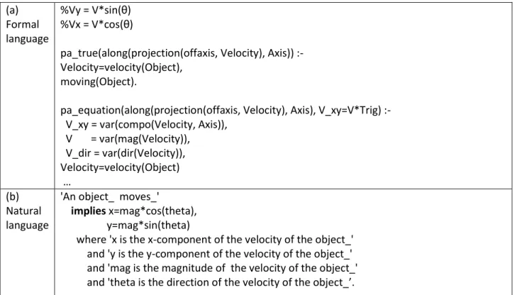
Although a principle includes a set of equations which should be instantiated when some conditions are satisfied, the rest of the principle can be represented in natural language. For example, Figure 7-(b) shows the projection principle in natural language. The principle has a condition checking whether the object is a moving object (i.e 'An object_ moves_'), and it corresponds to the principle schema. Notice that it is also represented in natural language here.

Definitions of variables used in a principle are represented in natural language too here. For example, the sentence “mag is the magnitude of the velocity of the object_” provides the definition of the variable mag in natural language. Thus, the definitions of the variables can be written by an author when he adds a principle. The system just finds matches from the known facts in the current context (Figure 6-(b)) to the definitions of variables in a principle (Figure 7-(b)) when triggering. In this way, everything except equations is defined in natural language.

(a) Formal language %Vy = V*sin(θ) %Vx = V*cos(θ)

pa_true(along(projection(offaxis, Velocity), Axis)) :- Velocity=velocity(Object),

moving(Object).

pa_equation(along(projection(offaxis, Velocity), Axis), V_xy=V*Trig) :- V_xy = var(compo(Velocity, Axis)),

V = var(mag(Velocity)), V_dir = var(dir(Velocity)), Velocity=velocity(Object) … (b) Natural language

'An object_ moves_'

implies x=mag*cos(theta), y=mag*sin(theta)

where 'x is the x-component of the velocity of the object_' and 'y is the y-component of the velocity of the object_' and 'mag is the magnitude of the velocity of the object_' and 'theta is the direction of the velocity of the object_’. Figure 7: the projection principle represented in formal language and natural language.

Physicists would immediately understand the principle schema expressed as Figure 7-(b), could confirm that it is correct, and could write other ones like it. On the other hand, they would require some training in order to understand the formal version of the projection principle shown in Figure 7-(a).

(22)

10

Even with training, because the formal language will always be relatively less familiar than the natural language, physicist might overlook minor errors such as misordering of arguments. This formal version of the principle was from a previous system written in Prolog, so physicists trying to use it would have to learn the computer language, Prolog in this case. We hypothesize that physics instructors would find it easier to write, check and debug the natural language versions.

These two figures represent the basic hypothesis. Although the domain mandates that the conceptual content be translated from naïve to physics to math concepts, it is much easier for authors to understand this translation if the content is written in natural language rather than a formal language.

4.1. REPRESENTING BACKGROUND KNOWLEDGE

The preceding section may suggest that in order to add a new problem to the tutoring system, the author could write a naïve representation to be read by students, and a physics representation in natural language to be read by the tutoring system. The physics schemas in the tutoring system would then translate the given physics representation into a math representation. If that translation failed, then the author could debug the newly written physics representation and/or the principle schemas since they are all written in natural language.

While feasible, the approach just sketched is far from optimal. Many researchers have noted learners make most of their mistakes when translating the naïve representation to the physics representation. For instance, learners often fail to notice when forces, accelerations, velocities, displacements and other physics entities are present. Indeed, the background knowledge is often considered the conceptual core of physics because the principle schemas are important, but not difficult to learn. Thus, the tutoring system needs to tutor the students as they apply background knowledge. This means that the tutoring system needs to have a representation of such knowledge. Of course, some of the background knowledge is familiar (e.g., a skateboarder is a physical object) so it doesn’t need tutoring.

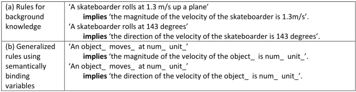
This motivated developing an intelligent system that can automatically generate physics representations from a naïve, natural language problem statement. In order to do so, the system should have background knowledge connecting the problem statement (naïve representation) to the physics representation. This knowledge includes the description phrase knowledge, and it can include linguistic knowledge, commonsense knowledge, and domain knowledge from physics. The idea proposed here is to represent background knowledge in natural language as inference rules, and to let authors add them.

(23)

11 (a) Rules for

background knowledge

‘A skateboarder rolls at 1.3 m/s up a plane’

implies ‘the magnitude of the velocity of the skateboarder is 1.3m/s’. ‘A skateboarder rolls at 143 degrees’

implies ‘the direction of the velocity of the skateboarder is 143 degrees’. (b) Generalized

rules using semantically binding variables

‘An object_ moves_ at num_ unit_’

implies ‘the magnitude of the velocity of the object_ is num_ unit_’. ‘An object_ moves_ at num_ unit_’

implies ‘the direction of the velocity of the object_ is num_ unit_’. Figure 8: background knowledge translating the input sentences into physics representations.

The background knowledge represented in natural language has a form of a rule with conditions and actions (Figure 8-(a)). The action produces a fact in physics representation. The condition matches the naïve representation and perhaps also some previously produced physics representation. Basically if one of the parse trees of the condition is a subtree of that of the input sentence, they can match (the matching method will be explained in details in chapter 11.0). These rules run in a forward chaining manner, like a production system, until they reach quiescence.

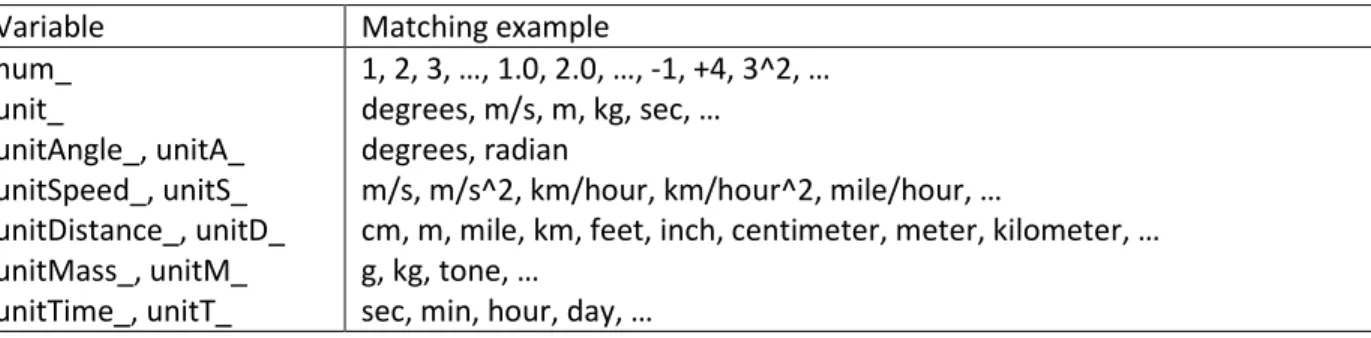
Introducing semantically binding variables (e.g. object_, moves_, num_, and unit_) can generalize the rule to be applied to broader cases (Figure 8-(b)). For example, object_ can match all nouns whose semantic class is ‘object’ such as ‘skateboarder’, ‘car’, etc. It is possible to develop a system to automatically generalize the set of rules added by authors. However the generalization module was not implemented because authors can directly write the generalized rules in natural language.

It is expected that the number of rules to be added decrease as more problems are added, and eventually converge to near zero per problem. Ideally, in order to add a new problem to the tutoring system, the author types in the naive representation to be read by the student, presses the “submit” button, checks that the physics representation and the math representation are what the author intended, and checks the final answer that the system generates. If any of the checks fail, then the author can try rewording the naïve representation (the problem statement). If rewording always succeeds, then the author never needs to examine the background knowledge, physics representation, etc. in detail in order to find a bug or missing knowledge. We call this happy state of affairs the no-new-knowledge state of the system. A question in this approach is about how many rules need to be added to the system in order to achieve the no-new-knowledge-state.

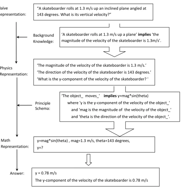
Figure 9 shows the overall flow of knowledge in the system. The input physics statement in naïve representation is translated to the physics representation using the background knowledge. The physics knowledge is translated to the math representation using the principle schema. The generated equations are solved, and the final answer is displayed. All types of knowledge are represented in natural language except the math equations at the end. As shown in the figure, every step of the process and inference can be understood easily by non-programmers. Thus this approach makes the system transparent to non-programmers enabling them to join the authoring task, and the intermediate inference results can be used to generate hints or explanations for tutoring.

(24)

12

Figure 9: The five types of knowledge represented in natural language, and their data flow during problem solving.

5.0. SYSTEM ARCHITECTURE OF NATURAL-K

Although problems in the physics domain have several types of knowledge, Natural-K, the system developed here, uses a little different but similar representation for them. Both background knowledge and principle schema are represented in rules consisting of conditions and actions. Both naïve representation and physics representation are represented in a natural language sentence. The three levels of knowledge in physics are processed with one matching engine performing sentence to sentence matching.

Figure 10 shows the system architecture of Natural-K. The system has mainly three parts - the matching engine, the knowledgebase, and the context memory. The knowledgebase stores all the background knowledge written in natural language. Knowledge in natural language is parsed and

Principle Schema: Background Knowledge:

‘The object_ moves_' implies y=mag*sin(theta)

where 'y is the y-component of the velocity of the object_' and 'mag is the magnitude of the velocity of the object_' and 'theta is the direction of the velocity of the object_’. Naïve Representation: Physics Representation: Math Representation:

y=mag*sin(theta) , mag=1.3 m/s, theta=143 degrees, y=?

‘A skateboarder rolls at 1.3 m/s up a plane’ implies ‘the magnitude of the velocity of the skateboarder is 1.3m/s’. …

“A skateboarder rolls at 1.3 m/s up an inclined plane angled at 143 degrees. What is its vertical velocity?”

‘The magnitude of the velocity of the skateboarder is 1.3 m/s.’ ‘The direction of the velocity of the skateboarder is 143 degrees.’ ‘What is the y-component of the velocity of the skateboarder? '

y = 0.78 m/s

The y-component of the velocity of the skateboarder is 0.78 m/s Answer:

(25)

13

resulting dependency charts are stored during compilation time so that it doesn’t parse the same sentence twice. When an input sentence is given to the system, it is parsed and the matching engine finds rules in knowledgebase that can be matched using both the input and the current context memory. The matched rules produce new facts, and the new facts are inserted to the context memory. The new facts in the context memory can match new rules producing new facts again. This inference loops continue until the context memory doesn’t change anymore. Equations are generated at the end, and the equation solver solves the equations generating final answers. In this way, the simple architecture can process all the five types of knowledge in three levels in physics domain.

Figure 10: the system architecture of Natural-K

6.0. TYPES OF KNOWLEDGE IN NATURAL-K

The basic types of knowledge were presented briefly in chapter 4.0. Knowledge is represented in a form of rule. All rules used in the system can be classified into two types, i.e. implication rules and truth rules. An implication rule produces facts, and inference using them is forward chaining. On the other hand, a

Inference Engine Backward chaining Forward chaining Matching Engine Knowledgebase Problem statement Syntactic Parser Equations Equation Solver Answers Context memory

(26)

14

truth rule only checks truth, and does not produce any fact. Inference using truth rules is backward chaining.

Implication rules include default rules, negation rules, and principles. Truth rules include logic rules and math rules. Their representation using natural language is presented in this chapter in detail.

6.1. IMPLICATION RULES

A background rule has conditions in the left side and actions in the right side. Input sentences and known facts match conditions. If all the conditions are satisfied, the actions in the right side are generated as facts. The generated facts are used to trigger other rules. Multiple conditions (and actions) are connected with ‘and’ connector. Each condition and action is a natural language sentence enclosed with quotation marks (‘…’).

<condition 1> and <condition 2> and … <condition N> imply <action 1> and <action 2> … and <action N>.

Figure 11: the basic form of an implication rule 6.1.1. Default Rule

Some facts are naturally assumed by default. When a physics problem describes a situation about a ball thrown, it is assumed that the ball is thrown nearby the earth if there is no mention about a nearby planet. Let’s call such knowledge default knowledge, and a rule for default knowledge a default rule. A condition of the default rule has a tag unknown notifying that the condition is satisfied only when there is no fact that can match.

‘The location is near a planet_’ unknown implies ‘the location is near the earth‘.

'The location is near the earth' and

'the magnitude of the gravitational acceleration on the earth is num_ unit_' unknown imply 'the magnitude of the gravitational acceleration on the earth is 9.8 m/s^2'. Figure 12: examples of default rules

One of the important properties of natural language is that background knowledge has a major role in inference. A default rule also works as background knowledge, and it is triggered based on unknown facts. Often only some of conditions are satisfied by default, and it is possible that the default rule has both known and unknown conditions. Figure 12 shows two default rules. In the first one, the fact ‘the location is near the earth’ is generated by default when there is no mention about a nearby planet. In the second one, the fact about the gravitational acceleration 9.8 m/s^2 is generated when it is not mentioned and the location is near the earth.

(27)

15

6.1.2. Negative condition, and Unknown condition

Representing a negative fact and a negative condition is straight forward (see examples in Figure 13). We can use a negative sentence with a negation word (‘not’) for negation. No extra process is required in matching a positive fact to a negative condition. But, it needs to check the existence of a negation word in case of matching a negative sentence to a positive condition because parse tree comparison will skip the extra word in the input sentence otherwise.

The unknown condition is different from the negative condition that can accept a negative fact although they behave similarly except in some cases. The positive fact (‘the speed of the ball is constant’ in Figure 13) should match the positive condition, but not to the negative condition. Its negative fact (‘the speed of the ball is not constant’) should match the negative condition, but not to the positive one. As you can see, the matching behavior of a positive condition is the opposite of a negative condition.

But the unknown condition doesn’t behave like the negative condition. Both the positive and negative facts should fail to match the unknown condition. Given a negative fact, we know the truth about the fact. A native fact is a known fact too. Thus, both a positive and a negative fact should fail to match an unknown condition.

Positive fact: ‘the speed of the ball is constant.’ Negative fact: ‘the speed of the ball is not constant.’ Positive condition: ‘the speed of an object_ is constant’ Negative condition: ‘the speed of an object_ is not constant’ Unknown condition: ‘the speed of an object_ is constant’ unknown

Figure 13: An example for positive and negative facts, and positive, negative, and unknown conditions 6.1.3. Negation Rule

A negation rule is used to suppress other rules from triggering. There can be exceptional cases for rule application. For example, when a car moves, there must be a driver in the car (the first rule in Figure 14). But, a cable car doesn’t have a driver in it. In this case, there should be a way to suppress the rule of a cable car. Writing a specific rule preventing a general rule from triggering is a natural way for this. ‘A car_ moves_' and

‘a driver drives the car_' unknown

imply 'a driver in the car_ drives the car_‘. ‘A cable car moves_‘ and

‘a driver drives the cable car’ unknown

do not imply ‘a driver in the cable car drives the car'. Figure 14: an example of negation rule (A does not imply B).

A negation rule has a form of (A does not imply B) instead of (A implies B). A negation rule suppresses all other rules that can be triggered by the same set of facts satisfying its conditions. The negation rule in the second rule of Figure 14 is more specific than the first rule. The most specific rule says that the conditions do not imply the action. The system imposes the highest priority on the most

(28)

16

specific rule matched. Thus the more general rule (the first rule) is not triggered. The subsumption relation between two rules is used to find the most specific rule, and it will be explained in the inference section (chapter 10.3).

A negation rule can be used to deal with over-generation problems. It is enough to add a more specific negation rule if a user finds a fact that is not supposed to be generated. He can check the background rules generating the fact, and write a negation rule for the specific case to suppress it.

6.1.4. Principles

One of the significant ideas proposed in this thesis is that principles can be represented in natural language too. As shown in Figure 7-(a), principles were encoded in program codes in the previous approaches, and it was the reason why only programmers were able to update principles. By representing principles in natural language, non-programmers are enabled to update principles too.

A principle rule is a kind of implication rule. The same matching module is used for principle rules and other implication rules. The only difference is that the output of a principle rule is equations. The basic form of a principle is almost the same as that of an implication rule (Figure 11) except the ‘where’ phrase at the end. The definitions of variables in the equations are given to the ‘where‘ phrase. An example of a principle is given in Figure 7-(b).

<condition 1> and <condition 2> and …

imply <equations>

where <variable definition 1> and <variable definition 2> …

and <variable definition N>. Figure 15: the basic form of a principle

6.2. TRUTH RULES

Input sentences trigger implication rules producing new facts. Implication rules are used for forward chaining producing new facts. Truth rules work the opposite way. Truth Rules don’t produce anything only checking truth of hypothesis. A truth rule has hypotheses in the left side and conditions in the right side (Figure 16). If all the conditions are satisfied, then all the hypotheses become true.

<hypothesis 1> and < hypothesis 2> and … < hypothesis N> if <condition 1> and <condition 2> … and <condition N>.

(29)

17

It is true that an object moves at the interval between T1 and T3 if it moves between T1 and T2 and between T2 and T3. This logic was represented by the first rule in Figure 17. The second truth rule can be used to check the truth of facts in sub intervals. If an object moves between T1 and T3, then it is true that it moves between T1 and T2, and between T2 and T3.

'An object_ moves_ at the interval between Ti_ and Tk_' if 'the object_ moves_ at the interval between Ti_ and Tj_' and 'the object_ moves_ at the interval between Tj_ and Tk_'. 'An object_ moves_ at the interval between Ti_ and Tj_' and 'the object_ moves_ at the interval between Tj_ and Tk_' if 'the object_ moves_ at the interval between Ti_ and Tk_'. Figure 17: examples of truth rule

During inference, the system tries to find an existing fact in the context memory to match a condition in an implication rule. When there is no such fact, it tries to validate the condition from truth rules. First, it finds the matching hypothesis in a truth rule. Second, it checks validity of the conditions in the truth rules. Some of the conditions can be matched by existing facts. The other conditions failing to match by existing facts can match other truth rules. This chain of inference is backward chaining starting from hypothesis searching toward existing facts.

The truth rules can be used to find an answer for a qualitative question. For example, ‘does the ball go higher than 3 m?’ requires comparing the height of the ball at the apex and 3 m. Figure 18 shows truth rules to validate this question. The input question matches the hypothesis of the rule, and if all the conditions in the right side are satisfied by existing facts, then the hypothesis becomes true. As you can see, representing knowledge for a qualitative question can be naturally done, and it is one of the advantages of using natural language as knowledge representation.

Input:

‘Does the ball go higher than 3 m?’ Rule:

‘An object_ goes higher than num1_ unit_’

If ‘the maximum height of the object_ is num2_ unit_’ and ‘num2_ is larger than num1_’.

‘The maximum height of an object_ is num_ unit_’

If ‘the magnitude of the displacement of the object_ is num_ unit_ at the interval between Ti_ and Tj_’

and ‘the object_ starts to move at Ti_’ and ‘the object_ is at the apex at Tj_’.

Figure 18: a qualitative question and a truth rule to check the validity

Truth rules are useful in reducing the number of produced facts. After a truth rule is triggered, the verified hypotheses are not generated as facts, and they don’t trigger other rules. It can be useful to reduce the number of facts generated during inference. An author can choose between truth rules and

(30)

18

implication rules to represent knowledge though truth rules are mainly used for logic and math. It will be explained in details later when explaining backward chaining (chapter 10.1).

6.2.1. Logic Rule

Truth rules are used for simple logic and math processing. The condition (the right side) of a rule is logic (or math) expression, and the system has a predefined module to process the logic expression. Figure 19 shows examples of logic and math rules. Note that the conditions in the right side of the rules are not string. The first example is for numeric comparison of two numbers. The second one is for summation of two numbers. Mid time point creation is also done by logic rules. The third example is for mid time point creation. Even though the right side of the rule allows only predefined expressions, corresponding natural language expression in the left side is not limited, and implication rules can be added to accept paraphrases.

'num1_ is smaller than num2_' if num1_ < num2_.

'num3_ is num1_ + num2_' if num3_ = num1_ + num2_.

‘Tj_ is a time point between Ti_ and Tk_’ If Tj_= mid(Ti_, Tk_).

Figure 19: examples of truth rule for logic and math

Let’s assume that the input “a swimmer reaches a place which is 35 deg west of north” is given (Figure 20), and the system should infer that the actual direction of the swimmer is 35+90 degrees. The condition ‘num2_ is num_ + 90’ is required in the truth rule to calculate it (the second condition of the rule in Figure 20). The value 35 will match num_ in the first condition of the rule. The second condition of the rule will match the hypothesis of the math rule (the second rule) in Figure 19. The value 90 will match num2_ in the math rule. The math rule will assign 125 to num3_ after calculation, and this value will be assigned to num2_ in the second condition of the rule in Figure 20. The condition is satisfied and the action part of the rule will be generated as a fact (i.e. ‘the direction of the displacement of the swimmer is 125 degrees’).

Input:

'A swimmer reaches a place which is 35 deg west of north.‘ Rule:

‘An object_ reaches_ a place_ which is num_ unitAngle_ west of north' and 'num2_ is num_ + 90'

imply 'the direction of the displacement of the object_ is num2_ unitAngle_'. Figure 20: an example sentence and a truth rule for math to calculate the actual direction (35+90 degrees)

7.0. GENERALIZED REPRESENTATION

Unrestricted natural language is allowed in conditions, actions, and hypotheses of a rule. As long as two sentences match, the form of the sentences doesn’t matter. Theoretically ungrammatical sentences