Monetary policy in a world with different financial systems

WORKING PAPER NO. 183

MONETARY POLICY IN A

WORLD WITH DIFFERENT

FINANCIAL SYSTEMS

BY ESTER FAIA

E U R O P E A N C E N T R A L B A N K

WORKING PAPER NO. 183

MONETARY POLICY IN A

WORLD WITH DIFFERENT

FINANCIAL SYSTEMS

BY ESTER FAIA

October 2002

E U R O P E A N C E N T R A L B A N K

© European Central Bank, 2002

Address Kaiserstrasse 29

D-60311 Frankfurt am Main Germany

Postal address Postfach 16 03 19

D-60066 Frankfurt am Main Germany Telephone +49 69 1344 0 Internet http://www.ecb.int Fax +49 69 1344 6000 Telex 411 144 ecb d

All rights reserved.

Reproduction for educational and non-commercial purposes is permitted provided that the source is acknowledged. The views expressed in this paper do not necessarily reflect those of the European Central Bank.

Contents

Abstract

4

Non-technical summary

5

1

Introduction

6

2

Evidence for the presence and the effect of heterogenous financial markets

9

3

A model economy with financial heterogeneity

11

3.1 Workers behavior in home and foreign country

12

3.2 The entrepreneurs in the home and foreign country

14

3.3 The production sector

16

3.4 The financial intermediary and differences in financial systems

17

3.5 The equilibrium conditions

20

4

The monetary policy rules

20

5

Calibration

21

6

Financial asymmetries with identical policies

23

7

Conclusion

28

References

29

Appendix

33

8

Solution of the contract in the steady state

33

9

The steady state of the economy

34

10

The competitive economy

35

10.1 The open economy relations

35

10.2 The competitive equilibrium relations

36

10.3 The loglinearized version of the model

36

11

The welfare measure

38

12

Volatilities of the model

39

Figures & Tables

40

Abstract

Major currency areas are characterized by important dierences infinancial structure that are clear in microeconomic data. Surprisingly, this fact is seldom discussed in the analysis of the international transmission of shocks. This paper attempts to fill this gap. First, I show some stylized facts aboutfinancial dierences and cyclical correlations among the main OECD countries. Second, using a two-country model with monopolistic competition and sticky prices, calibrated to US and euro area data, I analyze the international transmission of shocks with dierent degrees offinancial fragility in the two economies. Ifind,first, thatfinancial diversity can account for heterogenous business cyclefluctuations. Dierential responses to shocks are shown to occur with independent monetary policies - Taylor rules or rigid inflation targets -even with low degrees of economic andfinancial openness. Credible pegs help to increase the synchronization of cycles. Secondly, dierences in persistence of the interest rates help to explain high persistence in the real exchange rate. Finally, weakfinancial systems can result in large welfare losses under symmetric and correlated shock.

JEL Classification Numbers: E3, E42, E44, E52, F44.

Keywords: financial diversity, monetary regimes, dierential transmission mechanism,fi nan-cial stability, welfare losses.

1

Non-Technical Summary

The aim of this paper is to show that dierences infinancial systems are an important determinant of business cycle correlations across countries and that they account for some stylized facts of the international transmission mechanism of shocks. To explore this idea the paper presents some empirical facts and a model economy whose aim is to replicate some features of the international transmission mechanism by introducingfinancial heterogeneity.

Major currency areas are characterized by important dierences in financial structure that are clear in microeconomic data. Surprisingly, this fact is seldom discussed in the analysis of the international transmission of shocks. This paper attempts to fill this gap.

To this aim I,first, present evidence of the presence of dierences infinancial markets and for the fact that they account for asymmetries over the business cycle. Data show that a negative and significative relation exists between the correlation of output gaps and financial gaps, defined as the dierence between indicators of banking eciency.

Secondly, I examine an artificial economy with two countries characterized by dierent degree offinancial fragility and identical policies that allows me to isolate the eect offinancial dierences over the business cycle. I use a two country model of stochastic dynamic general equilibrium with optimizing agents characterized by nominal rigidities in an imperfectly competitive framework, internationalfinancial markets for deposits, loans and state contingent bonds, andfinancial diversity in terms of fragility of banking systems and riskiness of investment projects.

I find, that financial diversity can account for heterogenous business cycle fluctuations. Dif-ferential responses to shocks are shown to occur with independent monetary policies - Taylor rules or rigid inflation targets - even with low degrees of economic and financial openness. Credible pegs help to increase the synchronization of cycles. The main intuition for this result stems in the fact that dierent degrees of financial fragility generate dierent persistence and sensitivity of the business cycles even to symmetric and correlated shocks.

Several other characteristics of the international business cycle are analyzed under the assump-tion that financial dierences play a major role. For instance the paper shows that dierences in persistence of the interest rates, generated by dierent degrees of borrowing constraints, help to explain high persistence in the real exchange rate.

Finally by exploring the welfare implications of the model I show that weakfinancial systems can result in large welfare losses under symmetric and correlated shock.



Introduction

Dierent countries and currency areas are typically characterized by dierentfinancial structures, as a result of history, legal frameworks, collective preferences, politics1. Financial structures are in turn among the key determinants of bank and asset risks. Micro data2 for industrialized country show dierences in banking systems in terms of return on assets, loan loss provisions, availability of external finance and eciency indicators. At the same time, remarkable asymmetries in economic

fluctuations have been documented across industrialized countries mostly during the last decade. For instance some countries like the UK and the US have highly correlated business cyclefl uctua-tions, while other regions like the US, the Euro area and Asian countries are characterized by low or negative correlations over the cycle.

Financial markets may play a role in shaping the patterns of international transmission of shocks across countries3. However, asymmetries in the financial systems and corporate risk have not been incorporated in the analysis of the international transmission of shock and of macro policy interdependence. The open economy literature has studied international business cycle properties under dierent settings, but very little work has focused on the role offinancial fragility and even less on the eect of asymmetries in such fragility. This paper explores this concept and argues thatfinancial diversity can account for heterogenous business cyclefluctuations and help to explain some of the features of the international transmission mechanism across countries.

To this aim I,first, present evidence of the presence of dierences infinancial markets and for the fact that they account for asymmetries over the business cycle. Data show that a negative and significative relation exists between the correlation of output gaps and financial gaps, defined as the dierence between indicators of banking eciency4. Secondly, I examine an artificial economy with two countries characterized by dierent degree offinancial fragility and identical policies that allows me to isolate the eect of financial dierences over the business cycle. I use a two country model of stochastic dynamic general equilibrium with optimizing agents5 characterized by nominal

1_{La Porta, Lopes-de Silanes, Shleifer, Vishny (1997), (1998), La Porta, Lopez-de Silanes, Shleifer (1999), Pagano} and Volpin (2000).

2_{See dataset Bankscope from IBCA Fitch and OCSE Bank Profitability Report.}

3_{This aspects is stressed, for example, in the latest IMF World Economic Outlook: “Several observations hint at}

the role that structural factors and policy regimes play in determining the strength of the international business cycle linkages.... Co-movements in output gaps in United States, Canada and United Kingdom remained positive during the entire 1990’s...The close aliation in the business cycle of the United Kingdom with that of the United States, despite much more important trade links with Euro area countries may have been the result of strongfinancial market linkages... Asymmetries in business cyclesfluctuations across industrialized countries are likely to reflect digerences in country sizes andfinancial depth”; IMF (2001), chapter 2.

4_{Previous empirical works - for example Imbs (1999) - have shown that traditional channels of international} transmission mechanism, such as trade, do not seem to be significant in the data for explaining business cycle correlations.

5_{Many recent contributions can be identified in the area of the New Open Economy whose aim is to build up a} new generation of open economy models relying on stochastic general equilibrium frameworks with microfoundations.

rigidities in an imperfectly competitive framework, international financial markets for deposits, loans and state contingent bonds, and financial diversity in terms of fragility of banking systems and riskiness of investment projects. The reason for which sticky prices are introduced in the model is to allow a meaningful comparison betweenfloating andfixed exchange rate regimes6. Financial fragility is introduced via borrowing constraints on investment due to the presence of asymmetric information between borrowers and lenders. Financial dierences are modelled in terms of cost of bankruptcy, riskiness of investment projects and failure probability of firms; these elements are in turn determinants of the return on asset, the size of the loan loss, the size of the borrowing limit and its elasticity with respect to collateral and conditions of externalfinance. The sensitivity of the borrowing limit to the conditions of collateral and external finance is the key determinant of link between financial fragility and business cycle. The paper studies dynamic responses quantitative statistics and welfare costs for productivity andfinancial shocks. The analysis compares asymmetric versus symmetric and correlated shocks.

The model is calibrated on the US and the Euro area, for two reasons. First, the macroeco-nomic and policy interactions between these two areas have become, after the creation of the euro in

4999, the key issue in international economics7. Second, the asymmetries in thefinancial structure between these areas are well documented, and have often been advocated to explain the dierences in the domestic transmission mechanism of monetary policy8. Nonetheless, the focus on the US and Europe is to some extent illustrative. The basic model presented in this paper can be used to analyze a number of other important issues, such as the implication of Japan’s financial fragility on the international transmission process, or the macroeconomic interactions between financially asymmetric countries that are linked by a hard peg (e.g. a currency board).

To completely assess the role of financial dierences I analyze their role under dierent spec-ification of the monetary regimes and policy rules and under dierent degrees of economic and

financial integration.

Ifirst consider a regime of independent monetary policies, with afloating exchange rate, spec-ified in two alternative ways: Taylor rules and rigid inflation targeting rules. When the monetary authority adopts the rigid inflation targeting rule it applies an infinite weight to domestic inflation9;

For a complete reference of this literature see the homepage from Bryan Doyle or Benigno, Benigno, Ghironi. 6_{A useful comparison betweenfloating andfixed exchange rates regimes requires the introduction of sticky prices.} This assumption indeed allows to generate an international transmission mechanism that depends also on the move-ment of the terms of trade defined as relative prices between the two countries.

7_{A main contribution in the study of the international transmission mechanism between US and Europe is Chari,} Kehoe and McGrattan (2000). Using a model for two symmetric countries with sticky prices and state contingent bonds, they address the key issue of the link between the data and the quantitative results of open economy models. A contribution concerning policy dependence between the two areas is in Obstfeld and Rogog(2000).

8_{Cecchetti and al. (1999) provide an emprical study of the presence of asymmetries inside US, Europe and between} the two areas as whole.

9_{Price stability has gained prominence as a central bank goal in recent times. For the ECB, price stability is} the overriding goal, mandated by its Statute. The Fed’s mandate is less clear. In a recent speech in St. Louis (

in the limit this rule implies that the nominal interest rate is set on a period by period basis equal to the wicksellian interest rate that reacts to state variables such as net worth of firms. I then consider also a regime of credible pegs. I explore the role of economic openness, defined as the ratio of exports over GDP, andfinancial openness, defined as the ratios of loans denominated in foreign currency, to see whether higher trading and financial interlinkages can contribute to amplify het-erogenous business cycle responses. To complete the analysis of the impact of financial dierences on the international transmission mechanism I analyze the relative pattern of interest rates and the dynamic of the exchange rate to show that the introduction of borrowing constraints can be useful to match some stylized facts.

I find that dierential responses occur under identical and independent policies even under low degrees of economic and financial openness. The correlations of output gaps decrease when

financial dierences among countries increase. This result is robust to dierent parametrization. It holds for any kind of shock- i.e. asymmetric10, symmetric and uncorrelated, symmetric and correlated - . The negative relation found in the model recall the one in the data.

The intuition for this result in the model is linked to the role offinancial asymmetries. Having dierent degree of borrowing constraints generates dierent degrees of persistence and volatility for the responses of variables even with symmetric and correlated shocks.

With asymmetric shocks the model is able to reproduce a wide range of correlation values -i.e. from positive to negative - depending on the degree of dierence between financial systems. In traditional models of open economy literature asymmetric shocks would always generate negative correlations of output as a consequence of the demand shift between the two countries11. Since data show that positive correlations can occur also under asymmetric shocks this result could be partly considered a puzzle. The transmission mechanism of the present model is instead enriched with an “indirect financial spillover” eect. For instance when a positive technology shock hit the home country the demand shift between domestic and foreign goods induces a decrease in foreign inflation; the consequent decrease in interest rates and in the cost of the loans generates an increase in asset prices and investment in the foreign country12. This positivefinancial eect associated with the international transmission mechanism of the present model can partly or completely oset the negative impact of the demand shift on the foreign country business cycle. The magnitude of the

October 2001), however, Greenspan has defined the Fed’s goal in the following way: “price stability and the maximum sustainable growth in output that is fostered when prices are stable”.

10_{These are shocks that are generated only in one of the two countries.}

11_{The transmission mechanism in models like Chari, Kehoe and McGrattan (2001) or Gali’ and Monacelli (2002) is} mainly characterized by switching expenditure egects that induce negative correlation between consumption demand and output.

12_{The new open economy literature does not provide explanation of the link between total factor productivity shocks} in the US and asset prices in Europe. This link is well documented and examined in other areas of macroeconomics: see for example Greenwood and Jovanovic (1999). The presence of the financial side in this paper’s open economy model helps to explain this missing link in open economy models.

indirectfinancial spillover will depend on the relative degree offinancial dierences between the two countries. When the two countries have similar financial systems the positive financial spillover is able to oset the negative switching expenditure eect and consequently to generate positive correlations.

Synchronization in economic fluctuations is more pronounced under unilateral and bilateral credible pegs; when a fragile country sets the same interest rate of a more stable country asymmetric responses are reduced.

Some other features of the international transmission mechanism follow from the study. First, by adopting a rigid inflation target the monetary authorities of the two countries induce higher volatility of output and investment since the interest rates react to financial variables like net worth and spread financial instability to the all economy13. Second, the persistence of the real exchange rate increases when dierences in borrowing constraints increase. Increasing dierences in borrowing constraints generate increasing dierences in the persistence of real interest rates; the gap in the interest rates persistence is absorbed by the real exchange rate through the uncovered interest rate parity14. Finally I explore the welfare implications and I show that external and correlated financial shocks result in higher welfare losses for the country that is more fragile in terms of risk perception.

The paper is organized as follows. Section 2 presents some statistical evidence, documenting the presence of dierences in financial markets and their link with asymmetries over the business cycle. Section 3 presents the model economy. Section 4 includes the results. Conclusion, tables, graphs and appendices are reported at the end of the paper.

2

Evidence For The Presence and The E

g

ect of Heterogenous

Financial Markets

Various papers studying empirical evidence for international business cycles show that cyclical co-movements and business cycle correlations are not very well explained by trade15. Some attempts have been done to look for other sources of international transmission rather than trade. For instance Zimmerman (4995) shows that business cycle dierences across countries can be explained by size and distance. Heatcote and Perri (4999) show that cross country correlations are the result of a combination of real regionalization andfinancial liberalization.

The aim of this section is to provide some evidence of the link between dierences infinancial markets and correlation of business cycle across countries. This section reports various stylized

13_{Gali’ and Monacelli (2000) show in an open economy framework without capital that a price stability rule lead} to higher volatility of real variables. In the present model the higher volatility is due also tofinancial factors.

14_{The high volatitlity and persistence of exchange rates is a central puzzle in the open economy litearture. For} recent contributions see Chari, Kehoe and McGrattan (2000) and Obstfeld and Rogog(2000).

facts that characterize both the profile of financial markets in industrialized countries and the international business cycle over the recent years. Finally a relation is shown to exist between micro data on financial dierences and macro data on international business cycle correlation.

Micro data for financial markets and banking industry. Financial systems can be mainly characterized by bank health and asset risk. A more fragile system is indeed associated with lower bank eciency and higher asset risk and as a consequence with higher borrowing constraints on investment.

The following data will stress heterogeneities in the degree of borrowing constraints, in bank structure and riskiness of investment. The section provides a parallel between those statistics and the parameters that in the model characterize the banking sector.

Table 3 shows data for corporate debt securities for the main currency areas16. It is already evident that borrowing constraints are tighter in the Euro area and Japan with respect to US and UK. Even though the Euro area and US are very similar in terms of populations and economic activity the markets for loans are much thinner in European countries. In the model the borrow-ing constraints are identified through a borrowing limit modeled as a function of collateral and conditions of externalfinance.

A close look at the data for the credit industry and the riskiness of investment projects reveal more specific dissimilarities across the countries. Table 417 shows data on return of assets - i.e. return on investment projects for banks -, loan loss provisions, external finance as percentage of GDP and Thomson rating18 for EMU countries, the Euro area as a whole19, the UK, the US and Japan. First note that there are many similarities between the American and British banking systems, while more pronounced dierences emerge among the three major currency areas. For instance returns on assets are bigger than one in the US and the UK, but are lower than one for Japan, the Euro area as a whole and the vast majority of European countries. Loan loss provisions as percentage of the GDP are very low for the US and the UK but are higher for Japan and for the Euro area. Also, availability of externalfinance is much higher for English speaking countries. The Thomson rating, which provides an index for banking sector health, assigns the lowest value -i.e. highest banking eciency - to the US and the highest value to Japan.

In the model I will present later loan loss provisions are identified by bankruptcy costs, the availability of external finance is identified by the borrowing limit and the return on assets corre-sponds to the return on investment.

16_{Data are taken from Angeloni, Gaspar, Issing and Tristani, (2000).}

17_{These data are draw from S. Cecchetti (1999), “Legal Structure, Financial Structure, and The Monetary Policy} Transmission Mechanism”. The ultimate source of the data are dataset Bankscope from IBCA Fitch and OCSE Bank Profitability Report. In each country banks were chosen according to 1997 assets.

18_{The Thomson rating is an indicator of bank health. A lower value for this statistic identifies a more ecient} banking system.

19_{The statistics for the Euro area as a whole have been calculated with a weighted average in which weights are} given by the share of the population for each country.

Dierences in business cycles. Along with the documented heterogeneity betweenfinancial markets stands some heterogeneity in business cyclefluctuations. Table 5 shows cross-correlations of output gaps for industrialized countries computed with the approximate bandpassfilter proposed by Baxter and King (4999)20. The table illustrates that negative cross-correlations are found for the US and European countries and for US and Japan, while positive correlations are found between the UK and the US and between the Euro area and Japan. The evidence suggests that a link exists betweenfinancial diversity and heterogenous business cycles.

In the model presented later a higher bankruptcy cost and riskiness of investments determines an higher elasticity of the borrowing limit to financial conditions. Tighter borrowing constraints are in turn determinant of higher sensitivity in business cycles.

Empirical relation between financial diversity and business cycle asymmetry. A link exists between asymmetries in the business cycles and financial dierences. The measure of the asymmetries in the business cycle is obtained by cross-correlation in output gaps. Output gap is defined as the dierence between the series for the log of the real GDP and the trend calculated with the Hodrick-Prescott filter21. The data used for GDP are quarterly data from the 4985 to 2000. The measure for thefinancial gap is given by cross absolute dierences of the Thomson rating presented in table 4. The rating represents a synthetic measure of the bank health and for this reason it seems the most appropriate index to approximate thefinancial gap. The scatter plot and the regression line infigure4 show anegative relation between asymmetries in business cycles and dierences in financial system. The negative relation is even stronger if output gap is calculated with the band-pass. Table 6 also show that the relation is significant.

3

A Model Economy with Financial Heterogeneity

There are two regions of equal size. Each country is inhabited by a continuum of agents with measure one . Capital and labor are immobile across countries. All goods are tradable and in-ternational capital markets are complete in the Arrow-Debreu sense. Each economy is symmetric for everything apart from the microfoundations of the contracting problem between borrowers and lenders.

Each economy is populated by two sets of agents, workers and capitalists. Each agent is si-multaneously consumer, investor and owner of the producing sectors in the economy. There is a complete separation of risk between the two agents since the workers can insure themselves for consumption movements, while entrepreneurs do not have access to insurance markets. There are three dierent units of the production sector22. The first unit acts as a competitive sector that

20_{Those calculations have been drawn from the Economic Outlook report of the IMF for the 2001.} 21_{See among others, Clarida’, Gali’ and Gertler (1998), Chari, Kehoe and McGrattan (1998).}

produces a homogenous good using capital and labor and performing static decision to determine input demands. The second unit acts as a monopolistic competitive sector that produces a di er-entiated good using the homogenous good as an input and sets prices a’ la Calvo. The third unit produces and sells capital to the homogenous good producers: this unit determines the price of capital solving a dynamic problem for the maximization of the discounted sum of future profits. Each country is experiencing at each period one of the infinite events s_t, whose history is defined by st={s₀, ....s_t} and whose probability is given by (st). The initial realizations₀ is given.

3.



Workers Behavior in Home and Foreign Country

Workers are risk averse and infinite lived. They consume a variety of goods, supply labor, invest in domestic and international asset markets and run the monopolistic production unit that face a random pricing technology. These agents can fully insure themselves against the risk coming from the random pricing technology since they have access to state contingent portfolios. Finally I assume that they also invest in deposits since the demand for this asset comes from the presence of the intermediary. The introduction of deposits is redundant from an asset pricing perspective but it is necessary to satisfy market clearing conditions for the general equilibrium. The utility of each agentiin each countrys=H, F, whereH stands for home and F for foreign, is given by:

" X t=0 X st t_(st_)[(U s(C(st))Vs(N(st)] (4)

U is increasing, concave and dierentiable and V is increasing, convex and dierentiable, C is a Dixit-Stiglitz-Spence aggregator23 of C_H, the consumption demand for home goods, C_F the consumption demand for foreign goods, andC_s are in turn CES aggregator for each variety of good

C()24 and N are hours worked. The households receive a nominal labor income W(st)N(st) at the end of periodt. At timetagents decide to invest inD(st_{) andD}W_(st_{) in deposits, expressed in}

units of domestic and foreign consumption index, that payR(st)D(st) andRW(st)DW(st) one period

(2000), Monacelli (2000).

23_{The quantity of the composite consumption good is given by:}

C[(13)1/#C 1 H + 1 _C 1 F ] 1

where CH andCFdenote respectively consumption of home goods and foreign goods, # represents the elasticity

of substitution between home and foreign consumption at timet, and is the share of foreign consumption in the index and also represents the degree of openness.

24_{The indices for home and foreign consumption are given by Dixit-Stiglitz aggregators over a continuum of goods} with the property of constant elasticity of substitution over time:

Cs(i, st) = µZ ₁ 0 Cs (, st)%%1_d ¶ % %1

later. They also decide to purchase a portfolio,B(st+1),in real state contingent securities that can be internationally traded and that pay one unit at time t+4 given the occurrence of state s_t+1.

The price kernel of the one-period bond isd(st+1_|st_{). The budget constraint in real terms will then}

read like this:

C(st) +X

st+1

d(st+1|st)B(st+1) +D(st) +DW(st)er(st) (2)

W(st)

P(st₎N(st) +T(st) +B(st) +R(st31)D(st31) +RW(st31)DW(st31)er(st31)

whereer(st) = e(s_Pt)₍P_sW_t)(st)is the real exchange rate. The households choose the set of processes

{C(, st_{), C}

H(st), CF(st), C(st), N(st)}"t=0and assets{B(st+1), D(st), DW(st)}"t=0 so as to maximize

(4) subject to (2) and (7), taking as given the set of processes{P(st), W(st), R(st), RW(st), d(st+1|st)}"_t=0 and the initial condition B(s₀) +D(s₀) +DW(s₀). As a result of the maximization problem I get the following optimality conditions: let P_H = ³R₀1P_H()0301d

´ 0 031₂₅ and P [(4)P_H13# + P_F13#]13#1 26 C_H(, st₎ C_H(st₎ = ( P_H(, st₎ P_H(st₎ )30 (3) C_H(st) = (4)(PH(s t₎ P(st₎ ) 3#_C(st_);C F(st) =( P_F(st) P(st₎ ) 3#_C(st_{). (4)} (st+1) (st₎ U_c(C(st+1)) U_c(C(st₎₎ =d(st+1|st);R(st)31= X st+1 d(st+1|st) (5) U_c(C(st)W(st)/P(st) =U_N(N(st)) (6) lim_j3<"X st+1 d(st+j+1|st)(D(st+j+1) +DW(st+j+1) +B(st+j+1))0 (7) 25_P s=³R₀1Ps()13²d ´ 1 %1

fors=H, F,is defined as the price that minimizes the expenditure given the optimal quantity of consumption andPs() is the price of each varietyiin countrys . Since there is no international price discriminationPF() =ePHW(), M[0,1],whereeis the nominal exchange rate expressed as the price of foreign

currency in terms of the home currency andPHW() is the price of foreign good denominated in foreign currency.

26_SimilarlyP(st_)[(13)P13#

H (st) +PF13#(st)]

1

1 _{is de}fi_{ned as the price that minimizes expenditure given the}

Equations (3) and (4) define the optimal decision for each variety of the consumption index and for the fraction of domestic and foreign produced goods, equation (6) defines the optimal choice for labor supply by setting the intratemporal marginal rate of substitution between consumption and labor equal to the real wage. Equations (5) determine the price of one unit of the state contingent portfolio at time t+4 in units of consumption at time t27 and an arbitrage condition between deposits and bonds: the expected return on the state contingent portfolio is set equal to the return on the risk free deposit. Finally equation (7) is an optimal condition on accumulation of assets and ensures determinacy of the equilibrium.

The workers in the foreign country face exactly the same maximization problem and hold a certain fraction of domestic state contingent bonds. Analogous first order conditions should then hold for foreign workers. In particular the first order condition with respect to bond holding from foreign consumers28 is:

(s₍t_s+1_t))Uc(CW(st+1)) U_c(CW(st₎₎ 4 er_(st+1₎ = d(st+1|st) er_(st₎ (8)

Given the condition for international risk sharing (U_Uc(C(st+1))

c(C(st)) = Uc

(CW(st+1)) Uc(CW(st)) (e

r_(st+1₎

er(st) )) and the

arbitrage conditions between deposits at international level (R(st) =RW(st)(er_e(rs₍t_s+1t₎))),and between

deposits and bonds,R(st)31 =P_s

t+1d(st+1|st), an expectational version of the uncovered interest

parity holds: X st+1 d(st+1|st)[R(st)RW(st)(e r_(st+1₎ er_(st₎ )] = 0 (9)

3.2

The Entrepreneurs in the Home and Foreign Country

Entrepreneurs are risk neutral and they have a probability of dying ): they consume, they run production in the competitive unit and they invest in non-state contingent loans in order tofinance the purchase of capital. Each entrepreneur, j, acting as a firm receives a loan in order to finance the purchase of capital from a competitive intermediary that raises funds trough deposits. Firms are heterogenous since they are hit by an idiosyncratic shock to the return on capital investment,

$j_{. Entrepreneurs acting as consumers optimize a life time utility that takes a linear form on a} 27_{For a formalization of a complete market structure that defines the price of state contingent securities in open} economy see Chari, Kehoe and McGrattan (2000). The role of international risk sharing has been studied also in Cole and Obstfeld (1991), Helpman and Razin (1978).

28_{I denote the foreign workers with the same index i since the two countries are perfectly symmetric from the} workers perspective.

period by period basis (P"_t=0P_stt)t(st)Ce(st)))29 Given that utility is linear in consumption

the optimization with respect to consumption subject to their evolution of assets, to the initial condition and the exogenous state of the economy gains a trivial solutions: agents will consume everything at thefinal date of their life30. Aggregate consumption at each datetwill be equal to:

Ce(st) =(N W(st31)We(st)) (44) whereN W is the real value of the aggregate wealth andWe_(st_{) is a transfer of wealth to new}

born entrepreneur.

Individual wealth is given by the dierence between return on investment and cost of deposit. At time t entrepreneurs receive capital income Rk_(st_)Q(st31_)Kj_(st31_{) paid, in units of domestic}

consumption goods, for capital invested at time t4, where Rk(st) is the expected real return received at time t, Kj(st31) is the quantity of capital,and Q(st31) is the price of capital. The individual and the aggregate return on capital depend on future expectations for the price of capital given the presence of adjustment costs. At time t4 entrepreneurs finance the purchase of new capital acquiring a loan from the intermediary Lj(st31) = Q(st31)Kj(st31)N Wj(st31), whose cost is given by the market return for the safe asset paid at the end of timet4, R(st31),

and an external finance premium paid to the intermediary at timet,#(st). Later on the external

finance premium will be derived as a function of the net wealth/capital ratio. Finally notice that a fraction of the debt can be denominated in foreign currency. The aggregate wealth at timetis given by the evolution of wealth of the entrepreneurs that are still in the economy:

N W(st) =)[Rk(st)Q(st31)K(st31)(4+#(•) +R(st31) P(s t₎ P_H(st₎)[(4) +e r t] (42) (Q(st31)K(st31)N W(st31)) +We(st)]

The presence of the transferWe(st) assures that net wealth are dierent from zero in the steady state, even tough its presence does not play any particular role along the cycle. The assumption is necessary for the correct definition of the contracting problem (see Gale and Hellwig4985).

29_{The assumption of finite lived agents implies as in Bernanke, Gertler and Gilchrist (1998) and in Carlstrom} and Fuerst (1996,2000) that agents future discount more heavily and do not have incentive to delay consumption. This assures that entrepreneurial consumption occurs to such extent that self-financing never occurs and borrowing constraints are always binding.

30_{A second assumption consistent with No-Ponzi schemes on the evolution of assets and linear utility is that each} consumer has a constant fraction of consumption over his life. In this case the following Eurler condition holds:

3.3

The Production Sector

As mentioned before the production sector can be divided in three units: a competitive units producing an homogenous good, a monopolistic unit dierentiating the homogenous good and an investment unit.

The competitive production unit is owned by finite lived agents, the entrepreneurs. There is a

continuum offirms indexed byj. Firms have an exogenous probability of failure that correspond to the probability of dying for entrepreneurs ()). The sector produces a homogenous good, hiring cap-ital and labor and assembling them trough a Cobb-Douglas production function: Y =ANkK13k, A is the technology shock, N is the labor input demand, K is capital input demand. . Each firm is subject to a multiplicative idiosyncratic shocks on the return of capital, $j, whose distribution define the default states. At the beginning of each period the entrepreneur observes the aggregate shock. Before buying capital the entrepreneur goes to the loan markets and borrows money from the intermediary by making a contract which is written before the idiosyncratic shock is recognized. With the money borrowed from the intermediary, the entrepreneur goes to the factor market to hire capital. The optimizing decision of labor and capital is made by solving a static optimiza-tion problem for cost minimizaoptimiza-tion31. The firms sets the real marginal cost of labor (real wage) and capital in each period equal to the value of the marginal productivity. By combining the two optimality conditions for input demands one can express the real marginal cost of production as

mcj(st) = 4 A(st₎( W(st) P(st₎)k( M P Kj(st) (4)P(st₎)13k

The investment unit decision determines the optimal investment pattern to maximize its

present discounted value. This leads to the following eciency conditions:

Q(st) = [!0( I(s t₎ K(st31₎)]31 (43) Q(st)Rk(st+1) =mc(st+1)Y(s t+1₎ K(st₎ +Q(st+1)(4+!( I(st+1) K(st₎ ) I(st+1) K(st₎ !0( I(st+1) K(st₎ ))) (44)

mc(st) is the real marginal cost,Q(st) is the real price of capital andis the depreciation rate,I(st) is aggregate i investment and is represented from a Dixit-Stiglitz aggregator of dierent varieties,

!(_KI₍(_sst3t)1₎) is a production function for capital that embeds adjustment costs. The first equation

determines the price of capital, while the second is the law of motion of price of capital (i.e. the

31_{First order conditions forK}j_andNj_are:

1 mcj W P = (13k) Yj Nj; 1 mcjMP K=k Yj Kj

expected return on capital) that takes into account the future marginal product of rented capital and the eect of capital accumulation on next period capital stock and investment costs. The law of motion of aggregate capital is:

K(st) = (4)K(st31) +I(st)!( I(s t₎ K(st31₎)K(s t31_)X(st_)K(st31_{) (45)} whereX(st)K(st31) =R 3 /

0 cm$dF($)Rk(st)Q(st31)K(st31) is the loss in capital due to the payment

from the bank of the monitoring cost,c_m,under the default state for the borrower, $5[0,$3].

The monopolistic competitive unit has the task of dierentiating the homogenous good. It is a

monopolistic competitive sector and in choosing the optimal price they optimize in a Calvo fashion. The optimizing behavior of this sector will provide the pricing function for thefinal good. In each period the agent faces afixed probability of adjusting prices (4&).In this event the agent chooses the priceP_s(, st) with s=H, F for each variety produced so as to maximize the expected utility resulting from sale revenues minus nominal marginal costs in each of the future states in which the price commitment still applies. Combining the results on optimal allocation for each variety for the domestic and foreign demands, I get the total demand for each variety:

Yd(, st+k) = (PH(, s

t₎

P_H(st+k₎)30(CH(st+k) +CHW(st+k) +Ce(st+k) +I(st+k)) (46)

whereC_H andC_HW are the aggregate domestic and foreign demand for goods produced in the home country. The maximization is performed taking as given P(st), P_H(st), P_F(st) and Yd(, st) and subject to the aggregate demand curve(46). The solution to the maximization problem of the firm producing good for the home country is:

P_Hnew(, st) =µ P_" k=0 P st(&)kd(st+k|st)YH(, st+k)M C(, st+k) E_tP"_k=0(&)k_d(st+k|_st_{)YH(, s}t+k₎ (47)

whereµis a mark-up,&is the probability that the price isfixed in each period andd(st+k_|st₎

is the stochastic discount factor. The new price is determined as a constant mark-up over the discounted future stream of marginal costs. Embedded in the maximization problem of the monop-olistic sector is the assumption that the producers set the price of their goods in domestic currency. The price of that good in the foreign market is then determined in accord with the prevailing exchange rate.

3.4

The Financial Intermediary and Di

g

erences in Financial Systems

The financial intermediary collects domestic and international deposits from resident households and provides domestic and international deposits to residentfirms, by solving a costly state verifi

-cation problem32. An agency problem between the bank and the entrepreneur arises because of the impossibility for the intermediary to observe the idiosyncratic shock, $j, without paying a fixed monitoring cost. Since both agents involved in the contract are risk neutral optimality requires that the bank makes zero profit, that the entrepreneur does not suer losses on average and that there is a unique cut-o value for the idiosyncratic shock that divides default from non-default states. The contract is intrinsically incentive compatible since it is assumed that the entrepreneur pays a

fixed repayment in the non-default states -i.e. no incentive to lie - and the bank gets everything is left in the default states - maximum recovery property.

The characteristic of thefinancial system in each country are defined by two primitive variables: the variance of investment return defined by the standard deviation of the idiosyncratic shocks to the return on capital, $j and the monitoring cost (c_m) that the bank pays in bankruptcy states. The intermediary requires the same repayment schedule on both domestic and international loans, since the default probability depends on the riskiness of resident firms and is independent from the currency in which the loan is denominated. The agency problem is solved by assuming that the intermediary chooses the optimal demand for loans Lj(st) - i.e. the optimal demand of capital - and the repayment schedule33 - i.e. the cut-ovalue $j for the default states - so as to maximize the expected return of the risk neutral entrepreneur subject to a participation constraint for the risk neutral intermediary and a participation constraint for the borrower for given values of Rk(st), Q(st). I assume that the idiosyncratic shock$j is distributed according toF($j)34. At timet firmj in country chooses Kj(st),$j to

M axE_t{ Z _" 3 /j ($ j_$j_)Rk_(st+1_)Q(st_)Kj_(st_{)dF($)} (48)} [4F($j)](R_L(st)(4)Lj(st) +RW_L(st)Lj(st)) + (4c_m) (49) Z 3 /j 0 $ j_dF($)}Rk_(st+1_)Q(st_)Kj_(st_{) = (R(s}t_)D(st_{) +R}W_(st_)DW_(st₎₎₍ P(st) P_H(st₎)

32_{The design of the optimal contract in this open economy framework follows the contracting problem considered} in Gale and Hellwig (1985). The design of the contract in the general equilibrium follows Bernanke, Gertler and Gilchrist (1998) and Cooley and Nam (1998). Finally as in Faia and Monacelli (2001) I set a fraction of the loan as denominated in foreign currency: this will allow me to analyze the role of the financial openness in the context of asymmetricfinancial frictions.

33_{The optimality of the contract is achieved by assuming that the intermediary asks for afixed repayment schedule} over the non-default states. This implies that the contract is incentive compatible. In addition a maximum recovery property is required: in the default states the intermediary gets everything is left. For the optimality of these conditions see Gale and Hellwig (1985). Given those conditions the cut-ogvalue for default states can replace the repayment schedule as choice variable in the maximization.

$j_Rk_(st+1_)Q(st_)Kj_(st_{) = (R}

L(st)(4)Lj(st) +RWL(st)Lj(st)) (20)

Lj(st) =Q(st)Kj(st)N Wj(st)

where$j is value of the shock that divides the random space into default and solvency regions,

R_L(st) and RW_L(st)are the repayment schedules required for loans denominated in domestic and foreign consumption units,is the fractions of the loans denominated in foreign consumption index,

c_m is the monitoring cost paid by the lender. The fraction of debt denominated in foreign currency will act asfinancial exposure. Equation (48) is the expected return to the entrepreneur, equation (49) is the participation constraint of the lender, equation (20) is the participation constraint for the borrower.

Using thefirst order condition one can define a negative relation between the capital/net worth ratio and the “external finance premium”- i.e. the ratio between the return on investment and the return on deposits:

Q(st)Kj(st)

N Wj_(st₎ =

31₍Rk(st+1)

Rloan_(st₎) (24)

where #0 < 0, and Rloan_(st_{) = R}W_(st_{) + (4)R(s}t_{) = R(s}t₎er(st+1)

er(st) + (4)R(st). By

aggregating equation (24) over all firms one gets a condition for the external finance premium in the general equilibrium: Rk(st+1)

Rloan(st) = (

Q(st)K(st)

NW(st) ). Since Q(st)K(st) = N W(st) +L(st) using

equation 24 one can derive a relation for the optimal borrowing limit:

L(st) =N W(st)(31(R

k_(st+1₎

Rloan_(st₎)4)

Notice that the borrowing limit depends positively from the amount of collateral, N W(st),

and negatively from the size of the external finance premium.

The net wealth ratio, the cut-o value, the elasticity of the external finance premium and consequently the borrowing limit are functions of the primitive parameters identified by the riskiness of the investment project defined as the variance of the distribution function F($j), the business failure probability and the monitoring cost. In the parametrization the primitive parameters will change across the two countries in order to define three dierent scenarios in terms of relative

3.5

The Equilibrium Conditions

The following equilibrium conditions on demand must hold for home and foreign country35:

Y(st) =C_H(st) +C_HW(st) +I(st) +X(st)K(st) (23)

YW(st) =C_F(st) +C_FW(st) +I(st) +X(st)K(st) (24) Market clearing condition for bonds requires these asset to be in zero net supply:

B(st) +BW(st) = 0 (25) Finally the real demand for loan has to be equal to the real supply of loans for both countries:

D(st) +DW(st)er(st) =L(st) = (Q(st)K(st)N W(st)) (26)

4

The Monetary Policy Rules

To assess the robustness of the link between financial dierences and transmission mechanism I compare dierent monetary regimes - i.e. independent policies versusfixed exchange rate regimes. The paper will indeed show that heterogenous cycles are more likely to occur under floating ex-change rate regimes than under fixed. Since an increasing number of countries under independent policies are adopting price stability rules I also compare Taylor rule versus rigid inflation targeting. As it will be shown later the two rules imply similar conclusions in terms of international trans-mission mechanism but can generate dierent volatilities of real variable mostly for very fragile countries.

Under independent policies, an active monetary policy sets the short term nominal interest rate by reacting to endogenous variables. I will consider the general class of the Taylor rules of the following form (in log-linear form):

(4+Rn(st)) = (_H(st))bZ_(e(st₎₎be ₍₂₇₎

where Rn_(st_{) =R(s}t₎P(st+1)

P(st) , and bZ, be are the weights that the monetary authority puts on the

deviation of inflation, output and exchange rate from the target levels. To get determinacy of the

35_{In equilibrium the market clearing condition implies:}

Y(, st) =CH(, st) +CHW(, st) +Ce(, st) +I(, st);YW(, st) =CF(, st) +CFW(, st) +CWe(, st) +I(, st).

(22) The aggregation problem has been solved by assuming that the aggregate consumption, investment and output in home countries can be represented trough a CES aggregator and that aggregate outputs can be approximated by the sum of individuals output at least in a neighborhood of the steady state. There is no trade on investment goods, meaning that each country uses its own production of capital goods as input.

equilibrium the parameter on inflation will be set equal to 4.5. I identify a regime of purefloating

exchange rate with a Taylor rule of the form (27) in whichbe = 0. Whenbe= 0.99- i.e. be

13be $ 4

- the rule identifies a regime of fixed exchange rates36. In the limit this last rule corresponds to the case in which the monetary authority sets the interest rate equal to the interest rate of the other country.

Tofit the case of large currency areas more closely I will also explore the case of independent policies where monetary authorities implement rigid inflation targeting37. In this case the policy maker applies an infinite weight on domestic inflation setting the nominal interest rate equal to the wicksellian interest rate that eventually depends on the state of the economy - i.e. exogenous shocks, capital and net worth- and by a given policy rule for the other country. In the limit case the price stability rule for the home country will then look like this:

R(st) =f(RW(st), K(st31), N W(st31), A(st)) (28) For the foreign country the rule will just be specular. To identify this regimes various tech-niques have been proposed38; here I will get the dynamics of the variables by imposing zero domestic inflation and zero marginal cost to the model.

5

Calibration

The model is parametrized as followed. The two country are assumed to be symmetric in preference and technology specifications but asymmetric in terms of financial conditions. Time is taken to be measured in quarters.

Preferences: I set the discount factor = 0.99,so that the annual interest rate is equal to 4 percent. As in most of the literature on RBC, I set the elasticity of substitution between domestic and foreign goods equal to4.5. The parameters on consumption and labor in the utility function are set equal to one to generate a log utility and a unity supply of labor39. I let the degree of trading openness to vary between = 0.45 and= 0.4.

Technology: the share of capital in the production functions= 0.3,the quarterly depreci-ation rate = 0.025,the steady state mark-up valueµ=4.2.The probability of adjusting prices in

36_{For a similar specification see Monacelli (1999) and Benigno P. and G. Benigno (2000).}

37_{A rationale for the price stability rules as being a Nash equilibrium for open economies is found in Benigno G.} and Benigno P. (2000).

38_{In particular in models with capital see Neiss and Nelson (2000) whose claim is that a price stability rule should} imply an equilibrium characterized by zero inflation not only now and in the future but even in the past. The resulting level of potential ouput and potential interest rate can be described as moving average porcesses of exogenous shocks. On the other side Woodford (2000) notice that the rule should condition on actual predetermined variables as if past equilibrium were characterized by sticky price behaviors.

each period & is set equal to 0.75, a value consistent with an average period of one year between price adjustment. The elasticity of the price of capital with respect to investment output ratio

!= 0.5.

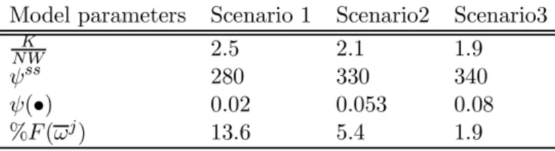
Financial frictions parameters: the financial frictions scenarios are identified according to three primitive parameters: 4) the corporate risk of firms identified by the variance of the idiosyncratic shock $j, 2) the monitoring cost for the bank, c_m, 3) the survival rate of firms, ). The solution of the contract in the steady state will lead to values for the 4) elasticity of external

finance premium to collateral, #(•), 2) net wealth ratio or leverage ratio, _NWK , in steady state, 3) the externalfinance premium in the steady state, #ss (this will be defined in annual basis points), 4) the optimal cut-o value $j and consequently the default probability F($j). The elasticity of the external finance premium to collateral also plays a role in determining the sensitivity of the borrowing limit to financial conditions.

The asymmetries between the two countries will be build up by assuming three dierent

financial scenarios for the foreign country given one particular scenario for the home country. All the three primitive parameters are crucial in order to define a financial scenario. The monitoring costs is a measure of the loan losses and the bankruptcy costs that a bank incurs by giving a loan to a defaulting firm. The distribution and the moments of the idiosyncratic shocks are necessary to define the degree of riskiness for investment projects. The survival rate offirms is an indicator of the riskiness of the financial systems as a whole since it describes the aggregate evolution of the business sector. A very fragile system in the foreign country is identified by a situation in which monitoring costs for banks, perceivedfinancial risk and exit ratio forfirms are high. In the solution to the financial contract this leads to high values for the elasticity and the steady state value of the external finance premium, low leverage, high default probability. Finally low leverage and high elasticity of external finance premium to collateral determine a tighter a borrowing limit and a lower return on asset.

The parametrization strategy40 is based on the following criterion: I set the monitoring costs using as reference the micro data presented before on bankruptcy costs, I keep the default probabil-ity asfixed and then I set the volatility so as to get an external finance premium that corresponds to the value found in the data for the dierence between the rate on Treasury bill and the prime lending - i.e. a value of 200 basis point for the US economy -. The following tables 4,2, show the

40_{Thefirst order conditions for the contract are three equations in three unknwons. One needs to specify the three} primitive parameters to get the three unknowns. There are infinite combinations of these values. Mainly those three situations can arise: a) Both the monitoring cost and the volatility of the idiosyncratic shocks increase and as a result the externalfinance premium and its elasticity increase. b) Only the monitoring cost increases while the volatility of the idiosyncratic shock remainsfixed or decreases. As a result both the externalfinance premium and its elasticity increase. c) Only the volatility of the idiosyncratic shock increases while the monitoring cost remainsfixed. As a result the externalfinance premium and its elasticity increase.

Several other combinations can be derived, but the main message is that it is enough an increase in the monitoring cost to get an increase in the externalfinance premium and in the sensitivity of the business cycle.

Table4: Financial Scenarios for Primitive Parameters.

Primitive parameters Scenario4 Scenario2 Scenario3

_/j 0.26 0.28 0.30

c_m 0.05 0.42 0.3

) 0.973 0.973 0.973

Table 2: Financial Scenarios for Financial Contract Parameters in The Steady State.

Model parameters Scenario 4 Scenario2 Scenario3

K

NW 2.5 2.4 4.9

#ss _{280 330 340}

#(•) 0.02 0.053 0.08 %F($j) 43.6 5.4 4.9

parametrization for three possible financial scenarios for the foreign country given the a baseline parametrization with low externalfinance premium for the home country.

Exogenous shocks: The persistence of the shocks varies between 0.8 and 0.9. The volatility of the shock is calibrated to get output volatility that are close to the ones in the data for the US and the Euro area.

The equilibrium of the model is characterized as the solution of the system of expectation dierence equations of the loglinearized form41. For a solution of the steady state of the model see

Appendix 9. Finally Appendix 10 will provide a definition of the competitive equilibrium in this

case and a brief outline of the loglinearized version of the model.

6

Financial Asymmetries with Identical Policies

The model can now answer the following questions: Do countries show dierential business cycle

fluctuations given dierences in the financial system? If so, under which conditions are those dif-ferential responses more pronounced? The answer to these questions highlights the international

41_{The loglinearized system can be described by a general homogenous matrix equation:}

Et n

X

i=3m

AiXt+i= 0, tD0

wheremis the number of leads,nis the number of lags,Aiare the structural coecient matrices, andAn(n= 1)

is not full-rank. I apply the solution method developed by Anderson and Moore (1985) which enables us to deal with possibly singular systems, unlike the Blanchard-Khan (1980).

business cycle properties of the model and the transmission mechanism generated in this new set-up. To isolate the eect of asymmetries the following analysis assumes identical policies and dierent type of shocks - i.e. asymmetric, symmetric, uncorrelated and correlated. I will consider productiv-ity42 and financial shocks - i.e. shocks to the cost of the loan43 or to net worth44. To examine the impact of financial dierences the discussion will proceed according to the following steps. First, I explore the case of two countries with symmetric financial systems and asymmetric shocks; this allows me to clarify the intuition behind the transmission mechanism in the model. Secondly, I show the main result that business cycle heterogeneity occurs under independent policies. Third I perturb the economy with respect to the benchmark case by considering dierent monetary regimes and dierent degree of openness to completely assess the role offinancial dierences under alterna-tive set-ups. Finally I discuss some properties of the international transmission mechanism mainly referring to the pattern of exchange rates.

Productivity and Financial Shocks With Taylor Rules. Ifirst describe for an illustrative purpose

the mechanism of the model when both countries have the same degree of financial fragility and a positive technology shock hit the home economy. In figure 2 domestic output increases, domestic inflation decreases and this induces via a Taylor rule a decrease of nominal and real interest rates. The consequent reduction in the external finance premium also improves financial conditions by increasing investment, net wealth and price of capital in the home country. The foreign country experiences real and financial eects too. Part of the transmission is explained by a demand eect already present in the previous literature called switching expenditure eect. The decrease in domestic inflation shifts demand in the home country in favor of domestic goods. The decrease in foreign goods demand also reduces foreign inflation and foreign output45. The demand eect generates a negative correlation of output between the two countries. The combination of the switching expenditure eect and of a conventional financial accelerator eect produces an indirect

financial spillover from the home to the foreign country. Indeed given the decrease in foreign

inflation, foreign nominal interest rates decrease as a consequence of the endogenous response of monetary policy. The decrease in the nominal interest rate and consequently in the cost of the loan improvesfinancial conditions and generates an asset price boom in the foreign country. Depending on its magnitude thefinancial spillover eect can partly or completely oset the negative influence of the shift in demand. Thefinancial spillover that is missing in traditional models of international

42_{A productivity shocksA(s}t_{) agects the production of the economy (Y(s}t_{) =A(s}t_)K13k_(st_)Nk_(st_{)) and follows}

an AR(1) process of the type: A(st) =4A(st31) +0_A.

43_{These shocks can be generated by revisions in expectations or confidence crisis. The shock in the model will be} represented as a permanent shock to the cost of externalfinance.

44_{These shocks can be generated by defaultingfirms and induce wealth movements between the two types of agents.} In the model the shock is represented by a permanent shock to the evolution of net wealth.

45_{Theabsorption egect,that increases domestic demand due to increase in income, seems to be negligible since in} this model the increase in output is more likely to generate an increase in investment expenditure than an increase in the consumption of workers.

business cycle can explain why an increase in total factor productivity for one of the two countries can generate an increase in asset prices for the foreign country46.

If the two countries show dierent degrees of financial sensitivity dierential responses occur. Since the credit channel accounts for the transmission mechanism of this model business cycle

fluctuations tend to diverge when higher dierences in the financial system emerge. In particular when the foreign country is relatively more fragile foreign variables are relatively more volatile and persistent. Table 7 and 8 show a systematic comparison of cross-country correlations of output for dierent type of productivity and financial shocks - i.e. asymmetric, symmetric, uncorrelated and correlated - and with increasing dierences in financial system (from scenario 4 to scenario 3). A negative relation emerges between output fluctuations and dierences in financial system. When shocks are correlated the negative relation is stronger under financial shocks. With asymmetric shocks the model is able to reproduce a wide range of correlation values - i.e. from positive to negative - depending on the degree of dierence between financial systems. Contrary to tradi-tional models of the open economy literature where asymmetric shocks always generate negative correlations in output the present model shows that positive correlation might occur when fi nan-cial systems are very close. This is due to the fact that when borrowing constraints have the same strength the positive eect due to the indirect financial spillover is able to oset the

nega-tive switching expenditure eect. This result is more consistent with the data that show positive

correlations of output for countries with similar financial systems even with asymmetric shocks.

Remark 4 The correlation among the business cycles of two countries is a decreasing function of

the degree of financial diversity.

Economic Openness. An increase of the trade intensity produces dierent eects according to

the type of shock, productivity versusfinancial shock. With productivity shock an higher degree of openness induces positive correlation of cycle mostly under asymmetric shocks (see table 7). The intuition of this results can be followed by looking at the eects of a positive technology shock in the home country. With higher economic openness there is an higher decrease in inflation for the foreign country due to the switching expenditure eect. The decrease in inflation generates a decrease in interest rates and boosts the foreign economy too through the increase in investment.

With a shock to the cost of the loan higher trading intensity leads to reduction in the correlation of cycles up to negative values, see table 8. Following a decrease in the cost of the loan in the home country, domestic output and inflation increase. Since inflation in the foreign country increases, the foreign interest rate increases and consequently financial conditions worsen. The increase in domestic output is then associated with a decrease in foreign output due to a decrease in investment. When trading intensity increases the increase in foreign inflation and consequently the decrease in foreign investment and output are higher.

Remark 2 A higher degree of economic openness enhances asymmetries in cycles between the

two countries given the presence of structural dierences in financial systems and with financial

shocks. On the other side higher degrees of trading intensity increase the correlation of cycles when productivity shocks occur.

The persistence of the real exchange rate increases when financial dierences increase. When

simulating a symmetric and correlated productivity shock the persistence of real exchange rate goes from 0.76 in scenario4to 0.82 in scenario 2 to 0.87 in scenario 3. The value of the persistence of real exchange rate between Europe and US is about 0.8347. Since scenario 2 approximate closely the parametrization for US and Europe, the numbers generated by the calibrated model resemble pretty much the numbers in the data. As noticed in Chari,Kehoe and McGrattan sticky price models were not able to generate enough persistence to match the one shown in the data48. The introduction of financial frictions and financial dierences in this model seems to help in this direction. The intuition for the result of the present model can be found in the persistence associated with the real interest rates. Borrowing constraints on investment increase persistence of real interest rates. If the foreign country suers of tighter borrowing constraints the foreign interest rate is relatively more persistent. The real exchange rate will then absorb the dierence in the persistence of the interest rates between the tow countries through the uncovered interest rate parity.

Remark 3 Persistence of real exchange rates increases when financial dierences increase.

A weakness of the insulation property of exchange rates emerges in this setting. The exchange rate works like a shock absorber and shows dierential responses, but this does not prevent either country by having more pronouncedfluctuations when higher dierences infinancial system occur. Figure 3, shows impulse responses of home and foreign variables with a positive foreign shock to net worth. The improvement in the financial wealth increases output, demand and inflation for the foreign country. On impact, output and financial variables are more responsive when the foreign country is characterized by increasing values of elasticity of external finance premium. A higher level of persistence arises when thefinancial system is more stable. This is due to the higher persistence of inflation and interest rates. The home country gets a positive burst from the favorable switching eect even though the increase in output is partly depressed by an increase in inflation and interest rate that adversely aectsfinancial conditions and consumption. Consumption shows a non-stationary pattern since there is a movement of wealth from workers to entrepreneurs.

Remark 4 The insulation property of exchange rates is weakened by financial dierences. 47_{See Chari, Kehoe and McGrattan (2001).}

48_{Statistics presented in Chari, Kehoe and McGrattan (2001) show that sticky price models can generate values for} the persistences of the real exchange rate that go from 0.48 to 0.70 depending on alternative assumptions for untility and international asset markets.