Characterization of pollutant emissions and fuel use for CNG transit buses

(1)

CHARACTERIZATION OF POLLUTANT

EMISSIONS AND FUEL USE FOR CNG TRANSIT

BUSES

By

CHUANHAI ZHU

Bachelor of Science in Environmental Science and

Engineering

Tianjin University

Tianjin, China

2011

Submitted to the Faculty of the

Graduate College of the

Oklahoma State University

in partial fulfillment of

the requirements for

the Degree of

DOCTOR OF PHILOSOPHY

May, 2015

(2)

ii

CHARACTERIZATION OF POLLUTANT

EMISSIONS AND FUEL USE FOR CNG TRANSIT

BUSES

Dissertation Approved:

Dr. Michael Phil Lewis Dissertation Adviser Dr. John N. Veenstra

Dr. Dee Ann Sanders

Dr. Yongwei Shan

(3)

iii

Name: Chuanhai Zhu

Date of Degree: MAY, 2015

Title of Study: CHARACTERIZATION OF POLLUTANT EMISSIONS AND FUEL

USE FOR CNG TRANSIT BUSES

Major Field: CIVIL ENGINEERING

Abstract:

Transit agencies have historically relied on diesel buses to move their passengers; however, many agencies have adopted alternative fuels such as compressed natural gas (CNG). New knowledge is needed to accurately assess the environmental impacts of CNG as a transportation fuel. The goal of this research is to characterize the air pollutant emissions and fuel use of CNG buses. This dissertation focuses on real-world data collection of emissions and fuel use rates and vehicle activity data for CNG buses. The case study fleet included five big capacity (32-seat) CNG buses and five small capacity (19-seat) CNG buses, and three (27-seat) diesel buses. The diesel bus data was used as a baseline to compare the environmental impacts of CNG buses. The central

component of the field data collection process was a portable emissions measurement system (PEMS). Monitored pollutants included carbon dioxide (CO2), hydrocarbons (HC), carbon monoxide (CO), and nitrogen oxides (NOx). Vehicle activity data included, engine speed in revolutions per minute, intake air temperature, manifold absolute pressure, engine load and vehicle speed. The major outcome of the research is new knowledge that may lead to improved environmental and fleet management practices as well as improved decision making capacity for stakeholders.

(4)

iv

3.1.2. Instrumentation Description ... 19

3.1.3. Field Data Collection ... 21

3.1.4. Emissions Rates and Vehicle Activity Data ... 22

3.2. Comparison of Emissions and Fuel Use Rates ... 23

3.2.1. Comparison Bases ... 23

3.2.2. Comparison Approaches ... 26

3.2.2.1. CNG vs. Diesel Comparison ... 26

3.2.2.2. Operational Modal Comparison ... 26

3.2.2.3. Engine Modal Comparison ... 28

3.3. Emissions and Fuel Use Predictive Models ... 31

3.3.1. Correlation Matrix ... 31

3.3.2. Prediction Models using Multiple Linear Regression (MLR) ... 31

3.3.3. Model Validation ... 33

INTRODUCTION ... 1

I.

LITERATURE REVIEW ... 5

II.

METHODOLOGY ... 18

III.

(5)

v

Chapter

Page

3.3.4. Variable Impact Analysis ... 34

3.4. Emissions Inventory ... 34

3.4.1.Annual Fuel Use ... 35

3.4.2. Estimated Annual Emissions ... 35

4.1.1. Field Data Collection ... 37

4.2.1. CNG vs. Diesel Comparison ... 44

4.2.2. Operational Modal Comparison ... 47

4.2.3. Engine Modal Comparison ... 54

4.3.1. Correlation Matrix ... 62

4.3.3. Model Validation ... 69

4.3.4. Variables Impact Analysis ... 76

5.1.1. Field Data Collection ... 83

5.2.1. CNG vs. Diesel Comparison ... 84

5.2.2. Operational Modal Comparison ... 85

5.2.3. Engine Modal Comparison ... 86

5.3.1. Correlation Matrix ... 87

5.3.3. Model Validation ... 89

5.3.4. Variables Impact Analysis ... 89

RESULTS ... 37

IV.

CONCLUSIONS ... 83

V.

RECOMMENDATIONS AND FUTURE WORK ... 90

VI.

(6)

vi

Chapter

Page

REFERENCES ... 92

(7)

vii

LIST OF TABLES

Table

Page

Table 1.1 Top Ten Countries with the Largest NGVs Fleets ... 2

Table 2.1 Summary of Previous Emissions Study with Different Data Collection Methods ... 12

Table 2.2 Summary of Previous Emissions Modeling using Different Approaches ... 17

Table 3.1 Vehicle Information ... 19

Table 3.2 Axion RS+ Pollutant Measurement Instruments Specifications ... 20

Table 4.1 Data Collection Summary ... 38

Table 4.2 Summary Statistics for Big CNG Buses ... 40

Table 4.3 Summary Statistics for Small CNG Buses ... 41

Table 4.4 Summary Statistics for Diesel Buses ... 42

Table 4.5 Tukey Test Results for Big CNG Buses ... 43

Table 4.6 Mass per Time Emissions and Fuel Use Rates ... 44

Table 4.7 Mass per Fuel Used Emissions and Gallon per Time Fuel Use Rates ... 45

Table 4.8 Summary of Percentage of Time per Operational Mode ... 47

Table 4.9 Percentage of Time per Engine Mode for Big CNG Buses ... 55

Table 4.10 Mass per Time Fuel Use Rates (g/s) per Engine Mode for Big CNG Buses ... 58

Table 4.11 Summary of Average Mass per Time Fuel Use Rates per Engine Mode ... 58

Table 4.12 Weighted Average Mass per Time Emissions and Fuel Use Rates for Bus 1 ... 61

(8)

viii

Table

Page

Table 4.14 Summary of Total Weighted Average Mass per Time Emissions and Fuel Use Rates61

Table 4.15 Big CNG Average Correlation Matrix ... 64

Table 4.16 Small CNG Average Correlation Matrix ... 64

Table 4.17 Diesel Average Correlation Matrix ... 64

Table 4.18 Stepwise Selection and VIF Test for Bus 1 CO2 MLR Model ... 65

Table 4.19 Summary of MLR Models for Big CNG Buses ... 66

Table 4.20 Summary of MLR Models for Small CNG Buses ... 67

Table 4.21 Summary of MLR Models for Diesel Buses ... 68

Table 4.22 Summary of Model Validation for Big CNG Buses ... 74

Table 4.23 Summary of Model Validation for Small CNG Buses ... 75

Table 4.24 Summary of Model Validation for Diesel Buses ... 76

Table 4.25 Variables Impact Results for Big CNG Buses ... 77

Table 4.26 Variables Impact Results for Small CNG Buses ... 78

Table 4.27 Variables Impact Results for Diesel Buses ... 79

Table 4.28 Operation Hour and Fuel Use Data of Diesel Fleet ... 80

Table 4.29 Annual Emissions and Fuel Use of Diesel Fleet ... 81

Table 4.30 Annual Emissions Estimation of CNG Fleet ... 82

(9)

ix

LIST OF FIGURES

Figure

Page

Figure 2.1 Diagram of Dynamometer Test Laboratory ... 6

Figure 2.2 Schematic of the Experimental Set-up for Road Method ... 8

Figure 2.3 Schematic Diagram for Montana System ... 10

Figure 2.4 Passenger Cars Installed with Axion ... 11

Figure 3.1 PEMS Work Process ... 22

Figure 4.1 Comparison of Average Mass per Fuel Used Emissions Rates ... 46

Figure 4.2 Average Mass per Time Emissions and Fuel Use Rates per Operational Mode ... 49

Figure 4.3 Average Mass per Fuel Used Emissions Rates per Operational Mode ... 51

Figure 4.4 Average Mass per Distance Emissions and Fuel Use Rates per Operational Mode ... 52

Figure 4.5 Distribution of Time, Emissions and Fuel Use on Each Operational Mode... 54

Figure 4.6 Average Percentage of Time per Engine Mode ... 56

Figure 4.7 Percentage of Time, Mass per Time Emissions and Fuel Use Rates vs. Engine Modes for Bus 1 ... 57

Figure 4.8 Average Mass per Time Emissions and Fuel Use Rates per Engine Mode ... 60

Figure 4.9 Residual Plots of Bus 1 CO2 MLR Model ... 69

Figure 4.10 Model Validation for MLR of Emissions and Fuel Use Models of Bus 1 ... 71

Figure 4.11 Model Validation for MLR of Emissions and Fuel Use Models of Bus 7 ... 72

(10)

1

CHAPTER I

INTRODUCTION 1.

1.1. Background

Transit agencies have heavily relied on diesel buses to move their passengers; however, this is changing considering energy and environmental issues. Many agencies are now moving away from diesel to adopt cleaner, cheaper and more efficient alternatives, such as biodiesel, methanol, chemically stored electricity, propane, liquefied natural gas (LNG), and compressed natural gas (CNG). CNG is the focus of this dissertation.

As an alternative fuel, CNG has several potential advantages: (1) CNG emits significantly lower quantities of some pollutants; (2) Compared with other hydrocarbon-fuel vehicles, Natural Gas Vehicles (NGVs) spend less on maintenance; and (3) NGVs cause fewer problems with spark plugs. Furthermore, the fuel economy, power and acceleration of NGVs are comparable with the conventional vehicles.

(11)

2

The benefits of CNG contribute to the worldwide distribution of NGVs. According to Natural Gas Vehicles Global (NGV Global, 2012), there are roughly 16,700,000 NGVs and 21,000 natural gas fueling stations around the world. Table 1.1shows the top ten countries with the largest NGVs fleets. According to Natural Gas Vehicle for America , natural gas powers about 142,000 vehicles on roads in the United States. Although these vehicles are less than 1% of worldwide NGVs, the use of NGVs in the United States is increasing, especially for transit buses. Use of natural gas (compressed, liquid, or blends) in transit bus fleets began increasing in the late 1990s, growing from 2.8% of buses in 1996 to 18% in 2009. American Public Transportation Association (APTA, 2010) indicates that natural gas-powered buses accounted for 26% of the new buses ordered by transit agencies in 2009. Currently, transit buses are the largest users of natural gas for vehicles in United States.

Table 1.1 Top Ten Countries with the Largest NGVs Fleets (NGV Global, 2012)

Country NGV Population Percentage of NGVs in World Iran 3,000,000 18.8% Pakistan 2,900,000 18.8% Argentina 2,140,000 12.5% Brazil 1,739,676 11.2% China 1,577,000 6.6% India 1,250,000 7.2% Italy 746,470 5.1% Ukraine 390,000 2.6% Colombia 380,000 2.3% Thailand 358,000 2.0% 1.2. Problem Statement

Previous studies about exhaust emissions of CNG transit buses are limited in number and scope. Many of these studies focused only on the fuel economy and fleet managements issues. The major goal of this study is to characterize the emissions and fuel use of CNG transit buses. CNG

(12)

3

emissions and fuel use were compared to a baseline of diesel bus emissions and fuel use. The major output of this study is a case study comparing CNG versus diesel emissions and fuel use for transit buses. The major outcome of the case study is new knowledge that leads to improved environmental and fleet management practices as well as improved decision making capacity for stakeholders.

1.3. Scope

The foundationof this study was the transit bus fleet owned by Oklahoma State University (OSU), which serves the university and the surrounding Stillwater community. This bus fleet provides transit service from 6:20 a.m. to 10:30 p.m., Monday through Friday, throughout the academic year, with three on-campus routes and six off-campus routes. The stops vary depending upon demand (OSU, 2014).

The OSU fleet consists of 19 CNG transit buses, which include ten 2009 Ford E450 and nine 2010 El Dorado buses. There are seven diesel buses (2003 Blue Bird) that remain from the previous diesel fleet that were used prior to the switch-over to the current CNG fleet. These diesel buses are only used on “trail” routes to transport the overflow passengers or operate on routes when CNG buses are out of service for maintenance.

This study is unique in that it is based on real-world data instead of engine dynamometer data collected in a laboratory. The real-world emissions and fuel use data for each bus was collected by a portable emissions measurement system (PEMS) while the bus drove on its scheduled route. Emissions and fuel use measurements were taken on the diesel buses as well to establish an emissions and fuel use baseline for the original diesel fleet. Emissions and fuel use of the current CNG bus fleet and the previous diesel bus fleet were compared in order to assess the emissions and fuel use advantages (or disadvantages) of CNG versus diesel for transit bus fleet. There were

(13)

4

four gas pollutant emissions measured and analyzed in this study, which are carbon dioxide (CO2), hydrocarbons (HC), carbon monoxide (CO), and nitrogen oxides (NOx).

1.4. Objectives

The major goal of this study is to characterize pollutant emissions and fuel use of a CNG transit bus fleet. In order to accomplish this goal, the following objectives were completed:

1. Collect real-world emissions, fuel use, and engine performance data for CNG and diesel buses;

2. Compare emissions and fuel use of CNG buses versus diesel buses;

3. Identify the relationships between emissions, fuel use, and engine performance data for CNG and diesel buses;

4. Develop emissions and fuel use predictive models for CNG and diesel buses; and 5. Develop emissions inventory for the CNG fleet and the old diesel fleet.

The specific outcomes of the study include:

1. A robust dataset of real-world emissions, fuel use, and engine performance data for CNG and diesel transit buses;

2. A comparison of the results and relationships between emissions, fuel use, and engine performance data for CNG and diesel buses;

3. A set of predictive models for emissions and fuel use for CNG and diesel buses; and 4. A emissions inventory for the CNG fleet and the old diesel fleet.

(14)

5

CHAPTER II

LITERATURE REVIEW

2.

The body of literature related to CNG and diesel bus emissions and fuel use is limited in scope and nature; however, there are several studies related in a tangential manner. This section addresses previous work related to the objectives of this study, specifically data collection methods, emissions comparison approaches, and emissions predictive modeling techniques. 2.1. Data Collection Methods

Several methods have been utilized to measure mobile source pollutants. In this section, three testing methods related to this study are explained. These methods include engine dynamometer testing, remote sensing and portable emissions measurement system (PEMS).

2.1.1. Engine Dynamometer Testing

Engine dynamometer testing is widely used to estimate and quantify air pollutant emissions. In this type of test, only the engine, not the entire chassis, is set in a laboratory with test instruments. Emissions data and engine data are collected while the engine operates in several steady-state

(15)

6

modes. The modes are usually classified by specified constant speed or engine loads (Abolhasani et al., 2008).

Dynamometer testing is a popular approach for transit bus research. For instance, Serrano et al. (2012) used dynamometer tests to study the impacts of biodiesel on buses engine. The test bench was equipped with a Schenk hydraulic dynamometer as shown in Figure 2.1. The test engine was also connected with an exhaust gas analyzer for emission data, as well as a fuel use measurement device for fuel use data. A control system was used to avoid the impacts of technician

intervention. Emission rates of NOx and engine performance parameters (RPM and Torque) were measured while the engine was fueled with seven different biodiesel fuels. The engine ran following the European Transient Cycle (ETC) during data collection. The results quantified the emissions and fuel use benefits of biodiesel blends on bus engines.

(16)

7

Dynamometer tests also played an important role in the development of several emissions estimator models. For non-road equipment, the United States Environmental Protection Agency (EPA) developed the NONROAD model based on the data collected from eight-mode

dynamometer tests. MOBILE was developed to predict the emissions of on-road mobile sources, such as cars, buses, trucks and motorcycles. Another model for on-road vehicles was Motor Vehicle Emission Simulator (MOVES), which was developed to replace MOBILE in 2004. As with NONROAD, both MOBILE and MOVES used the data collected from dynamometer tests as their primary resources.

Dynamometer tests do not always represent real-world situations since it is based only on engine data rather than whole vehicle activity. Moreover, some factors cannot be simulated in the laboratory, such as pavement and traffic conditions. Considering these shortcomings, other technologies have been developed in order to obtain emissions and fuel use data that mimics the real-world data. Nevertheless, dynamometer tests are still a common method for emissions research, especially when engine operations follow a fixed cycle.

2.1.2. Remote Sensing

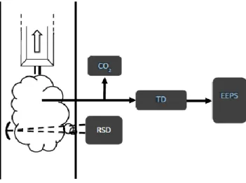
Remote sensing technology is a viable option for collecting real-world emissions data from vehicles. The remote sensing devices measure gaseous pollutant concentrations in the exhaust plume of vehicles as they run in real-world conditions (SBRC, 1994). Hallquist et al. (2012) developed an experimental method to collect transit bus emissions data using this technology, which was called “Road”. A remote sensing device (AccuSan RSD 3000, Environmental System Products Inc.) was used for measurements of gas pollutants including CO, HC and NOx . CO2 was measured by a non-dispersive infrared gas analyzer (LI-840, LI-COR Inc. 1HZ). Engine Exhaust Particle Sizer Spectrometer (EEPS, Model 3090, TSI Inc.) was used to analyze particular matter (PM). Additionally, to minimize the impacts of ambient temperature on PM measurements, a

(17)

8

thermo denuder (TD; Dekati) was used to heat the exhaust sample flow to 298K before the sample entered the EEPS. These four instruments were set up at one spot along the experimental bus route. Emissions data for pollutants were measured as transit buses passed the test location (Figure 2.2). The goal of this study was to characterize PM and gaseous emissions of a European transit bus fleet, which contained both CNG and diesel buses.

Figure 2.2 Schematic of the Experimental Set-up for Road Method (Hallquist, et al., 2012)

Compared with dynamometer testing, the emissions data collected by remote sensing instruments more closely resembles real-world data; however, there were still shortcomings for this method. For example, other traffic had a significant impact on the experiment. Since the instruments were set along the transit bus route, the emissions measurements were affected if other vehicles drove through the test location. In fact, in order to minimize the influence of other traffic, Hallquist et al.(2012) chose bus depots as the experiment locations, although bus depots did not represent the typical and real-world traffic conditions of transit buses. Another shortcoming of remote sensing was that limited data increased the level of variation in the results. Because all the instruments were deployed at one location along the route, the measurements only performed when the buses reached the location. Although each bus was tested three times, the quantity of data was not sufficient to build a database. In order to solve this problem, a chase car was used (Pirjola et al.,

(18)

9

2004), in which an instrumented vehicle followed the test vehicle. Challenges with this approach included how to minimize the influence of emissions from the chase vehicle, and how to keep a constant distance between the chase vehicle and the test vehicle. Furthermore, mass emissions rates could not be determined, since the vehicle’s exhaust flow rate was unknown and detailed vehicle activity was generally not known such as MAP, engine speed (RPM) and engine load, which dramatically affected emissions.

2.1.3. Portable Emissions Measurement System (PEMS)

Another advanced technology used for vehicle emissions studies is on-board portable emissions measurement system (PEMS). PEMS is usually contained in a carry-on luggage-size case. The PEMS is installed on the tested vehicle in advance, and then it collects emissions data on a second-by-second basis as the vehicle travels its real-world route. Simultaneously, engine activity data is measured and transmitted to the PEMS as well.

Several researchers have employed PEMS to study exhaust emissions from different types of vehicles, such as construction equipment, passenger cars, and transit buses. Frey (2010) and his North Carolina State University research team (Rasdorf et al., 2012; Lewis et al., 2009; and Aholhasani et al., 2008) conducted several research projects about emissions of construction equipment. For instance, Frey et al. (2010) developed a methodology for collecting and analyzing real-world in-use data from non-road construction equipment. Rasdorf et al. (2012) conducted a case study to identify construction activities that caused the most emissions and fuel use on a construction project. Lewis et al. (2009) developed a methodology for estimating weighted-average emission rates and fuel uses of construction equipment performing representative duty cycles. Abolhasani et al. (2008) characterized real-world emissions, fuel use, and engine activity for excavators. This research used the data collected by a PEMS, the Montana Universal System,

(19)

10

which was manufactured by Clean Air Technology International (CATI). A schematic of this system is shown in Figure 2.3.

Besides Frey and his research team, Lee et al. (2012) conducted a study for the Texas A&M Transportation Institute (TTI) to compare vehicular emissions from real-world in-use PEMS test to the EPA emissions estimation model MOVES. Another recent PEMS system manufactured by CATI was the Axion. TTI used the Axion to collect real-world emissions data from a 1999 Dodge Grand Caravan. As seen in Figure 2.4, probes and hoses were installed on the test vehicle and connected to its tailpipe (left); the exhaust samples were sent to the Axion main unit (right), and during measurement, the emissions data displayed on the unit’s screen on a second-by-second basis.

(20)

11

Figure 2.4 Passenger Cars Installed with Axion (Lee et al., 2012)

Similarly, TTI used a PEMS for data collection on another research project related to the analysis of school bus emissions and activity data (TTI,2006). Five diesel school buses fueled with two types of diesel fuel, representing a sampling of the Texas fleet, were tested. Based on the

collection and analysis of exhaust emissions and operating data, this project determined operating profile modification, fuel formulations and emissions control techniques of school bus fleets in Texas.

Compared with the previous methods, there are several advantages of PEMS, (1) capability of collecting real-world data; (2) second-by-second data collection during the experiment, which provides enough data for statistical analysis; (3) capability of collection of corresponding engine performance data on a second-by-second basis, and (4) easy set-up on test vehicles.

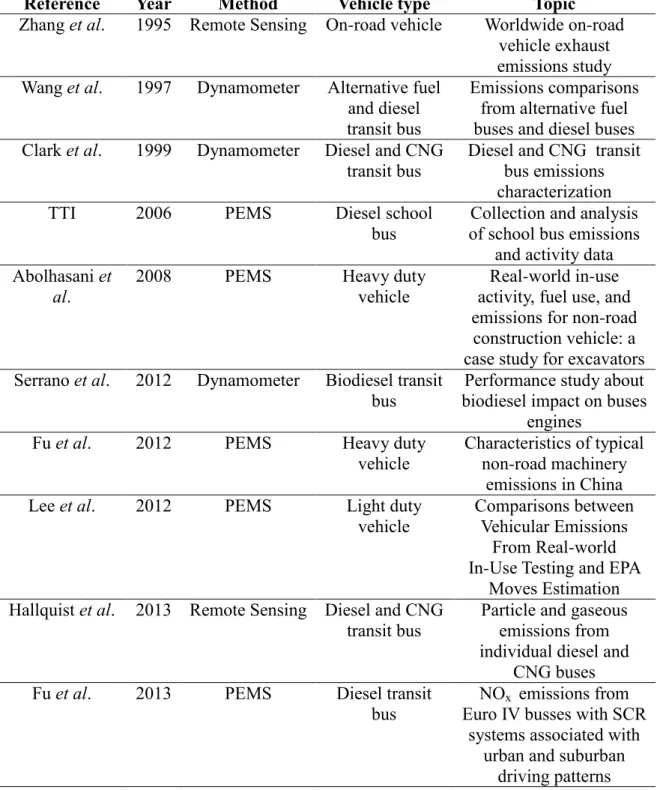
The three data collection methods were widely used on different mobile sources for different emissions research topics. Table 2.1 summarizes some previous emissions studies using these data collection methods including the references, year, test vehicle type, and research topics.

(21)

12

Table 2.1 Summary of Previous Emissions Study with Different Data Collection Methods

Reference

Year

Method

Vehicle type

Topic

Zhang

et al

.

1995 Remote Sensing On-road vehicle

Worldwide on-road

vehicle exhaust

emissions study

Wang

et al

.

1997

Dynamometer

Alternative fuel

and diesel

transit bus

Emissions comparisons

from alternative fuel

buses and diesel buses

Clark

et al

.

1999

Dynamometer

Diesel and CNG

transit bus

Diesel and CNG transit

bus emissions

characterization

TTI

2006

PEMS

Diesel school

bus

Collection and analysis

of school bus emissions

and activity data

Abolhasani

et

al

.

2008

PEMS

Heavy duty

vehicle

Real-world in-use

activity, fuel use, and

emissions for non-road

construction vehicle: a

case study for excavators

Serrano

et al

.

2012

Dynamometer

Biodiesel transit

bus

Performance study about

biodiesel impact on buses

engines

Fu

et al

.

2012

PEMS

Heavy duty

vehicle

Characteristics of typical

non-road machinery

emissions in China

Lee

et al

.

2012

PEMS

Light duty

vehicle

Comparisons between

Vehicular Emissions

From Real-world

In-Use Testing and EPA

Moves Estimation

Hallquist

et al

. 2013 Remote Sensing Diesel and CNG

transit bus

Particle and gaseous

emissions from

individual diesel and

CNG buses

Fu

et al

.

2013

PEMS

Diesel transit

bus

NO

x

emissions from

Euro IV busses with SCR

systems associated with

urban and suburban

(22)

13 2.2. Emissions Comparison

Several technologies for emissions reductions have been developed and used on mobile sources, such as alternative fuels and after-treatment devices. In order to evaluate their benefits, emissions rates resulting from these reduction technologies are quantified and compared to the vehicles without reduction technologies. This section introduces common comparison approaches applied to transit bus studies.

Hallquist et al. (2012) tested particles and gaseous emissions from diesel and CNG buses. A remote sensing method was applied to collect data from a European fleet with 28 diesel and seven CNG buses. The instruments measured the gaseous pollutants and particle concentrations of the exhaust samples, and fuel use was estimated based on the CO2 concentration. Based on

concentrations, sample flow, and fuel use, the emission rates of each pollutant (PM, CO2, CO, HC and NOx ) were calculated on mass per distance or fuel used basis and then compared with the road vehicle emission model HBEFA 3.1.

Fu et al. (2013) used PEMS collected NOx emission data from Euro IV buses to determine the impacts of Selective Catalytic Reduction (SCR) systems on NOx emission rates. The NOx emission rate comparison was made between buses with and without SCR, on mass per distance basis. Since vehicle speed was highly correlated with SCR work efficiency and NOx emission rate, the comparison was separated in different speed modes.

Jayaratne et al. (2009) monitored exhaust emissions from 13 CNG and nine diesel transit buses on a chassis dynamometer. PM10, CO2，and NOx were measured under four identical conditions, which were 0% (idle), 25%, 50% and 100% of the maximum engine power. Emissions of idle mode were presented on mass per time basis, and emissions of other three modes were compared on mass per distance basis for each pollutant between CNG and diesel buses.

(23)

14

Zhang et al. (2014) characterized real-world fuel use and CO2 emissions for a transit bus fleet, containing diesel, CNG, LNG and hybrid buses, based on the 30 min on-board data obtaining by PEMS for each bus. The fuel use rate and CO2 emission rate of each type of bus were compared on mass per distance basis. Also, the traffic patterns were separated in 16 modes by speed

distributions and road conditions. The fuel use rates and CO2 emission rates of all the modes were compared on mass per distance basis for each type of bus.

Texas Transportation Institute (2006) tested five diesel school buses by a PEMS, which

represented a sampling of the Texas fleet. Emissions data included CO, HC and NOx . To quantify route impacts on emissions, the tested buses were required to drive along the rural and urban routes. Emissions of tested buses driving on these two routes were compared on mass per distance basis.

Different comparison approaches were applied in previous studies to achieve different goals: (1) quantify the benefits advanced emission reduction technologies, including alternative fuels (CNG and Bio-diesel) and exhaust gas after-treatment devices (SCR); (2) assess the impacts of engine performances on emission rates such as vehicle speeds and engine loads; (3) estimate the outside influences on emission rates such as road conditions. In these methods, the emission rates were commonly compared in three ways: (1) Mass per time; (2) Mass per distance; and (3) Mass per energy (fuel used). Some of the comparison methods discussed here will be developed and utilized for the dissertation research for the OSU bus fleet.

2.3. Emissions Predictive Models

Several factors have significant impacts on vehicle emissions, such as engine performance and vehicle kinematic variables. Some pollutant emissions even have strong relationships with each other. To quantify these influences, emission predictive models have been developed in previous

(24)

15

studies. This section will highlight approaches applied to build these models, such as regression, weighted average and artiﬁcial neural network (ANN).

Kamarianakis et al. (2013) developed a predictive regression model for particle number (PN) emission rates of diesel buses. Data were obtained from two conventional diesel buses in a Connecticut Transit bus ﬂeet. Several models were built based on engine performance variables, vehicle kinematic variables, vehicle specific power (VSP) and gaseous emissions. A combined model was developed as well, which included kinematic variables, VSP and gaseous emissions as the predictors. Least Absolute Value (LAV) and Ordinary Least Squares (OLS) regression were applied to develop the models. R2 values for each model were presented to assess the precision and appropriateness of the models.

Zhai et al. (2008) applied a discrete modes approach to build emissions predictive models for diesel transit buses. The data were collected from a fleet consisting of 12 diesel buses. The VSP data were separated into eight modes, and the average emission rate of each pollutant in each mode was calculated. Similarly, speed data were divided into five modes to develop other emissions models. Seven buses with available GPS data were contained in this model but not the entire fleet. A comparison between these two models was made to test their predictive power of total trip emissions. The two models were used to predict the total trip emissions of seven buses selected from the fleet. The predicted emissions values were compared with the measured emissions values in order to get the prediction error.

Regression and weighted average models are appropriate when dependent variables (emission rates) show linear relationships with independent variables, such as VSP and Speed. However, sometimes these models do not capture the emissions spikes resulting in low R2 values (Mudgal et al., 2011). ANN approach is often applied because it can handle nonlinearity and has no requirements of assumptions on input data as needed by statistical models.

(25)

16

Mudgal et al. (2011) employed ANN based emissions predictive models for biodiesel transit buses after finding the linear models had low R2 values (maximum of 0.47). The inputs of these models were biodiesel percentage, speed, acceleration, RPM, VSP, passenger count, intake air temperature (IAT), and manifold air pressure (MAP). The outputs included emission rates of CO2, CO, HC, NOx and PM. The data were divided into three parts, 70% for training the models, 15% for validation and the remaining 15% for testing the predictive power of the models. Validation is an important part of ANN, which is used to check and control overfitting of the data. Compared with regression models in the previous example, ANN based models have higher R2 values. Compared with regression and weighted average, ANN can develop more powerful predictive models, especially for nonlinearity. However, the complicated ANN models lead to longer computation time. As a result, regression and weighted average, which have shorter computation time, are more appropriate when the variables have strong linear relationships. Table 2.2

(26)

17

Table 2.2 Summary of Previous Emissions Modeling using Different Approaches

Ref Year Approaches Input Output

Atkinson et al. 1998 ANN IAT, RPM, fuel rack position, engine coolant temperature,

exhaust gas temperature, and fuel

rail temperature and pressure

Instantaneous engine torque, fuel use, exhaust gas

temperature and emissions (CO2, CO, HC and NOx )

Desantes et al. 2002 ANN Engine speed, fuel mass, air mass, fuel

injection pressure, start of injection, EGRa _{and nozzle}

diameter

Emissions (NOx and PM)and BSFC b

Taylor et al. 2004 Weighted average

Emissions data from UDDS c_(CO

2, NOx and PM)

Emissions of other dissimilar driving cycles

(CO2, NOx and PM) Zhai et al. 2008 Weighted

average

VSP, Speed Emissions(CO2, CO, HC and NOx ) Ghobadian et al. 2008 ANN Speed and bio-fuel

blend

Torque, SFC d_{and exhaust} emissions (HC and CO) Mudgal et al. 2011 ANN Biodiesel

percentage, speed, acceleration, RPM, VSP, passenger count, IAT and MAP

Emissions (CO2, CO, HC, NOx and PM)

Lewis et al. 2012 Regression Fuel use Emissions (CO2) Kamarianakis et al. 2013 Regression Engine performance,

vehicle kinematic, VSP, and gaseous emissions

Emissions (PN)

a _{EGR means exhaust gas recirculation rate}

b_{BSFC means brake specific fuel consumption}

c

UDDS means urban dynamometer driving schedule

(27)

18

CHAPTER III

METHODOLOGY 3.

This chapter presents the methodology used to characterize and analyze the emissions and fuel use data of the OSU Bus Fleet. It includes four sections: (1) characterization of OSU bus fleet data, (2) Comparison of emissions and fuel use rates, (3) Emissions and fuel use predictive models, and (4) Emissions and fuel use inventory.

3.1. Characterization of OSU Bus Fleet Data

This section presents the process to create the database of transit bus emissions and fuel use. The experimental instrumentation of a typical PEMS unit is described as well.

3.1.1. Bus Fleet Information

The case study bus fleet belongs to the Oklahoma State University (OSU)-Stillwater Community Transit system. This system provides transit service from 6:20 a.m. to 10:30 p.m., Monday through Friday, throughout the academic year and reduced routes during non-academic months. Two routes are available on campus during the day, and one route is used during the evening and

(28)

19

summer sessions. Off campus, there are five routes during the day and one in the evening. These routes provide service to downtown, dining, and entertainment establishments. The stops may vary depending upon demands. OSU recently transitioned its bus fleet from diesel to CNG. The current fleet consists of 26 buses, including 19 CNGs and seven diesels. The CNG buses include nine 2010 El Dorado (referred to as “Big CNG”) and ten 2010 Ford E450 (referred to as “Small CNG”). The diesel buses were retained from the previous fleet and include seven 2003 Blue Bird (referred to as “Diesel”). The diesel buses are used on “trail” routes to transport overflow

passengers and are placed on fixed routes only when a CNG bus is taken out of service for maintenance. The specifications of the three types of buses are shown in Table 3.1.

Table 3.1 Vehicle Information

Parameter Big CNG Small CNG Diesel

Model Year 2010 2009 2003

Manufacturer E1 Dorado Ford Blue Bird

Model Type Axess E-450 NA

Vehicle Weight(lbs) 42,760 14,500 36,200

Displacement (L) 8.9 6.8 8.3

Cylinders 6 10 6

Transmission Automatic Automatic Automatic

HP @ RPM 320@2,000 305@4,250 300@2,000

Torque @ RPM 1,000@1,300 420@3,250 860@1,300

3.1.2. Instrumentation Description

An Axion RS+ PEMS unit was used for the data collection procedure, which contains several emission measurement instruments. Two non-dispersive infrared (NDIR) analyzers measure three gaseous pollutants concentrations, which are carbon dioxide (CO2), hydrocarbons (HC) and carbon monoxide (CO). HC is non-methane hydrocarbons (NMHCs) since Axion Rs+ measures and reports HC as propane. Two electrochemical sensors (E-Chem) measure nitrogen oxides (NOx ). There is a zeroing instrument built into the Axion software so that while one analyzer (or sensor) is referencing ambient air, the other is still collecting data; this allows continuous and

(29)

20

reliable data collection. For particle measurements, an advanced laser diode forward light scattering sensor can measure the concentration of particulate matter 10 (PM10). However,

particle emissions of both diesel and CNG buses are small size fine particles or ultrafine particles, which are too small to be measured by the laser scatter. Because of this limitation, particle emissions were not included in this study. Table 3.2 shows the specifications of those emission measurement instruments. To ensure data accuracy, the system was calibrated after every 10 hours operation, using Bar 97 low calibration gas (C3H8 203 ppm, CO 0.50%, CO2 6.00%, NO 302ppm).

Table 3.2 Axion RS+ Pollutant Measurement Instruments Specifications

Gas Measurement

Range

Accuracy Resolution Type of

Measurements HC 0-4000 ppm ±8 ppm abs. or ±3% rel. 1 ppm NDIR CO 0.00-10.00% ±0.02% abs. or ±3% rel. 0.001 vol. % NDIR CO2 0.00-16.00% ±0.3% abs. or ±3% rel. 0.01 vol. % NDIR NOx 0-4000 ppm ±25 ppm abs. or ±4% rel. 1 ppm E-Chem PM10 0.00-300 mg/m3 NA 0.01 mg/m3 Laser Scatter

Considering the scope limitation of the laser scatter, only one probe was inserted into the tailpipe of the tested buses to collect exhaust samples for gaseous pollutant emissions measurement (CO2, HC, CO and NOx ). The probe sent the samples through a sample hose to the E-Chem sensors and NDIR analyzers, which were in a luggage-size case (main unit of PEMS). After processing by the PEMS, exhaust samples were removed through the exhaust instrument tubes. The emissions data were transmitted to a system computer, which was also contained in the main unit.

An OBD sensor was connected to the engine in order to measure engine performance data including Revolutions per Minute (RPM), Intake Air Temperature (IAT), Manifold Absolute Pressure (MAP), Engine Load (LOAD), Vehicle Speed (SPEED), air inflow and exhaust flow

(30)

21

rate. The engine data were sent back to the system computer via a RS 232 cable. A global positioning system (GPS) was used to measure global positioning data. All the measured data were combined by the computer and displayed on its screen so that the whole process could be monitored.

3.1.3. Field Data Collection

The data collection procedure was divided into four steps, which were pre-installation,

installation, data collection and decommissioning. At least one hour was needed to set up all of the PEMS instruments. Since transit buses always began service in the early morning, pre-installation was done during the previous evening before the data collection day, when the tested bus was out of service and back at the fueling station.

During the pre-installation step, other accessories were installed. A metal clamp was used to fix the probe to the tailpipe of tested bus. One port of the sample hose was connected to the probe, and the other port was put through the window at the end of the bus, where the main unit was placed. The exhaust tubes were directed out of the same window. The OBD sensor was connected to the engine and the RS 232 table, and the other port of RS 232 was set close to the main unit location.

During the installation phase, the main unit needed at least 30 minutes to warm up at the

laboratory before collecting data. After that, the unit and other accessory equipment were brought on the bus. The main unit was connected with all the accessories placed in pre-installation stage, which were the sample hoses, exhaust tubes and RS 232 cable. The GPS was connected to the main unit as well. An independent battery (12-14DC) was also carried on the bus to supply power for the PEMS.

During the data collection procedure, the following data were collected and displayed on the system computer screen on a second-by-second basis while the bus drove along its route:

(31)

22

pollutant concentrations, engine performance data, and global positioning data. Emissions rates of all pollutants and fuel use rates were calculated by the computer and also displayed on a second-by-second basis. All the data were automatically saved in a txt file. One researcher was required to stay on the bus to monitor the operation of the PEMS during this procedure to ensure that the PEMS unit was functioning properly and also to protect the unit from damage. Figure 3.1 shows the work process of the PEMS during data collection.

After data collection, the researcher on the bus copied the .txt file to a flash drive, shut down the system computer, and disconnected all the accessories. Due to the schedule, the bus usually stopped for 10 to 15 minutes at the Multi-Modal Transportation Terminal. During that period, the researcher removed all equipment from the bus to finish the decommissioning phase.

Figure 3.1 PEMS Work Process

3.1.4. Emissions Rates and Vehicle Activity Data

This section is to present the analytical methods used to estimate real-world emission rates and vehicle activity data of tested buses. The field data was collected from five Big CNG buses (32 seats) and five Small CNG buses (19 seats), and three Diesel buses (27 seats). Summary statistics including maximum (MAX), minimum (MIN), mean (AVG), standard deviation (SD), and

(32)

23

coefficient of variation (CV) - which is the standard deviation divided by the mean, were computed for each pollutant, fuel use, and each engine performance parameter.

Summary statistics were computed for pollutant emissions rates of NOx , HC, CO, and CO2. Fuel consumption rates were also included in this analysis. Summary statistics were computed for common engine performance parameters as well, including revolutions per minute (RPM), manifold absolute pressure (MAP), intake air temperature (IAT), engine load (LOAD), and vehicle speed (SPEED). Summary statistics reveal the central tendencies and variation in the data and permit comparisons of different data categories. It is the first step of data processing, which presents the data characteristics.

3.2. Comparison of Emissions and Fuel Use Rates

Emissions and fuel use of vehicles are usually compared in order to quantify the benefits of advanced alternative fuels and emission reduction technologies, or estimate the influences of vehicle activity. This section briefly presents the comparison bases and approaches involved in this study. Emissions data of all gaseous pollutants (CO2, CO, HC, and NOx) and fuel use data were used for the comparisons.

3.2.1. Comparison Bases

Three common unit bases of emission rate comparisons were used: (1) mass per time; (2) mass per distance and (3) mass per fuel used. The basis of fuel use comparisons is presented as well. 1. Mass per time

The PEMS measures and reports data for emission rates on a gram per second basis (g/s). The average emission rate of each pollutant was compared among all the tested vehicles, and the preliminary findings from this comparison lead to more specific comparisons. This unit basis was also used to make the comparisons among different operational modes and engine modes.

(33)

24

Furthermore, emission rates on a gram per second basis were converted to gram per hour and kilogram per hour basis when they were used for mass per distance and mass per fuel used conversions.

2. Mass per distance

The mass per time emissions rates were converted to mass per distance rates based on the following equation: 𝐸𝐷= 𝐸_𝑇 𝑆 Equation 1 Where: ED=Emission rates (g/km) ET=Emission rates (g/hr) S=Vehicle Speed (km/hr)

Considering the nature of this equation, S (km/hr) cannot be zero. Thus, it was not appropriate to use this equation when a tested bus was idling. Idling emission data need to be removed before the conversion. Furthermore, this equation would have a large value when the bus speed was low. Although the value was reasonable for that second, it could cause bias when calculating the average emission rates for a specific distance. To avoid this bias, average ET (g/hr) and average S (km/hr) were calculated first, and then converted using Equation 1 to get unbiased average ED (g/km) for a period or a route. Mass per distance is a common basis for emission data collected from dynamometer tests. In this study, this basis was used to characterize operation impacts on transit bus emission rates.

3. Mass per fuel used

In order to compare the average emission rates for CNG and diesel fuels, the emission rates were converted to mass per fuel used basis (grams per gallon) using Diesel Gallon Equivalents (DGE). DGE is the amount of alternative fuel it takes to equal the energy content of one liquid gallon of diesel.

(34)

25

A standard unit of measurement for CNG was developed by the National Conference of Weights & Measurements (NCWM). This unit is 1 diesel [US] gallon equivalent (DGE) per 6.31 pounds of natural gas. A CNG to DGE conversion index of 1.257(DGE/hr)/(g/s) was developed with this measurement value. It means that 1.257 DGE of fuel will be consumed per hour if the fuel use output from the PEMS is 1 gram per second. Similarly, based on the diesel density (3.2 kg/gallon), the diesel DGE conversion was developed, which is 1.125 (DGE/hr) / (g/s). Based on the DGE conversion index and fuel use, the emission rates were converted from mass per time to mass per DGE (Equation 2).

𝐸_𝐹 = 𝐸𝑇

𝐹𝐶 × 𝐴 Equation 2

Where:

EF=Mass per fuel used emission rates (kg/DGE)

ET=Mass per time emission rates (kg/hr)

FC=Fuel Consumption (g/s)

A=DGE conversion index; for CNG bus, it is 1.257(DGE/hr)/(g/s); for diesel bus, it is 1.125(DG/hr)/(g/s).

Similar to the mass per distance basis conversion equation, this equation gives large emission rate values when the fuel use is low, which leads to bias in average emission rates. As a result,

average ET (g/s) and average FC (g/s) were calculated first, and then converted using Equation 2 to get unbiased average EF (kg/DGE) for a period or a route. In this study, this basis was used to characterize operation impacts on transit bus emission rates.

4. Fuel use comparison basis

This study also includes three bases of fuel use. The original fuel use data were reported by the PEMS on mass per time basis (gram per second). When presenting the fuel use of a bus in non-idling modes, the original data were converted to mass per distance basis (gram per kilometer) based on the speed data. When comparing the fuel use between different fuel types, according to the DGE conversion index, the fuel use data were converted to gallon per time basis (DGE per hour).

(35)

26 3.2.2. Comparison Approaches

The objective of the comparisons in this study is to: (1) quantify the emissions and fuel benefits of CNG compared with diesel; (2) assess the operational influences on emissions and fuel use rates of tested buses; and (3) estimate the engine activity impacts on emissions and fuel use rates of tested buses. This section presents the approaches used to achieve these goals.

Before the specific comparisons, a summary table was made for the bus fleet, which contains the average emissions and fuel use rate of each tested bus. This table reveals the variability of emissions and fuel use rates among the individual bus, which would be the base to make the specific comparisons.

3.2.2.1. CNG vs. Diesel Comparison

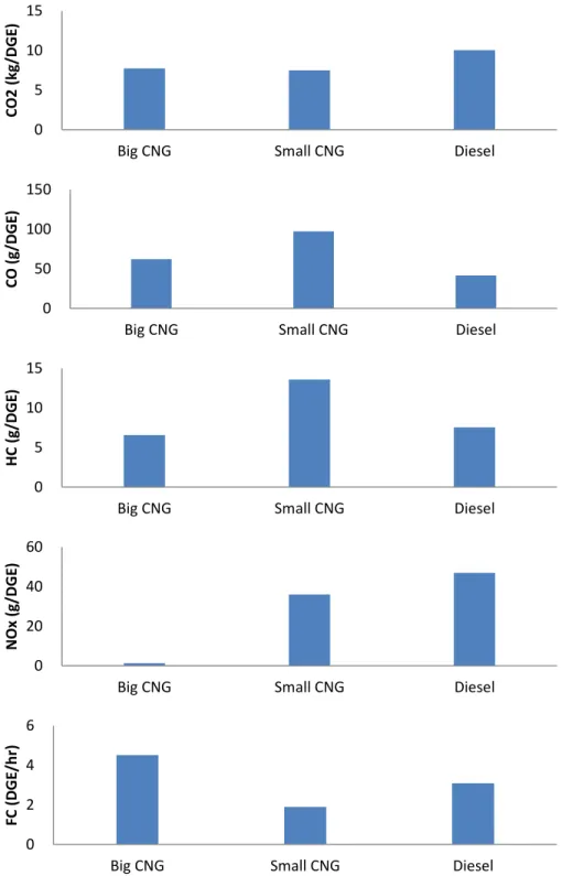
In order to compare the emissions rates between CNG and Diesel fuels, mass per time emissions rates were converted to mass per fuel used rates. A summary table was made containing the average mass per fuel used emissions rates of each tested bus in order to give an overview of the database. Mass per time fuel use rates were also converted to gallon per time rates, and the average gallon per time fuel use rates of all tested buses were added in the summary table. The average mass per DGE emissions rates and DGE per hour fuel use rates of each type of buses were calculated and displayed in the histograms.

3.2.2.2.Operational Modal Comparison

This section presents a method to evaluate the operational impacts on emissions and fuel use rates of all tested buses, with the following steps.

1. Determine operational modes

To assess the operational influence, the operational modes were categorized as idle, cruising, acceleration and deceleration (Frey et al., 2001; 2002). Idle was defined as zero speed and zero

(36)

27

acceleration. To define the acceleration mode, several considerations were included. Firstly, the vehicle should be moving and increasing in speed; therefore, both speed and acceleration must be greater than zero. However, if vehicle speed varied slightly the mode was typically judged as cruising. As a result, in most instances, the acceleration mode needed a minimum acceleration of two mph/sec. Deceleration was defined in a similar manner, but the criteria for deceleration were based on negative acceleration rates. All other situations not classified were classified as cruising. The cruising mode was approximately steady-speed driving but some drifting of speed was allowed. All of the second-by-second data for each tested bus were categorized and separated into these four modes.

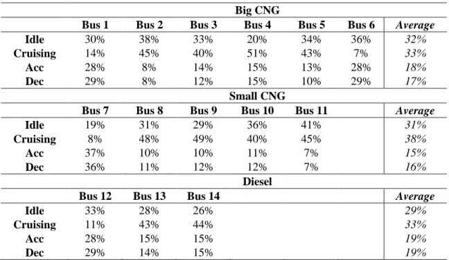
2. Quantify the amount of time spent on each operational mode

The amount of time spent on each operational mode for each tested bus was quantified. Based on that, the fraction of time spent on each mode was also calculated. Furthermore, in order to compare the time distribution among the three types of buses, the average percentage of time spent on each operational mode was calculated for each type of bus.

3. Categorize operational mode data for each tested bus

In order to assess the relative importance of each operational mode, the average emissions and fuel use rates (g/s) of the four modes were calculated for each tested bus. The average emissions rates were also converted from mass per time basis to mass per fuel used basis, and mass per distance basis. Similarly, the average fuel use rates were also converted from mass per time basis to gallon per time basis, and mass per distance basis. All of these values were summarized in the operational mode dataset table for each tested bus. The table also included the amount of time in each mode and the data collection information. All the operational mode analyses were based on these analysis tables.

(37)

28

4. Analyze the relationship between operational modes and emissions and fuel use rates among bus type

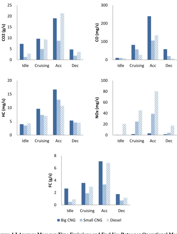
The average emissions and fuel use rates of each operational mode of each bus type were calculated and plotted in histograms, in order to identify if operational mode had similar impacts on emissions and fuel use rates for the different bus types. The same analysis was made on mass per distance and mass per fuel used rates as well.

5. Assess the relative importance of each operational mode on emissions and fuel use rates

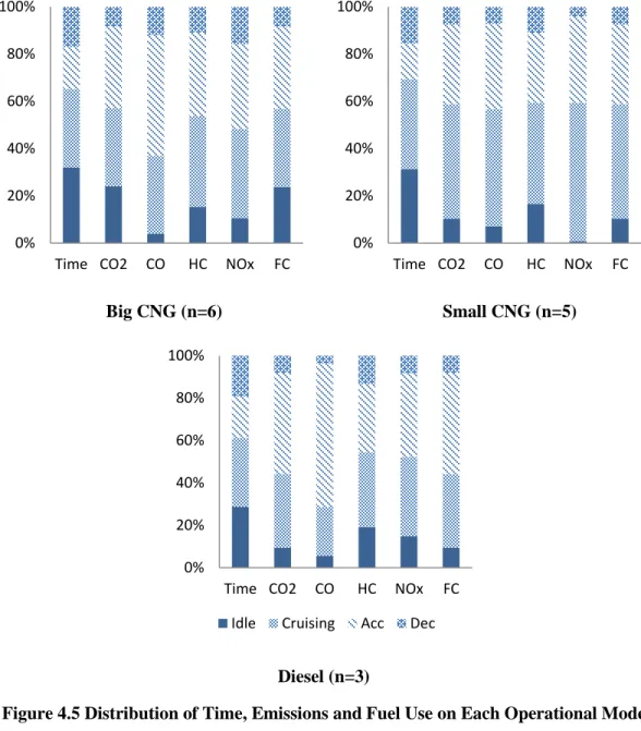
The percent of time, emissions and fuel use of each operation mode were calculated and compared with each other for each type of buses. The modes with less percent of time but more emissions and fuel use were identified as the ones with more relative importance on emissions and fuel use. The results of all types of buses were also compared to find if each operational mode has the same relative importance for each type of buses.

3.2.2.3.Engine Modal Comparison

This section discusses the methodology used to quantify the engine performance impacts on emissions and fuel use rates of all tested buses. Several tasks are conducted to develop this method.

1. Choose one engine parameter to identify the engine modes

Based on the dataset, several engine parameters were checked to identity engine variables that were highly correlated with emissions and fuel use rates. These variables included RPM, MAP (or MAF) and LOAD. Among these three parameters, RPM had the highest correlation values and lowest coefficient of variation values for most test buses. Furthermore, RPM may be read directly from the vehicle dashboard, which facilitates data collection. Thus, in this study, RPM was chosen as the indicator of engine modes.

(38)

29

2. Categorize the RPM into 10 engine modes for each tested bus

The dataset shows tested buses have various ranges of RPM values, especially among different types of buses. In order to compare the buses on a consistent basis with RPM values, the measured RPM values were normalized by the following equation:

𝑅𝑃𝑀𝑛𝑜𝑟 =

𝑅𝑃𝑀 − 𝑅𝑃𝑀_𝑚𝑖𝑛

𝑅𝑃𝑀_𝑚𝑎𝑥− 𝑅𝑃𝑀_𝑚𝑖𝑛 Equation 3

Where,

RPMnor = Normalized RPM for a measured RPM for a specific item of equipment

RPMmax = Maximum RPM for a specific item of equipment

RPMmin = Minimum RPM for a specific item of equipment

RPM = Measured RPM for a specific item of equipment

Considering the character of this equation, the overall normalized RPM values range from zero to one (or 0% to 100%). The normalized RPM values from minimum to maximum were further categorized into 10 individual bins, ranging from 0 to 0.1, 0.1 to 0.2…0.9 to 1.0. These 10 bins represent the 10 engine modes. For example, 0.0 to 0.1 refers to engine mode 1; and 0.1 to 0.2 refers to engine mode 2. Engine mode 1 typically represents the minimum load imposed on the engine, and engine mode 10 represents the maximum engine load.

3. Quantify the amount of time spent on each engine mode

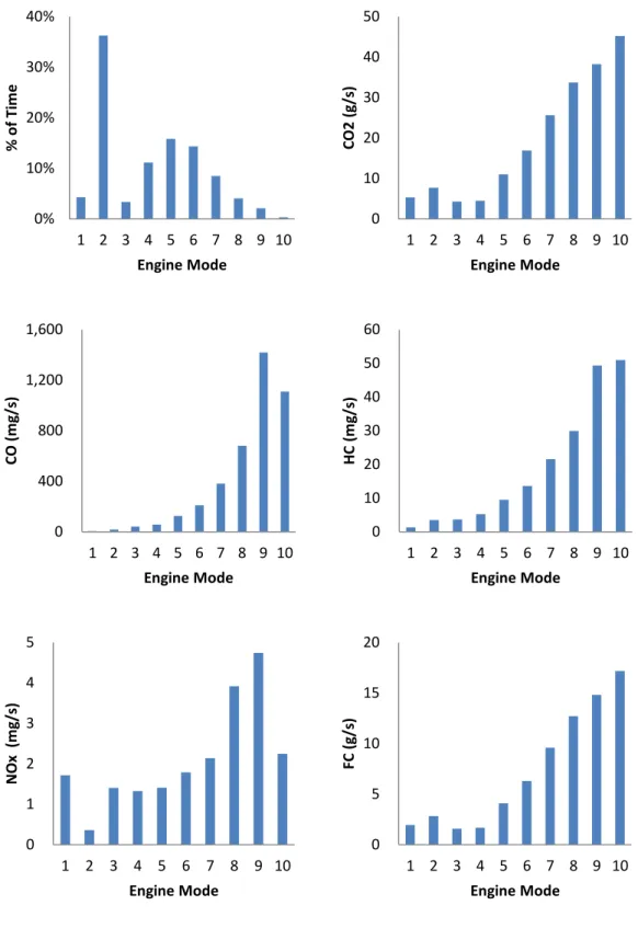
The amount of time spent on each engine mode for each tested bus was quantified. Based on that, the fraction of time spent on each engine mode was also calculated. Furthermore, in order to compare the time distribution among the three types of buses, the average percentage of time spent on each engine mode was calculated for each type of bus. Histograms were developed for time distribution among engine modes, which were used to demonstrate the relationships among the time spent on all engine modes of each type of buses.

(39)

30

4. Quantify the average emissions and fuel use rates for each engine mode

In order to demonstrate the relationships between the engine modes and emissions and fuel use rates, the average emissions and fuel use rates of all engine modes were calculated and

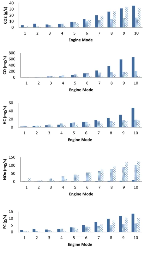
histograms were plotted for all tested buses. These histograms were also compared with the time histogram in order to find the relationship between emissions and fuel use rates, and time distribution among the ten engine modes. The overall average emissions and fuel use rates of each engine mode for each type of bus were also calculated and plotted, which were then used to compare the results among the three types of buses.

5. Calculate weighted average emissions and fuel use rates for each engine mode

For each tested bus, the weighted average emissions and fuel use rates of each engine mode were calculated by multiplying the percent of time and the average emissions and fuel use rates of that particular engine mode. The total weighted average emissions and fuel use rates of each bus were also calculated by the following equation:

𝑇𝑊 𝐸_𝑇 = ∑ 𝑇_𝑖× 𝐸_𝑇𝑖 10 𝑖=1 Equation 4 𝑇𝑊 𝐹𝑇 = ∑ 𝑇𝑖 × 𝐹𝑇𝑖 10 𝑖=1 Equation 5 Where,

TW ET= Total weighted average mass per time emission rates (g/s)

TW FT= Total weighted average mass per time fuel use rates (g/s)

Ti=Percent of time for ith engine mode, i=1, 2, 3…10

ETi=Mass per time emission rates for ith engine mode, i=1, 2, 3…10

(40)

31 3.3. Emissions and Fuel Use Predictive Models

In order to estimate emissions and fuel use rates based on engine performance, predictive models were developed for each pollutant and fuel use using engine performance data. The engine performance data included RPM, IAT, MAP (or MAF), LOAD, and SPEED. Two-third of the data for each tested bus was used as the training set, and the one-third of data was used for validation of the models. Multiple Linear Regression (MLR) was used to develop the predictive models.

3.3.1. Correlation Matrix

Correlations were used to assess the dependent relationships between emissions, fuel use and engine performance variables. There are several correlation coefficients to measure the degree of correlations. In this research, the Pearson correlation coefficient was used, which is considered to be the most common and sensitive only to a linear relationship between two variables. The Pearson correlation coefficient’s range is (-1 to +1). Positive one indicates a perfect increasing relationship and negative one indicates a perfect decreasing relationship. A correlation matrix is expressed by a table, which displays the coefficients of the columns and rows. In this study, emissions, fuel use and engine variables were included in the matrix in order to assess their relationship with each other.

3.3.2. Prediction Models using Multiple Linear Regression (MLR)

A Multiple Linear Regression model is a model that numerically describes the linear correlations between a single dependent variable and two or more independent variables. In this study, a model was developed for each of the four gaseous pollutants and fuel use, respectively based on the engine performance variables. The model is written in the form:

(41)

32

In this equation, Y is the dependent variable, which is the predictive value of each pollutant emission rate (or fuel use). The independent variables, Xi, i=1, 2…, m, are the engine

performance variables, such as MAP, RPM and IAT. β0 is the intercept, and β are the parameters for each independent variable. The βi, i=1, 2…, m, and β0 were estimated based on the dependent and independent variables data. The model development process was conducted using the

statistical software, SAS 9.3. The units of dependent and independent variables in the models was the original unit reported by PEMS, which are gram per second for CO2 and FC; milligram per second for CO, HC and NOx; revolution per minute for RPM; Celsius degree for IAT; kilo Pascal for MAP (or gram per second for MAF); percent (%) for LOAD, and kilometer per hour for SPEED.

The first step of model development was to examine if all the independent variables were necessary or a subset of them was adequate. In order to achieve this goal, the stepwise model selection method was applied which is a semi-automated procedure of building a model by adding or removing variables. This selection process started with no independent variables in the model, tested the addition of each variable, added the variable that improved the model the most, and repeated this process until none improved the model. If the variables that had been included in the beginning were no longer significant, those variables would be eliminated in the model. The p-value of each independent variable was checked to determine if this variable should be included in the model. If p-value of was less than 0.05, the variable was significant of the model; in other words, the variable should be included in the model. Conversely, if p-value was greater than 0.05, the variable should be excluded from the model.

After the stepwise model selection, an important statistics of the MLR model was checked for each independent variable, which is the Variance Inflation Factor (VIF). VIF was used to quantify the severity of multicollinearity in the MLR model. When multicollinearity occurs in the MLR model, it means two or more independent variables are highly correlated. Although it does not

(42)

33

reduce the predictive power and accuracy of the model, it may make the model more complicated and cumbersome. A VIF of 5 or above indicates a multicollinearity problem. In this study, an independent variable that was bigger than VIF=5 would be excluded. The model would be adjusted until all the VIF values of independent variables were smaller than 5.

After model development, SAS 9.3 provided several statistics to assess the appropriateness of the model, such as root of mean square error (Root MSE) and R-square. Root MSE is the square root of the mean square error of the models, and lower Root MSE values indicate there are fewer errors in the models. R-square refers to coefficient of determination, which is a measurement of the effect of the independent variables in reducing the variation in dependent variable. It ranges from zero to positive one (or 0% to 100%). Zero (or 0%) indicates that the model explains none of the variability of the response data, and positive one (or 100%) indicates that the model explains all the variability of the response data. In this study, R-square was used to evaluate the appropriateness of the multiple linear regression models.

3.3.3. Model Validation

Model validation was used to determine how well the results from the predicted models fitted the actual data. After the predictive models were developed based on the two-third of total data for the tested bus, they were used to predict the emissions and fuel use rates of the remaining one-third data; then, simple linear regression analysis was conducted between the actual values and the predicted values of the remaining one-third data by Excel 2010. Simple linear regression is a method to describe the linear relationship between two variables. The software provided the equation in the following form. The R-squarevalue of this equation was also estimated by Excel 2010.

(43)

34

In equation 7, m was a parameter to assess the accuracy of the predictive model; the closer it was to 1, the accuracy was higher. The parameter b was used to assess the bias of the predictive model. A higher b value showed a greater bias. The R-square was used to assess the precision of the predictive model. Its range was from zero to positive one (0% or 100%). Positive one (or 100%) indicated 100% precision, and zero (or 0%) indicated 0% precision. Model validation was conducted for all MLR predictive models.

3.3.4. Variable Impact Analysis

A statistics method was developed to assess the impacts of each engine variable on MLR models of each type of buses. The stepwise selection has already made for each model of each tested bus in model development section. The order number of each variable of each model was filled in the variable impact table for Big CNG, Small CNG, and Diesel buses, respectively. There were several models excluding some engine variables because either the variables were not significant, or the variables led to multicollinearity problems. The order number of these excluding variables was six.

Then, the order numbers of each engine variable were summed for each type of buses. These summation values were the impact parameters, which stood for the impacts of the engine

variables in each type of buses. The smaller values of impact parameters indicated that the engine variables had more influences on the models.

3.4. Emissions Inventory

An emissions inventory itemizes the quantities of air pollutants emitted for a specific area, period, and set of sources. This section introduces a methodology developing the emission inventory for the current OSU CNG bus fleet and the old diesel bus fleet. The goal of this research is to assess the environmental impacts of the CNG bus fleet. There are two primary components of the emissions inventory: (1) annual fuel use; and (2) estimated annual emissions.

(44)

35 3.4.1. Annual Fuel Use

The OSU fleet owner provided a fuel use database of the old diesel bus fleet, which contains the number of gallons of diesel fuel consumed by, and the operational hours of, each diesel bus during 2009 to 2010. Based on this database, the annual fuel use (DGE/yr) and the annual operation hour (hr/yr) of the diesel bus fleet were calculated.

The fuel use data of the current CNG bus fleet was not provided. Since the transit system did not change the routes when switching from the diesel fleet to the CNG fleet, it is appropriate to assume that the annual operation hour of the fleet kept same these years. Thus, the annual operation hour of the CNG fleet were roughly estimated as the diesel fleet’s annual operation hour. Because there are nine Big CNG buses and 10 Small CNG buses, the annual operation hour of the Big CNG buses was estimated as the 9/19 of the total annual operation hour, and the annual operation hour of the Small CNG buses was estimated as the 10/19 of the total. Then, the annual fuel use (DGE/yr) of the Big CNG fleet and the Small CNG fleet were estimated as multiplying their annual operation hour (hr/yr) by their average fuel use rates (DGE/hr), respectively. The summation of the annual fuel use of the Big CNG fleet and the Small CNG fleet is the annual fuel use of the whole CNG fleet.

3.4.2. Estimated Annual Emissions

For the diesel fleet, the average emissions rates (g/DGE) of each bus were multiplied by its annual fuel use (DGE/yr), and then, the summation of the annual emissions of all diesel buses were the annual emissions of the diesel fleet. Since there were only three diesel buses were tested, the emissions rates of the other buses were estimated as the average emissions rates of the three tested buses.

For the CNG fleet, there were only estimated annual fuel uses of the Big CNG and Small CNG fleet. Thus, the annual emissions of the Big CNG fleet were roughly estimated as multiply the

(45)

36

average emissions rates (g/DGE) of the tested Big CNG buses by its annual fuel use (DGE/yr). The annual emissions of the Small CNG fleet were estimated by the same procedure. The summation of these two CNG fleets was the annual emissions of the whole CNG fleet.

(46)

37

CHAPTER V

RESULTS 4.

4.1. Characterization of OSU Bus Fleet Data

This section presents the characters of OSU bus fleet data, including field data collection, and emission rates and vehicle activity data.

4.1.1. Field Data Collection

Table 4.1 shows the summary of the field data collection effort. 11 of the field tests were completed in 2013 and three in 2014. The buses were tested on eight different routes including a variety of on- and off-campus routes. There were approximately 59,000 seconds (16 hours) of data collected for the Big CNG buses, approximately 39,000 seconds (11 hours) for the Small CNG buses, and approximately 32,000 seconds (9 hours) for the diesel buses; thus, the overall data collection effort yielded over 36 hours of usable data on a second-by-second basis. Although the information was not used for this research project, the research team recorded the ambient temperature and humidity at the time of the test. The bus number was used to represent tested

(47)

38

buses in the result chapter. Big CNG 1568 bus was tested two times on two different routes. The two tests were numbered as Bus 1 and Bus 2, so that the data of both tests could be analyzed.

Table 4.1 Data Collection Summary Bus

Type Bus

No.

Bus

ID Date Route Data (s)

Ambient Conditions T (℃) H (%) Big CNG 1 1568 03.19.2013 Gray 9831 3 61 2 1568 09.11.2013 Orange 5926 30 43 3 1572 09.19.2013 Gray 11855 22 78 4 1566 09.20.2013 Scarlet 9560 18 77 5 1567 09.27.2013 White 10047 28 54 6 1569 11.08.2013 Orange 11544 7 76 Small CNG 7 1555 03.21.2013 Gray 10001 3 40 8 1556 09.13.2013 Blue 8923 24 60 9 1560 10.08.2013 Black 7315 6 92 10 1561 12.20.2013 Purple 6582 5 56 11 1558 06.12.2014 Blue 6319 20 82 Diesel 12 1530 03.20.2013 Gray 13256 -2 40 13 1544 07.10.2014 Brown 9234 23 73 14 1532 07.16.2014 Gray 9232 18 81

4.1.2. Emissions Rates and Vehicle Activity Data

Typical statistics values were calculated for each variable of engine performance data (RPM, IAT, MAP, LOAD and SPEED), emissions data (CO2, CO, HC and NOx ), and fuel consumption data (FC). These statistics included maximum, minimum, mean, standard deviation, and coefficient of variation. Table 4.2, Table 4.3and Table 4.4 present the summary statistics for the Big CNG, Small CNG, and Diesel buses respectively. These tables include values for vehicle and engine activity data, emissions rates, and fuel consumption (FC) rates. Note that Table 4.2 and Table 4.4 provide MAP data and Table 4.3 provides mass air flow (MAF) data in lieu of MAP. MAP data was not available through the OBD system on the Small CNG buses but MAF data was available. Either MAP or MAF is required by the Axion RS+ to calculate the mass per time emissions rates based on pollutant concentrations in the exhaust flow from the tailpipe.

(48)

39

Fo

Characterization of pollutant emissions and fuel use for CNG transit buses