R E S E A R C H
Open Access
A POD-based reduced-order FD extrapolating
algorithm for traffic flow
Zhendong Luo
1*, Di Xie
1and Fei Teng
2*Correspondence:
[email protected] 1School of Mathematics and
Physics, North China Electric Power University, Bei Nong Road, Beijing, 102206, China
Full list of author information is available at the end of the article
Abstract
A traffic flow Lighthill, Whitham, and Richards (LWR) model is studied by means of a proper orthogonal decomposition (POD) technique. A POD-based reduced-order finite difference (FD) extrapolating algorithm (FDEA) with lower dimension and fully second-order accuracy is established. Two numerical experiments are used to show that the POD reduced-order FDEA is feasible and efficient for finding numerical solutions of traffic flow LWR model.
MSC: 76M20; 65M12; 65M15
Keywords: traffic flow LWR model; proper orthogonal decomposition;
reduced-order finite difference extrapolating algorithm; numerical simulation
1 Introduction
Traffic is the lifeblood of the national economy. Advanced transportation and manage-ment systems are important symbols of modernization for the nation. The study of traffic flow has become a significant research topic (see,e.g., [–]).
The mathematical model of the traffic flow is generally a nonlinear system of partial differential equations (PDEs). Due to its nonlinearity, there are no analytical solutions in general. One has to rely on numerical solutions. The classical finite difference (FD) scheme (FDS) is one of the most effective numerical methods to solve the nonlinear system of PDEs for the traffic flow. However, the classical FDS usually includes a great number of degrees of freedom (namely, unknown quantities) so as to cause a lot of truncation error accumulation in computational process. Thus, even a very good FDS may appear to show no convergence after some computing steps. Therefore, an extremely meaningful problem is how to establish a reduced-order FDS with fewer degrees of freedom and sufficiently high accuracy.
The proper orthogonal decomposition (POD) method (see [–]) is an effective means to reduce the degrees of freedom of numerical models for time-dependent PDEs and alle-viate load calculating and the accumulation of truncation errors in the computational pro-cess. It is mainly to find an orthonormal basis for the known data under the least squares sense, namely, it is to find optimal order approximations for the known data. By using the POD technique, some POD reduced-order FDSs and finite element formulations for time-dependent PDEs have been established (see,e.g., [–]).
Though an extrapolation reduced-order FDS based on POD technique for the traf-fic flow Aw-Rascle-Zhang (ARZ) model has been presented (see []), it has only
order time accuracy. To the best of our knowledge, there is no report that the POD-method is used to reduce the degrees of freedom of the FDS for the traffic flow Lighthill, Whitham, and Richards (LWR) model (see [, ]). Especially, most of the existing POD-based reduced-order numerical computational methods (see,e.g., [–, , –, , ]) employ the numerical solutions obtained from classical numerical methods on the to-tal time span [,T] to construct POD bases and POD-based reduced-order models, and they then recompute the solutions on the same time span [,T], which actually belong to repeating computations on the same time span [,T]. The method in this paper aims to use only the first few given classical FDS solutions to construct the POD basis and to establish a POD-based reduced-order FD extrapolating algorithm (FDEA) with fully second-order accuracy and very few degrees of freedom for the traffic flow LWR model. It is equivalent to making use of very few given data to infer the future traffic status, which is a very meaningful work. Though a POD-based reduced-order FDEA for the non-stationary Navier-Stokes equations has been established in [], it has only first-order time accuracy too. Moreover, a POD-based reduced-order FDEA with fully second-order accuracy for a non-stationary Burgers equation has been posed in [], but the LWR model here is differ-ent from the non-stationary Burgers equation. Therefore, the POD-based reduced-order FDEA with fully second-order accuracy here is a new method and an improvement for the existing POD-based reduced-order numerical methods (see,e.g., [–]).
The paper is organized as follows. Section recalls the classical Lax-Wendroff scheme (LWS) (see [–]) for the traffic flow LWR model and generates snapshots from the first few numerical solutions computed from the equation system derived by the classical LWS. In Section , the optimal orthonormal POD basis is reconstructed from the elements of the snapshots via a singular value decomposition (SVD) technique and POD-method, and then the POD-based reduced-order FDEA with very few degrees of freedom and fully second-order accuracy for the traffic flow LWR model is established. In Section , the er-ror estimates of the POD-based reduced-order FDEA solutions and the implementation for the POD-based reduced-order FDEA are provided. In Section , two numerical exper-iments are used to validate the feasibility and efficiency of the POD-based reduced-order FDEA. Section provides main conclusions and discussions.
2 Recall LWS for the traffic flow LWR model
The traffic flow LWR model is denoted by the following Euler conservation PDE defined on [,J]×[,T]:
⎧ ⎪ ⎨ ⎪ ⎩
∂ρ ∂t +
∂q
∂x= , (x,t)∈(,J)×(,T),
ρ(x, ) =ρ(x), x∈(,J),
ρ(x,t) =ρ(x,t), x= ,J,t∈(,T),
()
whereρ∈(,ρm) is the density,ρm the maximum (jam) density,q(ρ) the traffic flow on a homogeneous highway, which is assumed to be only a function of the densityρin the LWR model,ρ(x) the given initial density, and ρ
(x,t) the given density on boundary. More specifically, the flowq, the densityρ, and the equilibrium speeduare, respectively, related by
q=um
– ρ
ρm
ρ, u=um
– ρ
ρm
whereumis the maximum limited speed. Thus, the traffic flow LWR model for the density the local truncation error of the fully second-order accuracy (see [, ]), namely we have the following error estimates:
ρ(xi,tn) –ρin=O x,t
, ≤n≤N, ≤i≤I. ()
Further, we can, respectively, obtain the approximate solutions of the flowqand the equi-librium speedufrom () as follows:
qni =um
which have also the local truncation error of the fully second-order accuracy, namely we have the following error estimates:
q(xi,tn) –qni+u(xi,tn) –uni=O x,t
, ≤n≤N, ≤i≤I. ()
For given time-step incrementt, spatial step incrementx, maximum (jam) density
ρm, maximum limited speedum, initial densityρ(x), and densityρ(x,t) on the boundary, by solving the FDS (), we can obtain the classical FD solutionsρn
i (≤n≤N, ≤i≤I) of the density for the traffic flow LWR model. Further, we also obtain the classical FD solutionsqn
i anduni (≤n≤N, ≤i≤I) of the flowqand the equilibrium speedufor the traffic flow LWR model from (). We may choose the firstLsolutions to construct a set{ρil}Ll=(≤i≤I,LN) withL×melements from the set{ρin}Nn=(≤i≤I) of the classical FD solutions of density withN×Ielements, which are known as snapshots.
3 Form POD basis and establish POD-based reduced-order FDEA
3.1 Form POD basis for snapshots increasing order. They are connected to the eigenvalues of the matricesAATandATAin a manner such thatλi=σi(i= , . . . ,) andλ≥λ≥ · · · ≥λ.
Since the number of spatial nodes is far larger than that of time nodes extracted,i.e.,
IL, namely the orderIfor matrixAAT is far larger than the orderLfor matrixATA, however, their non-zero eigenvalues are identical. Thus, we may first find the eigenvalues
λjand the orthonormal eigenvectorsϕj(j= , , . . . ,) corresponding to the matrixATA, and then by the relationship
φj=
σj
Aϕj, j= , , . . . ,, ()
we may obtain the orthonormal eigenvectorsφj(≤j≤≤L) corresponding to the non-zero eigenvalues for matrixAAT.
Let the norm of a vector). According to the relationship properties of the spectral radius and
· ,for the matrix, ifM<=rankA(≤L), we have It is shown thatAMis an optimal representation ofAand its error is
√
λM+. Denote theLcolumn vectors of matrixAbyal= (ρl
,ρl, . . . ,ρml )T (l= , , . . . ,L) andεl (l= , , . . . ,L) by unit column vectors except that thelth component is , while the other components are . Then we have
where alM=Mj=(φj,al)φj, (φj,al) is the canonical inner product for vectors φj andal. Inequality () shows thatal
Mare the optimal approximation toaland their errors are all
√
λM+. Then= (φ,φ, . . . ,φM) (ML) is an orthonormal basis corresponding toA, which is known as an orthonormal POD basis.
3.2 Establish the POD-based reduced-order FDEA for the traffic flow LWR model
In order to establish the POD-based reduced-order FDEA for the traffic flow LWR model, it is necessary to introduce the following symbols:
ρIn= ρn,ρn, . . . ,ρInT, αIn= αn,αn, . . . ,αMnT,
ρI∗n= ρ∗n,ρ∗n, . . . ,ρI∗nT=αnI,
()
and to rewrite () as the following iterative scheme:
⎧
Thus, the first equation of () is rewritten as the following iterative scheme of vector form:
ρnI+=ρnI +Q ρInρnI, ≤n≤N– , ()
whereQ(ρn
I) is a matrix determined by the second and third terms on the right hand of the first equation in (). reduced-order FDEA which only contains M degrees of freedom on every time level (n>L): columns inare orthonormal vectors, the second equation in () multiplied byTis reduced into the following POD-based reduced-order FDEA:
FDEA solutions for the traffic flow LWR model are presented as follows:
Further, we can obtain the POD-based reduced-order FDEA solutions of the flowqand the equilibrium speeduas follows, respectively:
q∗in=um
Remark . The system of equations () or () has no repeating computation and is
different from the existing POD-based reduced-order numerical computational methods (see,e.g., [–, –]) based on POD technique.
4 Error estimates of solutions and implementation for the POD-based reduced-order FDEA
In this section, we devote our efforts to deriving the error estimates of solutions for the POD-based reduced-order FDEA and the criterion of renewing POD basis and providing the implementation for the POD-based reduced-order FDEA.
4.1 Error estimates of solutions for the POD-based reduced-order FDEA
It is obvious that the second equation in () has also the following form like ():
ρi∗n+=ρi∗n+tum second equation in () has the following form like ():
ρ∗In+=ρ∗In+Q ρI∗nρ∗In, n=L,L+ , . . . ,N– . ()
Puten=ρn
I –ρ∗In. It follows from () that
en=ρnI –ρ∗In=ρnI –TρnI≤λM+, n= , , . . . ,L. ()
Under the stability condition, with ()-(), (), and (), we have
en+
Combining () with () yields the following results.
Theorem . Under the stability conditiont≤x/(um| –ρm|),we have the following
error estimates between the classical FDS solutions for the traffic flow LWR model and the solutions of the POD-based reduced-order FDEA()and():
ρnI –ρ∗In≤Cn(δ)λM+, ≤n≤N, ()
Since the absolute value of each component for a vector is not more than its norm, combining () with () yields the following results.
Theorem . Under the hypotheses of Theorem.,we have the following error estimates
between the accuracy solution for the traffic flow LWR model and the solutions of the POD-based reduced-order FDEA()and():
ρ(xi,tn) –ρi∗n=O Cn(δ)
λM+,x,t
, ≤i≤I, ≤n≤N. ()
Further,we have the following error estimates between the accuracy of the flow q and the equilibrium speed u and the POD-based reduced-order FDEA solutions in():
q(xi,tn) –q∗in+u(xi,tn) –u∗in
=OCn(δ)λM+,x,t
, ≤i≤I, ≤n≤N.
Remark . Due to POD-based reduced-order and extrapolation for the classical FDS,
the errors of solutions for the POD-based reduced-order FDEA in Theorem . include factorsCn(δ)√λM+ (≤n≤N) more than those for the classical FDS, but the degrees of freedom for the POD-based reduced-order FDEA are far less than those for the clas-sical FDS so that the POD-based reduced-order FDEA can greatly lessen the trunca-tion error accumulatrunca-tion in the computatrunca-tional process, alleviate the calculating load, save time-consuming calculations, and improve the actual computational accuracy (see the example in Section ). In particular, the error estimates of solutions for the POD-based reduced-order FDEA give some suggestions for choosing number of POD basis, namely, as long as we takeMsuch that√λM+=O(t,x).Cn(δ) = ( +δ)n–Lin Theorem . there is a suggestion for renewing the POD basis, namely, ifCn(δ)√λM+>min(t,x) (L+ ≤n≤N), the old POD basis is substituted with the new POD basis regenerated from the new snapshots (ρ∗l,ρ∗l, . . . ,ρI∗l) (l=n–L,n–L– , . . . ,n– ).
4.2 Implementation for the POD-based reduced-order FDEA
The implementation for the POD-based reduced-order FDEA ()-() consists of the fol-lowing five steps.
Step . For given time-step incrementt, spatial step incrementx, maximum (jam) densityρm, maximum limited speedum, initial densityρ(x), and densityρ(x,t) on the boundary, solving the following classical FDS at the first fewerLsteps (as usual, we take
Step . For the error=max(t,x) needed, decide on the numberM(M≤) of POD bases such that√λM+≤, and construct POD bases = (φ,φ, . . . ,φM) (where φj=Aϕj/λj,j= , , . . . ,M).
Step . Solving the following POD-based reduced-order FDEA:
⎧ ⎪ ⎨ ⎪ ⎩
αnI =TρnI, n= , , . . . ,L,
αnI+=αnI +TQ(αnI)αnI, n=L,L+ , . . . ,N– , ρ∗n
I = (ρ∗n,ρ∗n, . . . ,ρI∗n)T=αnI, n= , , . . . ,N,
one obtains the POD-based reduced-order FDEA solution vectorsρ∗In= (ρ∗n,ρ∗n, . . . ,ρI∗n), further, one obtains the POD-based reduced-order FDEA solutionsq∗in=um( –ρ∗
n i ρm)ρ
∗n i
and u∗n
i =um( – ρi∗n
ρm) (i= , , . . . ,I, n= , , . . . ,N) of the flowq and the equilibrium speedu.
Step . Let δ =tum| –ρm|/x. If ( +δ)n–L
√
λM+ ≤ (L + ≤n ≤ N), then ρ∗n
I = (ρ∗n,ρ∗n, . . . ,ρI∗n) (n= , , . . . ,N) are just solutions satisfying accuracy needed. Else, namely, if ( +δ)n–L√λ
M+>(L+ ≤n≤N), put (ρl,ρl, . . . ,ρIl) = (ρ∗l,ρ∗l, . . . ,ρI∗l) (l=n–L,n–L– , . . . ,n– ), and return to Step .
5 Some numerical experiments
In this section, we present two numerical experiments for the traffic flow LWR model to validate the feasibility and efficiency of its POD-based reduced-order FDEA.
5.1 Example for traffic flow case 1
Let the total length of road be , m, the restricted maximum velocityum= m/s, the maximum (jam) density ρm = . veh/m (where veh/m denotes the mean number of vehicles on each meter), the spatial step increment x= m, time-step increment
t= /, h,ρ(x) = . veh/m,ρ(,t) = . veh/m,ρ(J,t) = . veh/m (which is equivalent to the case that there is a traffic signal in the end of the road for restricting traffic flow). Consider the traffic situation in total timeT= s. Thus, the number of spatial nodesI= ,, the number of total time nodesN= ,.
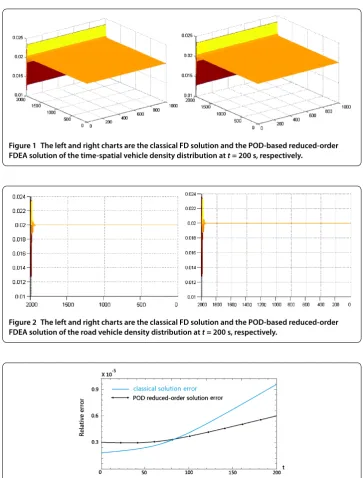
We find the numerical solutionsρin(≤i≤, and ≤n≤,) of the time-spatial vehicle density distribution and the numerical solutionsρin(≤i≤,,n= ,) of the road vehicle density distribution by means of the classical FDS (), depicted graphically on the left charts in Figures and , respectively.
Figure 1 The left and right charts are the classical FD solution and the POD-based reduced-order FDEA solution of the time-spatial vehicle density distribution att= 200 s, respectively.
Figure 2 The left and right charts are the classical FD solution and the POD-based reduced-order FDEA solution of the road vehicle density distribution att= 200 s, respectively.
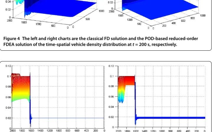
Figure 3 The relative errors of classical FDS solution and the POD-based reduced-order FDEA solution with seven POD bases on 0≤t≤200.
truncation error accumulation in the computational process, alleviate the calculating load, save time-consuming calculations, and improve actual computational accuracy, after some time span, the numerical errors of the POD-based reduced-order FDEA are fewer than those of the classical FDS (see Figure ). Thus, the POD reduced-order FDEA solutions are better and more stable than the classical FD solutions after a longer time.
5.2 Example for traffic flow case 2
time-Figure 4 The left and right charts are the classical FD solution and the POD-based reduced-order FDEA solution of the time-spatial vehicle density distribution att= 200 s, respectively.
Figure 5 The left and right charts are the classical FD solution and the POD-based reduced-order FDEA solution of the road vehicle density distribution att= 200 s, respectively.
step incrementt= /, h, but letρ(x) andρ
(x,t) be, respectively, as follows:
ρ(x) =
⎧ ⎪ ⎨ ⎪ ⎩
. veh/m, ≤x< ,, . veh/m, x= ,,
. veh/m, , <x≤,,
ρ(x,t) =
⎧ ⎪ ⎨ ⎪ ⎩
. veh/m, ≤t≤,x= ,
. veh/m, k– ≤t≤k,k= , , , , ,x= ,, . veh/m, k– ≤t≤k,k= , , , , ,x= ,.
This traffic situation is equivalent to the case that there is a traffic signal in the end of the road for restricting traffic flow. Total time is stillT = s. Thus, the number of spatial nodesI= ,, the number of total time nodesN= ,.
We find the numerical solutionsρin(≤i≤, and ≤n≤,) of the time-spatial vehicle density distribution and the numerical solutionsρin(≤i≤,,n= ,) of the road vehicle density distribution by means of the classical FDS (), depicted graphically on the left charts in Figures and , respectively.
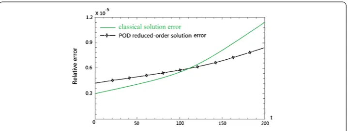
Figure 6 The relative errors of classical FDS solution and the POD-based reduced-order reduced-order FDEA solution with seven POD bases on 0≤t≤200.
Every two charts in Figures and also exhibit a quasi-identical similarity, respectively. Although the errors of the POD-based reduced-order FDEA solutions on starting time span are also slightly larger than those of the classical FDS solutions, since the POD-based reduced-order FDEA on each time level also includes only degrees of freedom and the classical FDS has more than , degrees of freedom, that is, the degrees of free-dom for the POD-based reduced-order FDEA are far fewer than those for classical FDS so that it could greatly lessen the truncation error accumulation in the computational pro-cess, alleviate the calculating load, save time-consuming calculations, and improve actual computational accuracy, after some time span, the numerical errors of the POD-based reduced-order FDEA are fewer than those of the classical FDS (see Figure ). Thus, the POD reduced-order FDEA solutions are better and more stable than the classical FD so-lutions after longer time.
6 Conclusions and discussions
In this paper, we have employed SVD-method and the POD-technique to generate the set of the POD basis and to establish the POD-based reduced-order FDEA for the traffic flow LWR model. We first compile ensembles of data from the first fewL(LN) transient solutions computing a system of equation derived with the classical FDS for the traffic flow LWR model, while in actual applications, one may obtain the ensemble of snapshots from real traffic flow by drawing samples. Next, we employ the SVD-method to deal with ensembles of data obtaining the POD basis. Then the classical FDS solution vectors are replaced with the linear combination of the most main POD basis to establish the POD-based reduced-order FDEA for the traffic flow LWR model. Finally, we provide the error estimates between the classical FD solutions and the POD-based reduced-order FDEA solutions and the implementation for solving the POD-based reduced-order FDEA of the traffic flow LWR model. Comparing the numerical computational results of the classi-cal FDS with these of the POD-based reduced-order FDEA shows that the POD-based reduced-order FDSEA is feasible and efficient for finding numerical solutions for the traf-fic flow LWR model. It is shown that our present method has improved and innovated the existing POD-based reduced-order methods (see,e.g., [–]).
If the POD-based reduced-order method is applied to more complicated traffic flow prob-lems and to establishing other nonlinear POD-based reduced-order schemes, that would be very interesting, which is a challenging and problem for our future studies. Future work in this area will aim to extend the FDEA, implementing it for a realistic and more compli-cated traffic flow forecast system.
Competing interests
The authors declare that they have no competing interests.
Authors’ contributions
All authors contributed equally and significantly in writing this article. All authors read and approved the final manuscript.
Author details
1School of Mathematics and Physics, North China Electric Power University, Bei Nong Road, Beijing, 102206, China. 2School of Mathematics Sciences, Kaili College, Kai Yuan Road 3#, Kaili, 24105, China.
Acknowledgements
This research was supported by National Science Foundation of China grant 11271127 and Science Research Project of Guizhou Province Education Department grant QJHKYZ[2013]207.
Received: 6 August 2014 Accepted: 2 October 2014 Published:14 Oct 2014
References
1. Aw, A, Rascle, M: Resurrection of second order models of traffic flow. SIAM J. Appl. Math.60, 916-938 (2000) 2. Lighthill, MH, Whitham, GB: On kinematics wave: II. A theory of traffic flow on long crowded roads. Proc. R. Soc. Lond.
A22, 317-345 (1955)
3. Mendez, AR, Velasco, RM: An alternative model in traffic flow equations. Transp. Res., Part B, Methodol.42, 782-797 (2008)
4. Richards, PI: Shock waves on the highway. Oper. Res.4(1), 42-51 (1956)
5. Siebel, F, Mauser, W: On the fundamental diagram of traffic flow. SIAM J. Appl. Math.66(4), 1150-1162 (2006) 6. Zhang, P, Wong, SC, Dai, SQ: A conserved higher-order anisotropic traffic flow model: description of equilibrium and
non-equilibrium flows. Transp. Res., Part B, Methodol.43, 562-574 (2009)
7. Zhang, P, Wong, SC: Essence of conservation forms in the traveling wave solutions of higher-order traffic flow models. Phys. Rev. E74(2), 026109 (2006)
8. Zhang, P, Liu, RX, Wong, SC, Dai, SQ: Hyperbolicity and kinematic waves of a class of multi-population partial differential equations. Eur. J. Appl. Math.17(2), 171-200 (2006)
9. Berkooz, G, Holmes, P, Lumley, JL: The proper orthogonal decomposition in analysis of turbulent flows. Annu. Rev. Fluid Mech.25, 539-575 (1993)
10. Holmes, P, Lumley, JL, Berkooz, G: Turbulence, Coherent Structures, Dynamical Systems and Symmetry. Cambridge University Press, Cambridge (1996)
11. Fukunaga, K: Introduction to Statistical Recognition. Academic Press, New York (1990) 12. Jolliffe, IT: Principal Component Analysis. Springer, Berlin (2002)
13. Sirovich, L: Turbulence and the dynamics of coherent structures: Part I-III. Q. Appl. Math.45, 561-590 (1987) 14. Di, ZH, Luo, ZD, Xie, ZH, Wang, AW, Navon, IM: An optimizing implicit difference scheme based on proper orthogonal
decomposition for the two-dimensional unsaturated soil water flow equation. Int. J. Numer. Methods Fluids68, 1324-1340 (2012)
15. Du, J, Zhu, J, Luo, ZD, Navon, IM: An optimizing finite difference scheme based on proper orthogonal decomposition for CVD equations. Int. J. Numer. Methods Biomed. Eng.27(1), 78-94 (2011)
16. Kunisch, K, Volkwein, S: Galerkin proper orthogonal decomposition methods for parabolic problems. Numer. Math.
90, 117-148 (2001)
17. Kunisch, K, Volkwein, S: Galerkin proper orthogonal decomposition methods for a general equation in fluid dynamics. SIAM J. Numer. Anal.40, 492-515 (2002)
18. Luo, ZD, Chen, J, Xie, ZH, An, J, Sun, P: A reduced second-order time accurate finite element formulation based on POD for parabolic equations. Sci. Sin., Math.41(5), 447-460 (2011) (in Chinese)
19. Luo, ZD, Chen, J, Zhu, J, Wang, RW, Navon, IM: An optimizing reduced order FDS for the tropical Pacific Ocean reduced gravity model. Int. J. Numer. Methods Fluids55(2), 143-161 (2007)
20. Luo, ZD, Du, J, Xie, ZH, Guo, Y: A reduced stabilized mixed finite element formulation based on proper orthogonal decomposition for the no-stationary Navier-Stokes equations. Int. J. Numer. Methods Eng.88(1), 31-46 (2011) 21. Luo, ZD, Gao, JQ, Sun, P, An, J: An extrapolation reduced-order FDS based on POD technique for traffic flow model.
Math. Numer. Sin.35(2), 159-170 (2013)
22. Luo, ZD, Li, H, Shang, YQ, Fang, ZC: A reduced-order LSMFE formulation based on proper orthogonal decomposition for parabolic equations. Finite Elem. Anal. Des.60, 1-12 (2012)
23. Luo, ZD, Li, H, Sun, P, Gao, JQ: A reduced-order finite difference extrapolation algorithm based on POD technique for the non-stationary Navier-Stokes equations. Appl. Math. Model.37(7), 5464-5473 (2013)
24. Luo, ZD, Li, H, Zhou, YJ, Xie, ZH: A reduced finite element formulation and error estimates based on POD method for two-dimensional solute transport problems. J. Math. Anal. Appl.385, 371-383 (2012)
26. Luo, ZD, Wang, RW, Zhu, J: Finite difference scheme based on proper orthogonal decomposition for the non-stationary Navier-Stokes equations. Sci. Sin., Math.50(8), 1186-1196 (2007)
27. Luo, ZD, Yang, XZ, Zhou, YJ: A reduced finite difference scheme based on singular value decomposition and proper orthogonal decomposition for Burgers equation. J. Comput. Appl. Math.229(1), 97-107 (2009)
28. Ly, HV, Tran, HT: Proper orthogonal decomposition for flow calculations and optimal control in a horizontal CVD reactor. Q. Appl. Math.60, 631-656 (2002)
29. Sun, P, Li, H, Teng, F, Luo, ZD: A reduced-order extrapolating algorithm of fully second-order finite difference scheme for non-stationary Burgers equation. Sci. Sin., Math.42(12), 1171-1183 (2012)
30. Sun, P, Luo, ZD, Zhou, YJ: Some reduced finite difference schemes based on a proper orthogonal decomposition technique for parabolic equations. Appl. Numer. Math.60(1/2), 154-164 (2010)
31. Sun, P, Luo, ZD, Zhou, YJ: A finite difference schemes based on POD for the non-stationary conduction-convection equations. Math. Numer. Sin.31(3), 323-334 (2009)
32. Chung, T: Computational Fluid Dynamics. Cambridge University Press, Cambridge (2002)
33. Liu, RX, Shu, QW: Several New Methods for Computational Fluid Mechanics. Science Press, Beijing (2003) (in Chinese) 34. Liu, RX, Wang, ZF: Numerical Simulation Methods and Motion Trace. University of Science and Technology of China
Press, Hefei (2001) (in Chinese)
10.1186/1687-1847-2014-269