Openness and inflation

Staff

PAPERS

FEDERAL RESERVE BANK OF DALLAS

No. 2

April 2007

Openness and Inflation

Mark A. Wynne and Erasmus K. Kersting

Staff

PAPERS

Staff

PAPERS

Federal Reserve Bank of Dallas

Openness and Inflation

Mark A. Wynne

Vice President and Senior Economist Federal Reserve Bank of Dallas

and

Erasmus K. Kersting

Ph.D. Candidate Department of Economics

Texas A&M University

Abstract

This paper reviews the evidence on the relationship between openness and inflation. There is a robust negative relationship across countries, first documented by Romer (1993), between a country’s openness to trade and its long-run inflation rate. However, a key part of the standard explana-tion for this relaexplana-tionship—that central banks have a smaller incentive to engineer surprise inflations in more-open economies because the Phillips curve is steeper—seems at odds with the facts. While the United States is still not a very open economy by conventional measures, there are chan-nels through which global developments may influence the nation’s infla-tion. We document evidence that global resource utilization may play a role in U.S. inflation and suggest avenues for future research.

JEL code: F4

Keywords: Openness, inflation, globalization, monetary policy

We thank Nathan Balke, Jian Wang, and participants in the Dallas Fed’s Brown Bag seminar for detailed comments on an earlier draft and Genevieve Solomon for her usual outstanding research assistance.

Staff

PAPERS

Federal Reserve Bank of Dallas

O

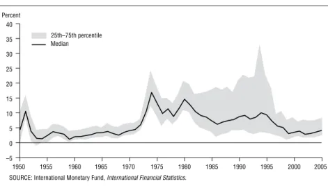
remarkable decline in inflation around the world. Figure 1 presents the basic facts. The median global inflation rate was 10 to 15 percent for most of the 1970s, 5 to 10 percent in the 1980s, and since then has been

around 5 percent or less.1 _{During the 1980s, the average annual inflation}

rate for developing countries was 36.7 percent and for industrial countries,

6.2 percent.2 _{In the 1990s, the numbers were 36 and 2.8 percent,}

respec-tively. Since 2000, inflation has averaged just 5.8 percent in developing

countries and 2 percent in industrial countries.3

Figure 1: Postwar Inflation Around the World

–5 0 5 10 15 20 25 30 35 40 2005 2000 1995 1990 1985 1980 1975 1970 1965 1960 1955 1950 25th–75th percentile Median

SOURCE: International Monetary Fund, International Financial Statistics. Percent

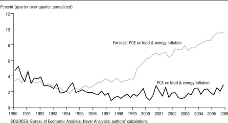
U.S. inflation has also dropped dramatically since the 1970s. After peaking at 11.5 percent in March 1980, inflation as measured by the Per-sonal Consumption Expenditures (PCE) deflator fell to an average of 4 to 5 percent by the latter half of the 1980s, then to 2 percent or less by the turn of the century. The low inflation the United States experienced in the late 1990s was unexpected. For most of the decade, inflation and un-employment declined together, contrary to what might be expected based on traditional Phillips curves, which posit a negative relationship between the two. This caused traditional models to systematically overestimate inflation, which gave rise to “missing inflation.”

Figure 2 shows the discrepancy between the actual inflation rate and a forecast series based on a traditional backward-looking Phillips curve model that includes lagged inflation, the U.S. unemployment rate,

1 _{We plot the median rather than the average inflation rate because of the existence of}

some extreme outliers.

2 _{We use the International Monetary Fund’s World Economic Outlook classification of}

countries as developing and industrialized.

3 _{The volatility and persistence of inflation also seem to have declined in recent years.}

Staff

PAPERS

Federal Reserve Bank of Dallas

and measures to control for aggregate shocks.4 _{A simple}

backward-look-ing Phillips curve estimated on data through fourth quarter 1990 does a reasonable job of forecasting inflation for the first couple of years of the decade but after 1995 or so, fails disastrously.

Figure 2: Missing Inflation of the 1990s

0 2 4 6 8 10 12 2006 2005 2004 2003 2002 2001 2000 1999 1998 1997 1996 1995 1994 1993 1992 1991 1990

Forecast PCE ex food & energy inflation

PCE ex food & energy inflation

Percent (quarter-over-quarter, annualized)

SOURCES: Bureau of Economic Analysis; Haver Analytics; authors’ calculations.

Many factors are believed to have contributed to the drop in inflation worldwide and in the U.S.: globalization, better monetary policy, luck, the emergence of the New Economy and the attendant acceleration of productivity, among them. All these factors likely played a role, and

disen-tangling the relative importance of each remains an important challenge.5

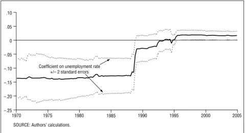
However, not only did inflation fall, there were also significant changes in the relationship between inflation and measures that have traditionally helped forecast inflation, as well as in inflation dynamics. It is now well es-tablished that U.S. inflation is less responsive to measures of the domestic output gap than in the past. Roberts (2006) is representative of the papers that have documented this.

Figure 3 shows recursive estimates of the coefficient on the unemploy-ment rate in the simple backward-looking Phillips curve model we use to generate the forecasts in Figure 2. The coefficient goes from being nega-tive and statistically significant for most of the 1970s and ’80s, to being marginally significant in the early 1990s, to having the wrong sign from

4 _{Specifically, inflation as measured by the annualized quarter-to-quarter change in the}

deflator for Personal Consumption Expenditures excluding food and energy is modeled as a linear function of four lags of itself (with the coefficients constrained to sum to 1), the lagged unemployment rate, and one lag of the quarter-to-quarter change in the price of oil imports relative to the GDP deflator.

5 _{For example, Ahmed, Levin, and Wilson (2004) look at the reasons for the markedly}

lower volatility in U.S. GDP growth and inflation since 1984 relative to the previous twenty-five years. They find that good luck (favorable exogenous circumstances independent of policy) is primarily responsible for the reduction in output volatility, while inflation has become more stable mainly due to good policy.

Staff

PAPERS

Federal Reserve Bank of Dallas

Figure 3: Recursive Estimates of the Coefficient on the Unemployment Rate in Simple Backward-Looking Phillips Curve

–.25 –.20 –.15 –.10 –.05 0 .05 .10 2005 2000 1995 1990 1985 1980 1975 1970

Coefficient on unemployment rate +/– 2 standard errors

SOURCE: Authors’ calculations.

the mid-1990s on. This particular pattern is, of course, specific to this

model, but it is qualitatively similar to that found in other models.6

This paper looks at the role globalization may have had in lowering inflation and making it less responsive to measures of domestic resource utilization, such as the unemployment rate. We survey the literature on openness and inflation and illuminate the channels whereby openness may

lead to lower inflation.7 _{We first look at different approaches to measuring}

the openness of economies along various dimensions. Then we describe the channels through which globalization may lower inflation. We examine the evidence on the importance of the various channels and evaluate the robustness of the findings in the empirical literature.

1. QUANTITATIVE DIMENSIONS OF GLOBALIZATION

We begin by presenting data that illustrate how integrated the world has become in recent years. Perhaps the best approach to measuring an economy’s openness—the extent of its integration with the rest of the world—is to look for deviations between the prices of goods and services within the economy from those prevailing on world markets. This approach is rarely adopted because of data limitations. As Knetter and Slaughter (1999) note, it is very difficult to obtain comprehensive international data

on local prices of products with identical characteristics.The limited data

that are available do not point to strong conclusions about the evolu-tion of market integraevolu-tion in recent years. In the price data they look at, Knetter and Slaughter find evidence of greater integration between the countries of Europe—little surprise, given the European Union’s major ef-forts in recent years to foster a single market. The evidence for developing countries is more mixed, with some seeming to converge in relative prices,

6 _{See, for example, Roberts (2006) or even earlier, Tootell (1998).}

Staff

PAPERS

Federal Reserve Bank of Dallas

while others do not. The quantity data Knetter and Slaughter examine show stronger evidence of product market integration since 1970.

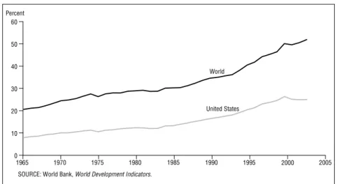
The most commonly used measure of openness is the sum of imports and exports divided by gross domestic product. Figure 4 shows the devel-opment of worldwide and U.S. openness over the past forty years. Imports and exports as a share of world GDP rose from 20 percent in 1965 to more than 50 percent in 2003. Over the same period, the importance of trade in goods and services to the U.S. economy rose from less than 10 percent to about a quarter of GDP.

Figure 4: Trade Relative to GDP

0 10 20 30 40 50 60 2005 2000 1995 1990 1985 1980 1975 1970 1965 World United States

SOURCE: World Bank, World Development Indicators. Percent

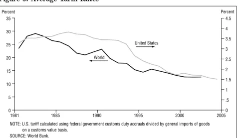
What has driven this increase in trade? Technological advances in transportation (most notably, the containerization revolution and devel-opment of larger ships and aircraft) and communication, as well as policy changes in the form of reduced tariff and nontariff barriers, have been key. Figure 5 presents some measures of average tariff rates for a variety of countries. There is a clear trend toward lower formal barriers to trade over the past four decades. Much of this has been driven by successive rounds of trade liberalization under the auspices of the World Trade Organiza-tion and its predecessor, the General Agreement on Tariffs and Trade. Of course, these data do not take account of the greater use of nontariff trade barriers in recent years.

Summarizing obstacles to free trade in a single measure is difficult, although Anderson and Neary (2005) have developed a framework that makes such calculations easier. Baier and Bergstrand (2001) assess the relative importance of income growth and changes in trade policy and transportation costs in the growth of trade between the countries in the Organization for Economic Cooperation and Development. They find that about two-thirds of the increase can be explained by income growth, with tariff rate reductions accounting for about a quarter and lower transporta-tion costs explaining just under 10 percent.

While these measures focus on trade in goods and services, an equally important dimension of openness relates to labor and capital flows. For

Staff

PAPERS

Federal Reserve Bank of Dallas

Figure 5: Average Tariff Rates

0 5 10 15 20 25 30 35 2005 2000 1995 1990 1985 1981 0 .5 1 1.5 2 2.5 3 3.5 4 4.5 United States World

NOTE: U.S. tariff calculated using federal government customs duty accruals divided by general imports of goods on a customs value basis.

SOURCE: World Bank.

Percent Percent

most of the postwar period, international capital flows were limited be-cause of widespread controls designed to facilitate the management of exchange rates under the Bretton Woods system. With Bretton Woods’ collapse in the early 1970s, capital accounts were gradually liberalized, and over time investors have become more willing to invest abroad. The International Monetary Fund (2006) reports that in the 1970s, more than three-quarters of industrial countries had restrictions of some sort on in-ternational financial transactions. By the 2000s, none did. Likewise, the percentage of emerging-market economies with restrictions on internation-al financiinternation-al transactions fell from 78.7 percent in the 1970s to 58 percent in the 2000s. As a result of these liberalizations, international capital flows have increased dramatically.

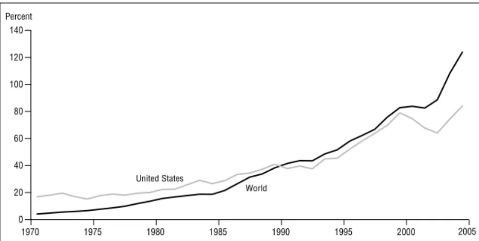
Figure 6 uses data from Lane and Milesi-Ferretti (2006) to give some sense of these capital flows’ importance. The figure shows the value of international (cross-border) assets plus liabilities held worldwide and by the United States as a percentage of GDP. This measure includes portfolio equity assets, foreign direct investment, and debt assets. International as-sets and liabilities as a share of global GDP rose from less than 5 percent in 1970 to more than 120 percent in 2004. For the U.S., foreign assets and liabilities amounted to just under 17 percent of GDP in 1970 but had risen to 84 percent by 2004.

While not as significant (quantitatively) as capital flows, flows of work-ers across national bordwork-ers are also an important dimension of globaliza-tion. We are accustomed to thinking of the United States as a nation of immigrants. As of 2005, immigrants accounted for 12.9 percent of the U.S. population (Figure 7). The U.S. also hosted 20 percent of all international migrants, by far the largest share of any country. Yet immigrants are also an important presence in other countries. They make up 12.3 percent of Germany’s population, 10.7 percent of France’s, 14 percent of Ireland’s, 20.3 percent of Australia’s, 62.1 percent of Kuwait’s, and 78.3 percent of Qatar’s. (In some cases, the large percentage of foreigners simply reflects the small size of the host country.)

Staff

PAPERS

Federal Reserve Bank of Dallas

Figure 6: Growth of International Capital Markets

0 20 40 60 80 100 120 140 2000 1995 1990 1985 1980 1975 1970 United States World 2005 SOURCE: Web appendix to Lane and Milesi-Ferretti (2006), www.imf.org/external/pubs/ft/wp/2006/data/wp0669.zip. Percent

Figure 7: International Migrants as a Percentage of the Population

0 2 4 6 8 10 12 14 2005 2000 1995 1990 1985 1980 1975 1970 1965 1960 World United States Percent

SOURCE: United Nations, Trends in Total Migrant Stock: The 2005 Revision.

At the global level, international migrants constitute only 2.9 percent of the world’s population, up from 2.1 percent in 1975. Much of the increase is the result of previously internal migrants being reclassified as interna-tional migrants after the Soviet Union’s disintegration in 1991. However, there have been dramatic changes in the international mobility of workers in the European Union, where formal barriers have been effectively elimi-nated. Countries like Ireland, the U.K., and Sweden—which immediately opened their doors to workers from the ten nations that joined the EU in 2004—have clearly benefited in recent years from increased immigration.

It is not just legal migration that matters for inflation. Passell (2006) estimates that about 7 million illegal immigrants work in the United States, accounting for just under 5 percent of the labor force. This is a nontrivial number and might be expected to have a noticeable effect on prices in the

Staff

PAPERS

Federal Reserve Bank of Dallas

sectors in which these immigrants work. Most are employed in sectors that produce services not traded internationally, such as construction, food service, and home maintenance. Assuming many of the immigrants in the United States illegally are low skilled, Cortes’ (2006) estimates suggest they may significantly affect the price of the average nontraded good.

Looking at the numbers, capital and goods are clearly more

interna-tionally mobile than workers.8_{Indeed, the presence of significant barriers}

to immigration is one of the key differences between the current era of globalization and the one that preceded World War I.

2. THEORY

Most traditional models have surprisingly little to say about globaliza-tion’s effect on price levels, as manifested in increased trade or factor flows. Rather, the emphasis has traditionally been on how economic integration (trade and factor mobility) affects relative prices and real factor returns. But we can obtain some insight into globalization’s potential effect on U.S. inflation by identifying some obvious channels. The direct and indirect price effects of cheaper imports of finished goods and intermediate inputs may net out to a decline in the overall price level. Additionally, opening an economy to the world may alter the incentives to which its central bank responds in determining the country’s long-run inflation rate.

For starters, there is a direct effect. Greater availability of cheaper goods from abroad will lower the domestic price level, since the consump-tion bundle used to compute broad inflaconsump-tion measures includes imported goods. The magnitude of this effect depends on the share of imports in the consumption bundle of the representative household. As countries become more open, the share of imports generally rises. But even in the most open economies, the consumption bundle includes a significant amount of nontraded goods and services. Perhaps the best example is the service flow from owner-occupied housing, which currently accounts for about a quarter of the U.S. Consumer Price Index. Furthermore, many goods traded internationally typically have to be combined with a large amount of nontraded domestic marketing and distribution services before they

reach the final consumer.9

Nevertheless, it is generally accepted that import prices may directly affect domestic price developments, and this has led to the inclusion of import prices in recent specifications of empirical Phillips curves. Inclusion of a measure of import prices (usually the prices of so-called core imports, which in the U.S. means imports excluding energy, computers, and semi-conductors) may also capture some of globalization’s indirect effects on the price level. For example, domestic producers are forced to lower their prices in response to foreign competition, and cheaper inputs from foreign

8 _{See Freeman (2006) for evidence; he notes a lot more variation in wages for similar}

occupations around the world than in prices of similar goods or in the cost of capital.

Staff

PAPERS

Federal Reserve Bank of Dallas

sources will lead to lower costs. The size of these effects will be governed by the ease with which foreign imports of intermediate and final goods can be substituted for domestically produced versions of the same goods. Yet another channel through which globalization may lower domestic prices is through lower nominal wage demands resulting from lower prices for im-ported final-consumption goods. Again, the size of this effect will depend on the importance of imports to the average worker.

Globalization could also lower inflation indirectly, with the increased competition fostering faster domestic productivity growth. Because trade enables countries to specialize in the activities in which they enjoy a com-parative advantage, sectors in which countries are relatively inefficient shrink, while sectors in which they have a comparative advantage expand. Faster productivity growth allows firms to pay higher wages without pass-ing these costs on in the form of higher prices.

Grossman and Helpman (1991) identify four possible channels through which increased openness might lead to faster productivity growth. First, increased trade between countries opens channels of communication that facilitate the transfer of technical knowledge. Second, greater openness increases the competitive pressure on firms to innovate. Third, with a larger market in which to sell, the rewards for successful innovation will be potentially greater. And fourth, the specialization brought about by economic integration may raise an economy’s growth rate if it prompts specialization in dynamic sectors.

In short, there are many ways in which increased openness can lead to a lower price level. However, it is important to keep in mind that most of these are one-time effects, implying a transitory impact on the inflation rate. Nevertheless, these one-time effects may take a long time to play out, implying that the temporary effect on the inflation rate may last quite a long time.

Furthermore, this discussion of effects is partial. A full examination of the ways increased integration might impact domestic inflation requires a fully articulated general-equilibrium model. The net effect of increased integration in such a model is less clear. For example, in the discussion above we mention that cheaper imports can directly affect the domestic price level. But this will be offset to some extent, depending on how house-holds make use of the resulting savings. If they spend all the gains on, say, domestically produced goods supplied inelastically, there will be an offset-ting inflationary effect on the domestic price level, which will partially or even completely offset the decline due to cheaper imports. Likewise, we need to take account of how the foreign suppliers use the proceeds from their export sales. With more countries participating in the global economy, there will be increased demand for scarce raw materials, which presumably will be reflected in their price, offsetting the price-level effects of cheaper imports.

Staff

PAPERS

Federal Reserve Bank of Dallas

10

Endogenous Monetary Policy

Examining the effects of increased openness while assuming no change in monetary policy gives us an incomplete picture of how globalization

might affect inflation. In the long run, central bank policies determine

inflation, and we need to consider how globalization might affect the infla-tion rate chosen by central banks over time. As Rogoff (2003) notes, the relative price effects associated with globalization will impact inflation only if the central bank chooses to let them.

The literature has advanced at least two lines of argument about how globalization might affect long-run inflation. The first, due to Rogoff (2003), considers the political economy of monetary policymaking under discretion that uses the workhorse model Barro and Gordon (1983) devel-oped. The gist of Rogoff’s argument is that by closing the gap between the

natural rate of output and the desired output level, globalization reduces

the inflation bias of central banks that are not constrained by rules. The second line of argument holds that in a more integrated world, competi-tion between currencies forces central banks to adopt best practices and keeps inflation low. This argument has been advanced by Wagner (2002), Tytell and Wei (2004), and others. Key to this “discipline effect” story is financial globalization, rather than real (goods and services) globaliza-tion.

The central idea in Barro and Gordon’s (1983) model, which is based on Kydland and Prescott’s (1977) insights, is that the monetary authority and the public are involved in a game, with the authority making decisions that influence the inflation rate and the public forming expectations ac-cordingly. The basic setup has proved useful in thinking about monetary policy and can help us understand the various hypotheses that have been advanced to explain the decline in global inflation in recent decades.

Assume that the central bank has the twin objectives of stabilizing

output, y, around some target level, y*, and inflation, π, around some

target level, π*. We can summarize these objectives in the quadratic loss

function

(1) L₌ ωy y y*_{− +}ωπ _{π π−}

2 ( )2 2 ( * ,)2

where w_y> 0 and w_π> 0 denote the weights the central bank assigns to its

output stabilization and inflation objectives. Let’s also assume output is determined by means of a standard Lucas supply function

(2) y =y_n+α(π-πe_)+ε,

where α> 0, y_n denotes the natural rate of output, πe _{denotes the expected}

rate of inflation, and εis a supply shock that has an average value of zero.

The parameter α determines the slope of the Phillips curve (specifically, it

is the inverse of the slope of the Phillips curve) and is not a deep structural parameter. Rather, in a more general model, it will depend on the degree of price flexibility in the economy and the conduct of monetary policy.

Staff

PAPERS

Federal Reserve Bank of Dallas

11

In this simple model economy, agents are assumed to form their infla-tion expectainfla-tions before they know whether the economy will experience a favorable or unfavorable supply shock. These expectations then feed into their decisions about wages and prices. Once the supply shock occurs, the central bank gets to decide monetary policy. For simplicity, we assume the central bank controls the inflation rate directly. When the central bank is not bound by a rule, it takes private-sector expectations of inflation as given when setting the inflation rate. Substituting the supply relation (equation 2) into the central bank’s objective function (equation 1) and choosing the level of inflation that minimizes the loss function, conditional on expected inflation, we obtain the central bank’s preferred inflation rate: (3) π ω α ωπ = +

}

{

ωyα(y*–yn)–ωyαε+ωyα2πe+ωππ* .

However, in a rational-expectations equilibrium, private-sector agents understand the incentives for the central bank to generate surprise infla-tions, and they will form their expectation of inflation accordingly. The equilibrium inflation rate each period, then, will be

(4) π π* α_ωω _{α ω α ω} ε π π = + y( − )− ₊ y 2 y* y_n ωy _,

while in the long run, when supply shocks average out to zero, inflation will be

(5) π π* α_ωω

π

= + y (_{y* y}− )

n .

The long-run equilibrium inflation rate consists of two terms. First,

the central bank’s target inflation rate, π*, and second, an inflation bias

term that arises due to the discretionary nature of the central bank’s decisionmaking. The size of the inflation bias depends on the output

effect of a surprise inflation (determined by α), the weight the central

bank puts on stabilizing output versus stabilizing inflation (as

reflect-ed in the ratio w_y/w_π), and the difference between the central bank’s

target level of output and the natural rate of output, y*– y_n.

Romer (1993) and Rogoff (2003) use this framework to illustrate how increased globalization might have permanent effects on inflation. Romer argues that more-open economies will have steeper Phillips curves and

thus lower values of α. The reason for this is that a monetary expansion

in an open economy will be accompanied by a real depreciation of the cur-rency, raising costs for households and businesses. The larger the share of imported goods, the greater the increase in inflation. Romer also argues that the relative weight on stabilizing output is smaller in more-open

Staff

PAPERS

Federal Reserve Bank of Dallas

1

economies, again because of the real depreciation induced by the monetary

shock.10

Rogoff argues that in a more competitive world—brought about by globalization, deregulation, and less government involvement in the econo-my—monetary policy has smaller effects on real activity, which means the Phillips curve is steeper and central banks have less incentive to inflate. Globalization also has permanent effects on the inflation rate by reducing the gap between the central bank’s target level of output and the natural rate of output:

…[M]onopoly in both the product and labor markets creates a wedge between the monopoly level of employment and the corresponding bench-mark competitive level. Such an imperfection provides the crucial moti-vation for the central bank to inflate in order to drive employment above its “natural” market determined rate. As the wedge becomes smaller,

there is less to gain from unanticipated inflation. Central bank anti-infla-tion credibility is enhanced, even without any instituanti-infla-tional change. As a consequence, average equilibrium inflation falls. Thus, an increased level

of competition in the economy—due either to globalization or deregula-tion—not only lowers the real prices of goods, but also tips coordination toward a lower inflation equilibrium. (Rogoff 2003, 65)

Before proceeding, we might note that if the central bank were able to commit to its target inflation rate, the inflation bias would disappear. And herein lies an important problem in figuring out what has caused inflation rates to fall. At the same time the world has become more integrated, we have seen an increased reliance on rules-based approaches to monetary policy, such as the widespread adoption of inflation targeting and greater

use of the Taylor rule.11 _{Both would lead us to expect inflation rates closer}

to the objectives of central banks. But the simple reduced-form framework sketched here does not allow us to distinguish the relative importance of each.

10 _{Lane (1997) points out that the terms-of-trade argument only applies to large countries,}

because the change in domestic output must be substantial enough relative to world output to change world relative prices. But the openness–inflation relationship holds empirically for small open countries as well. Consequently, Lane follows a different line of reasoning to explain the negative correlation. He constructs a two-sector model with a monopolistic nontraded goods sector and a competitive sector that produces the homogenous traded good. Unexpected inflation is beneficial in this setting because the monopolistic competition results in a lower output of nontraded goods than is optimal. Therefore, stimulating output in the short run can be welfare-improving. The effects of openness are straightforward: As the country becomes more open, the nontraded sector becomes less important than the traded goods sector. Therefore, the monetary authorities stand to gain less by creating surprise inflation in a more open economy.

11 _{Referring back to Figure 1, we see low, stable inflation rates in the 1950s and 1960s.}

One interpretation of the global inflation surge of the 1970s is that it resulted from the abandonment of the rules-based framework for monetary policy that existed under the Bretton Woods system of fixed exchange rates.

Staff

PAPERS

Federal Reserve Bank of Dallas

1 3. DOCUMENTING THE CORRELATION BETWEEN OPENNESS

AND INFLATION

We now move on to review some of the empirical studies of the rela-tionship between openness and inflation. Evidence suggests that greater openness is associated with lower trend inflation. Also, along many dimen-sions, the U.S. economy does not appear to be very open. Nevertheless, measures of global slack do seem more highly correlated with the cyclical component of U.S. inflation than are measures of U.S. slack.

Cross-Country Evidence

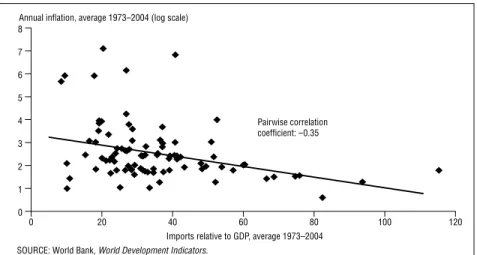
As noted above, Romer (1993) argues that a major implication of the literature on time consistency and monetary policy is that inflation should be lower in economies that are more open to trade. He documents a negative correlation between openness and long-run inflation, consistent with the theory. Figure 8 shows the basic relationship for a slightly smaller number of countries than Romer looks at, but for a longer period.

Figure 8: Inflation and Openness to Trade

0 20 40 60 80 100 120 0 1 2 3 4 5 6 7 8

SOURCE: World Bank, World Development Indicators.

Imports relative to GDP, average 1973–2004 Annual inflation, average 1973–2004 (log scale)

Pairwise correlation coefficient: –0.35

While Romer finds the basic correlation is robust to conditioning on other variables, he also finds essentially no relationship between openness and inflation for the most developed countries. Average inflation in the world’s richest countries tends to be low regardless of how open they are. Romer interprets this as suggesting these countries have largely solved the time-consistency problem that leads to higher inflation in less developed countries. However, subsequent research by Lane (1997) and Campillo and Miron (1997) finds that even for developed countries, greater openness is associated with lower inflation, after conditioning on additional variables. Lane emphasizes a different channel through which openness and inflation may be related: the degree of imperfect competition and price rigidity in the nontraded sector. Lane finds that by conditioning on additional vari-ables (country size, per capita income, and central bank independence), the relationship between openness and inflation is statistically significant (and negative) even for the advanced industrial nations. Campillo and

Staff

PAPERS

Federal Reserve Bank of Dallas

1

Miron also condition on a wider set of variables (measuring prior infla-tion experience, optimal tax considerainfla-tions, and time-consistency issues in areas other than monetary policy) and again find a statistically significant negative relationship between openness and inflation. This is made more

remarkable by the fact that the authors fail to find central bank

inde-pendence to be a substantial causal factor. Overall, Campillo and Miron

conclude that it is mainly structural factors—such as openness, political stability, and tax policy—not institutional arrangements that drive differ-ences in inflation across countries.

An obvious alternative to the widely adopted approach of using a cross-section specification to quantify the openness–inflation relationship is to make more use of the time-series structure of the data and use panel estimation methods. Alfaro (2005), Sachsida, Carneiro, and Loureiro (2003), and Gruben and McLeod (2004) take this approach. However, as Romer notes in his original contribution, “Investigating the time-series relationship between openness and inflation would be likely to yield biased estimates of the effects of openness.” The reason for this is that movement in openness within countries is caused by changes in trade policy and other macroeconomic factors that could also affect inflation—but through channels other than openness. Sachsida et al. and Gruben and McLeod use instrumental variable estimators to deal with the endogeneity problem, but Alfaro does not. The problem of cyclical movements in inflation can be mitigated by averaging observations over multiple years. For example, Gruben and McLeod partition the data into five-year averages. They and Sachsida et al. find that inflation decreases with openness, whereas Alfaro finds the opposite. However, based on our own examination of the data (not reported here), her finding seems to rest entirely on her use of an-nual data. Taking five-year averages, we again find a negative relationship between openness and inflation.

The literature that has grown out of Romer’s original contribution focuses on trade flows as the relevant dimension of openness restraining

inflation. The reason for this is the central role of the real exchange rate

depreciation in generating a steeper Phillips curve in more-open econo-mies, thereby creating a smaller incentive for central banks to inflate. But it is worth looking at some of the other dimensions of globalization to see whether they, too, are associated with lower long-run inflation rates. The two obvious additional dimensions to consider are openness to capital and labor flows.

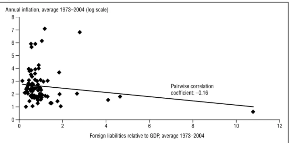
Figure 9 uses data from Lane and Milesi-Ferretti (2006) to plot each country’s average inflation rate over the past three decades against the average level of its foreign liabilities to its GDP. There is a negative corre-lation, but it does not appear as strong as that between long-run inflation

and openness to trade.12 _{The primary mechanism through which greater}

openness to foreign capital might lead to lower inflation is presumably some sort of disciplining effect on monetary policy, as Wagner (2002) and Tytell and Wei (2004) suggest.

12 _{Indeed, the negative correlation is driven by the outliers (Bahrain, Panama, and}

Hong Kong). Once these countries are dropped from the sample, there is a slight positive correlation between foreign liabilities relative to GDP and inflation.

Staff

PAPERS

Federal Reserve Bank of Dallas

1 Figure 9: Inflation and Openness to Capital Flows

Pairwise correlation coefficient: –0.16 0 2 4 6 8 10 12 0 1 2 3 4 5 6 7 8

Annual inflation, average 1973–2004 (log scale)

Foreign liabilities relative to GDP, average 1973–2004

SOURCES: World Bank, World Development Indicators; web appendix to Lane and Milesi-Ferretti (2006), www.imf.org/external/pubs/ft/wp/2006/data/wp0669.zip.

While much of the globalization literature focuses on the trade in goods and the movement of capital across borders, relatively little atten-tion has been paid to the effects of the movement of labor. This doubt-less reflects the barriers to international movement of workers. As noted above, while the United States has the most international migrants, for-eign workers constitute a larger share of other countries’ populations. The mechanism whereby openness to labor flows might lead to lower inflation is presumably by allowing the country to draw on a larger pool of

work-ers when economic activity is high.13 _{Inflows of foreign workers in boom}

times will restrain domestic wage pressures and lead to a flatter Phillips

curve.14

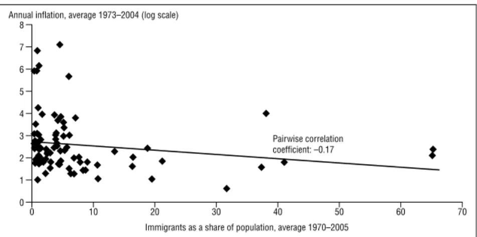
Figure 10 plots average long-run inflation against a crude measure of labor market openness, which is simply the share of the population that is foreign-born. Again, we see a weak negative correlation: Countries that are more open to labor flows seem to have lower inflation over the long run.

While considering each of these dimensions of openness in isolation is interesting, it would be useful to know how inflation correlates with some composite measure of openness. A number of such measures exist, among

13 _{Bank of England Governor Mervyn King has said it is likely the influx of workers to}

the U.K. from the countries that joined the EU in 2004 has helped restrain inflation pressures in the U.K. and enabled the central bank to keep interest rates lower than they would otherwise have been. In a June 2006 speech, King noted, “Over the past few years, the impact of migration, particularly from the new member countries of the European Union, has been substantial. The official data on total net migration are derived from small and incomplete surveys, so we cannot pretend to have an accurate idea of the real extent of migration. But, based on responses to the International Passenger Survey, net inward migration between 1995 and 2004 was estimated to have been 1.3 million, compared with a rise in the labor force as a whole of 1.7 million. We do know that the labour force has recently been expanding twice as fast as in the rest of the post-war period. Migration on this scale raised the potential growth rate of the UK economy and probably dampened the response of costs and prices to changes in demand” (King 2006).

14 _{Note that this is the exact opposite of the effect Romer and Rogoff emphasize,}

whereby inflation is lower in more-open economies because of a steeper Phillips curve, changing the monetary authority’s incentives.

Staff

PAPERS

Federal Reserve Bank of Dallas

1

them the A.T. Kearney/Foreign Policy Globalization Index and the index Andersen and Herbertsson (2003) developed. The A.T. Kearney index is a composite of measures of such factors as trade, telephone lines, tour-ism, and membership in international organizations. It covers sixty-two countries but is only available from 1999 on. A shortcoming of the index Andersen and Herbertsson note is that it does not control for country size and uses an arbitrary weighting scheme. They propose an alternative index that uses factor analysis to combine the various dimensions of open-ness in a single measure. While the Andersen and Herbertsson measure has a somewhat stronger statistical foundation than the A.T. Kearney index, it only covers twenty-three OECD countries.

Figure 10: Inflation and Openness to Labor Flows

0 10 20 30 40 50 60 70 0 1 2 3 4 5 6 7 8 Pairwise correlation coefficient: –0.17

SOURCES: World Bank, World Development Indicators; United Nations, World Migrant Stock: The 2005 Revision Population Database, http://esa.un.org/migration.

Annual inflation, average 1973–2004 (log scale)

Immigrants as a share of population, average 1970–2005

We instead focus on a subindex—the freedom to trade internation-ally—of the Fraser Institute’s Economic Freedom of the World index (Gwartney and Lawson 2006). This index is a composite measure of taxes on international trade, regulatory trade barriers, capital market restric-tions, and so on. It does not consider labor market openness. While this

measure does suffer from one of the samedisadvantages as the A.T.

Kear-ney measure (an arbitrary weighting scheme), it has the advantage of hav-ing a long time-series dimension, in addition to coverhav-ing every country in the world. Figure 11 plots each country’s average index score against its long-run inflation rate. Again, there is a noticeable negative correlation. Interestingly, the negative relationship between this measure of openness and long-run inflation seems to be a lot less dependent on extreme obser-vations.

The Sacrifice Ratio

As noted above, Romer identifies two key channels whereby greater

openness would lead to permanently lower inflation. The first isthe effect

of openness on the slope of the Phillips curve. The second is its effect on the weight assigned to output stabilization in the central bank’s objective

Staff

PAPERS

Federal Reserve Bank of Dallas

1 Figure 11: Inflation and Overall Openness

Pairwise correlation coefficient: –0.41 2 3 4 5 6 7 8 9 10 0 1 2 3 4 5 6 7 8

SOURCES: World Bank, World Development Indicators; Gwartney and Lawson (2006). Annual inflation, average 1973–2004 (log scale)

Freedom to trade internationally, average index value 1970–2000

function. It is difficult to measure the relative importance a central bank might assign to inflation versus output objectives and how that might cor-relate with globalization. It is easier to see if more-open economies have steeper or flatter Phillips curves.

Temple (2002) tests this key part of the Romer story by looking at whether Phillips curves are, in fact, steeper in more-open economies. He starts by examining the relationship between openness and the sacrifice ratios that Ball (1994) and Ball, Mankiw, and Romer (1989) compute for various disinflations. Temple finds that the relationship is at best weak and concludes the time-inconsistency explanation may not account for the

robust openness–inflation result.15 _{This creates a new openness–inflation}

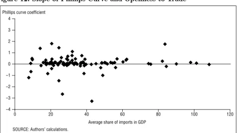
puzzle. Figure 12 presents the basic evidence. Here we plot estimates of the slope of the Phillips curve in various countries against the degree of

openness of the country, as measured by the share of imports in GDP.16

There clearly is no meaningful relationship between the two.

Loungani, Razin, and Yuen (2001) examine the relationship between the sacrifice ratio and another measure of openness—openness to capital flows. They find that countries with more capital controls have lower sac-rifice ratios (steeper Phillips curves) on average. The authors also use the measure created by Ball, Mankiw, and Romer (1988) and base their em-pirical work on a sample of thirty-five countries. As countries become more open to international capital flows, the sacrifice ratio seems to increase, or the Phillips curve becomes flatter, contrary to the mechanism that is central to the Romer story.

15 _{Indeed, Ball (1994) also looks at the relationship between his measure of the}

sacrifice ratio and openness as measured by Romer (1993) and is unable to find a significant relationship.

16 _{Specifically, for each country we plot the estimate of the coefficient γ from the simple}

regression ∆πt=γGapt –1+εt, where Gap is measured as the deviation of GDP from a trend

defined using the Hodrick–Prescott filter along with the country’s ratio of imports to GDP. This is, of course, a simplification. As conventionally measured, the sacrifice ratio depends not only on the slope of the Phillips curve, shown in Figure 12, but also on the persistence of inflation.

Staff

PAPERS

Federal Reserve Bank of Dallas

1

Figure 12: Slope of Phillips Curve and Openness to Trade

0 20 40 60 80 100 120 –4 –3 –2 –1 0 1 2 3 4

SOURCE: Authors’ calculations. Phillips curve coefficient

Average share of imports in GDP

Karras (1999) presents evidence more supportive of the Romer story. He examines the relationship between money growth and output in a sample of thirty-eight countries over the period 1953–90. He finds that the more open economies are (as measured by the share of imports in GDP), the smaller the effect a change in the money stock has on output. This would be consistent with a steeper Phillips curve in more-open economies, but Karras’ results need to be interpreted with caution, given the poten-tial endogeneity of his measure of the money stock, M1.

Subsequent work by Razin and Yuen (2002) presents theoretical rea-sons we should expect to see the sacrifice ratio increase with openness. Their model extends the model Woodford (2003) developed to an economy with international trade and capital mobility. They derive expressions for the domestic Phillips curve under three alternative assumptions about openness: complete capital and goods mobility, closed capital account but open trade account, and closed trade and capital accounts. Under the last assumption, the domestic Phillips curve depends on inflation

expecta-tions and the domestic output gap.17 _{With an open trade account and}

internationally mobile capital, the domestic Phillips curve will depend on the foreign as well as the domestic output gap and the real exchange rate. Important for our perspective, the slope of the Phillips curve declines as the country becomes more open to trade and capital flows. The fraction of goods produced domestically is the key parameter determining how much flatter the Phillips curve is in the economy with complete mobility of goods and capital than in the economy closed to both. The smaller this fraction, the flatter the Phillips curve in a globalized world.

Evidence for the U.S.: Phillips Curve Models

The evidence reviewed above suggests a significant correlation between the degree to which an economy is open to world markets and its long-run inflation rate. However, by all the measures looked at and many others,

17 _{The output gap concept in this model is the same as that Woodford (2003) uses—i.e.,}

Staff

PAPERS

Federal Reserve Bank of Dallas

1

the United States is not a very open economy, which raises the question of

whether global developments really matter all that much for inflation in

the U.S. As the introduction notes, there have been a number of attempts

to isolate globalization’s effects on U.S. inflation. One of the earliest to do so was Tootell (1998), who asks whether globalization could account for the missing inflation of the late 1990s. Using a standard Phillips curve ap-proach, he finds little evidence that globalization—specifically, measures of foreign slack—helps determine U.S. inflation. Tootell’s sample period covers 1973–96, thus missing much of the acceleration in globalization that has occurred in the past decade. Perhaps more important, he only considers slack in the other G-7 countries (Japan, Germany, U.K., France, Italy, and Canada). While these countries accounted for about half of U.S. imports over the period Tootell looks at, by 2005 they accounted for only 37 percent. Using similar methodology but a different sample period, Gamber and Hung (2001) reach the opposite conclusion. They find that globalization helped hold down U.S. inflation in the late 1990s.

Both Tootell and Gamber and Hung use a traditional backward-look-ing Phillips curve model to address the question of whether and how glo-balization matters for U.S. inflation. This Phillips curve is usually speci-fied as (6) π_t α βπ_{i t i} γ_{i t i} ε i k t t i k Slack L Z = + ₋ + ₋ + + = =

∑

∑

where Θ(L)= [θ₁(L), θ₂ (L),…,θ_N(L)], θ_j(L)is a polynomial in the lag

oper-ator L, and Z_t′=[Z_1,t,Z_2,t,…,Z_N,t] are additional explanatory variables, such

as dummy variables for price controls, oil prices, and the terms of trade. The lagged inflation terms are often interpreted as capturing the effect of expected inflation, with expectations assumed to be backward looking.

The constraint

Σ

i=11βi=1 is often imposed to ensure no long-run trade-off

between Slack and inflation. The variable Slack is usually measured as the unemployment or capacity utilization rate, or the deviation of these series from some estimate of their natural or long-run rate, or the deviation of aggregate output from some estimate of potential or trend. There is little consensus on what variables belong in Z. The choice is usually dictated by a desire to improve the fit of some previously estimated version of the traditional model or the desire to evaluate the incremental explanatory power of some new variable.

One way of thinking about how globalization might matter for do-mestic inflation developments would be to argue that the traditional Phil-lips curve model is only useful in explaining the evolution of the prices of domestically produced goods, with the prices of imported goods

be-ing determined on world markets. Thus, overall inflation, π, would be

viewed as a weighted average of the inflation rate of domestically

pro-duced goods and services, πDomestic_{, and import price inflation, π}Import _:

π =(1–ϕ)πDomestic _+ϕπImport_{, where ϕ represents the share of imports. This}

is essentially the approach Tootell and Gamber and Hung take, although they go one step further by distinguishing between oil and non-oil imports.

Staff

PAPERS

Federal Reserve Bank of Dallas

0

Tootell argues that the distinction is important, insofar as oil prices over the period he looks at (1973–96) were determined primarily by geo-political considerations, rather than global capacity utilization. The prices of non-oil imports, on the other hand, might be expected to be more re-sponsive to measures of global slack.

Tootell estimates a version of equation 5, with oil prices and a mea-sure of global slack included as elements of the Z vector. He meamea-sures slack in terms of deviation from a constant, natural rate of unemployment in the other G-7 countries and finds no statistically significant relationship with U.S. inflation. Column 1 of Table 1 reports our attempt to replicate the results in his Table 2; we come close but cannot do so. The sum of the estimated coefficients on the foreign output gap, –0.04, is close to his estimate of –0.05. It is also statistically insignificant. We find that the sum of the coefficients on the domestic unemployment rate is –0.10, with a p value of 5.6 percent; Tootell estimates the sum as –0.11 and finds it is significant at the 5 percent level.

Column 2 of Table 1 reports what happens when we extend the sam-ple to include the past ten years. Note that the sum of the coefficients on the domestic unemployment rate declines to –0.06 and is now significant only at the 10 percent level. This is consistent with the evidence presented above. The sum of the coefficients on the foreign output gaps rises in (absolute) magnitude to –0.07, with a p value of 2.9 percent. That is, add-ing observations from the period with the most dramatic acceleration in globalization causes foreign-output-gap variables to show up as significant in Tootell’s specification.

Table 1: Estimating Global Slack’s Effect on U.S. Inflation: Tootell’s (1998) Model

(1) (2)

Constant .66 (2.3) .35 (2.3)

U.S. unemployment –.10 (5.6) –.06 (5.2)

Lagged inflation 1 1

Oil import price inflation .98 (2.2) .17 (0.2)

Foreign output gap –.04 (1.5) –.07 (6.3)

Nixoff .72 (2.9) .79 (3.8)

Sample period 1973:Q3–1996:Q2 1973:Q3–2006:Q1

Number of observations 92 131

R–2 _{.79 .84}

Log likelihood –17.51 –13.81

NOTES: Dependent variable is the quarter-to-quarter change in the Consumer Price Index excluding food and energy. Coefficients on two lags of the unemployment rate are summed;

t statistics in parentheses, F statistics in the case of summed coefficients. Sum of the

coefficients on 12 lags of the dependent variable constrained to add to 1. Foreign output gap measured as the trade-weighted deviation of unemployment from the estimated NAIRU in Canada, France, Germany, Japan, Italy, and the U.K. Nixoff is a dummy variable capturing the quarter when wage and price controls were lifted.

Staff

PAPERS

Federal Reserve Bank of Dallas

1

We should be careful about reading too much into this, however. To begin with, Tootell’s measure of foreign slack covers only the other mem-bers of G-7. While these countries accounted for about half of U.S. im-ports in the 1970s and ’80s, that share has since declined to just over one-third, with countries like China growing in importance. Second, Tootell measures slack in terms of the deviation of unemployment from a constant NAIRU. An examination of the history of unemployment and inflation in the other G-7 countries suggests that the NAIRU is unlikely to be constant but instead evolves over time as demographics and labor market institutions change.

Gamber and Hung (2001) also estimate traditional backward-looking Phillips curves to assess the importance of global slack for U.S. inflation developments. They estimate a generously parameterized model, with

for-eign slack measured as a trade-weighted average of capacity utilization

in the United States’ thirty-five major trading partners, including such countries as China, India, Brazil, and Russia. They find that their measure of foreign excess capacity has additional explanatory power even after con-trolling for the price of non-oil imports, the prices of food and energy, and the deviation of labor productivity growth from trend. They consider this evidence that foreign excess capacity has tended to lower U.S. inflation through channels other than the traditional import price channel.

We were unable to replicate and update Gamber and Hung’s results. An attempt to construct measures of slack for a wider range of countries than those in the OECD rapidly runs into severe data constraints. Some of the newly emerging economies lack comprehensive sets of national ac-counts or only have data for short spans or report high frequency (e.g., quarterly) data in a way that makes it difficult to separate the trend from

the cycle. For example, China only reports real GDP data in levels at

an annual frequency starting in 1978; quarterly real GDP data are only reported on a twelve-month-change basis starting in 2000. Russia reports quarterly real GDP in levels, but only starting in 1995.

To examine whether U.S. inflation developments are more correlated with some measure of global slack than with some measure of domestic slack, we constructed a world-output-gap variable using data on real GDP at an annual frequency for a group of major U.S. trading partners—the euro area, the U.K., Canada, Japan, Mexico, China, India, and Brazil. Combined, these countries account for more than 80 percent of U.S. im-ports. (China, Mexico, Brazil, and India alone account for more than 30 percent; in 1995, for only 17.7 percent.)

We constructed a world-output-gap variable using annual real GDP data for this group of countries, detrending the data using the Hodrick–

Prescott filter with a smoothing parameter equal to 100, then combining

the individual country gaps thus estimated using trade weights.18

18 _{The measure of the U.S. output gap constructed using the HP filter is very highly}

correlated with the measure of the U.S. output gap constructed using a production function approach and reported by the OECD in its semiannual Outlook. The pairwise correlation between the two series is 0.96.

Staff

PAPERS

Federal Reserve Bank of Dallas

Figure 13: Estimates of U.S. and Global Output Gaps

–2 –1.5 –1 –.5 0 .5 1 1.5 2 2.5 3 2005 2004 2003 2002 2001 2000 1999 1998 1997 1996 1995 1994 1993 1992 1991 U.S. Global Percent

SOURCE: OECD Economic Outlook.

Figure 13 plots the estimated gap series, along with a measure of the U.S. output gap constructed in the same manner. Note that the two series are highly correlated, with a pairwise correlation coefficient of 0.67. Table 2 reports the correlation between various measures of the U.S. price level and inflation and our measures of U.S. and global slack.

There seems to be no systematic relationship between the cyclical component of inflation and the U.S. output gap. The correlations are negative or positive, depending on which measure of the price level is used. Column 2 of Table 2 reports the correlations between the U.S. output gap and the change in inflation. This is the basic correlation at the heart of traditional backward-looking accelerationist Phillips curve models. As we see, the correlations are all positive and of the magnitude commonly found in the literature—that is, U.S. inflation tends to increase when U.S. output is above trend.

The last two columns in the table report the same correlations, but with our measure of the world output gap. We do not see the sizable correlations between the change in inflation and the measure of the world output gap (column 4) that we saw between the change in inflation and the measure of the U.S. output gap. Indeed, in some cases the correlations run counter to what might be expected based on the traditional accelerationist model. However, note that there seems to be a fairly robust positive correla-tion between the cyclical component of inflacorrela-tion and the world output gap. The correlation coefficients range from 0.32 to 0.55, depending on the measure of the price level. (By comparison, the correlation between the change in inflation and the U.S. output gap ranges from 0.34 to 0.66.)

This is consistent with what a number of other researchers have found.For

example, Balakrishnan and Ouliaris (2006) argue that changes in global trade and factor markets have affected the business-cycle component of U.S. inflation more than the trend component. Likewise, Borio and Filar-do (2006) Filar-document an increased correlation between measures of global slack and the cyclical component of inflation for a wide range of countries.

Staff

PAPERS

Federal Reserve Bank of Dallas

Table 2: Correlation Between Output Gaps and Inflation

Correlation of U.S. output gap with Correlation of world output gap with Detrended inflation rate (1) Change in inflation rate (2) Detrended inflation rate (3) Change in inflation rate (4) Consumer Price Index .27 .34 .52 –.34 Consumer Price Index excluding food and energy

–.19 .66 .55 .02 Personal Con-sumption Expen-ditures deflator .07 .54 .43 –.31 Personal Con-sumption Expen-ditures deflator excluding food and energy –.27 .66 .32 .08 GDP deflator –.07 .60 .34 –.20

NOTES: Sample period for U.S. is 1970–2005, for world, 1991–2005. Annual data detrended using HP filter with smoothing parameter equal to 100. Change in inflation rate measured as

π_{t +1}–π_t. Sources for the CPI and CPI excluding food and energy are Haver Analytics series PCURS and PCULFER.

4. CONCLUSIONS AND DIRECTIONS FOR FUTURE RESEARCH

This article provides a preliminary review of the literature on global-ization and inflation. We document the trend toward greater integration in recent years, at both the world and U.S. levels, then review the various channels through which greater economic integration might impact infla-tion in the United States. We start with an evaluainfla-tion of the claim that more-open economies tend to have lower inflation in the long run. There is clearly a negative correlation in the cross-country data between openness and long-run inflation. We also present some tentative evidence that it is not just openness to trade that is correlated with lower inflation but also openness to labor and capital flows.

In the final section of the paper, we ask whether there is evidence that global slack is important in explaining the U.S. inflation picture of recent years. We find some evidence that global slack does matter, especially over the past decade and at business-cycle frequencies.

Our evidence should be interpreted with caution, as it is based on simple correlations and reduced-form models. But it does suggest a num-ber of avenues for further research.

1. Measuring openness: What matters? While the cross-country

evi-dence suggests a robust negative relationship between openness and infla-tion, the literature tends to focus on openness to trade. We present some tentative evidence that openness to factor flows (capital and labor) may also matter, but our measures of these flows are far from perfect and have limited coverage. As noted above, ideally, an economy’s openness should be assessed using price data rather than quantity flows, although as Knetter and Slaughter (1999) point out, the data constraints are severe.

Staff

PAPERS

Federal Reserve Bank of Dallas

2. Evaluating the severity of the time-consistency problem in

gen-eral-equilibrium models. To date, the most coherent argument for how

greater openness might lead to permanent reductions in inflation rates has been based on the time-consistency approach to thinking about monetary

policy.While this theory has proven difficult to test empirically, a number

of authors argue that its predictions for how openness may affect inflation offer a useful test. Simple correlations do seem to bear out the theory’s central prediction, but they do not allow us to distinguish between this and other explanations for the global decline in inflation of recent years. Neiss (1999) and Albanesi, Chari, and Christiano (2003a, b) go beyond the reduced-form models of Kydland and Prescott (1977) and Barro and Gordon (1983) to examine the severity of the time-consistency problem in the context of structural general-equilibrium models. Neiss finds that in a model with monopolistic competition and price rigidities, the monetary authorities will set inflation too high if there is no commitment mecha-nism. Albanesi, Chari, and Christiano find that the severity of the time-consistency problem depends crucially on how the demand for money is modeled. An obvious area for further research is to explore the severity of the time-consistency problem in the context of structural models of open economies.

3. The open-economy Phillips curve. A key part of Romer’s (1993)

story about why inflation is lower in more-open economies is that the Phil-lips curve is steeper in such economies, which means that a central bank in such an economy will have less incentive to generate a surprise inflation. However, it is not at all obvious from the data that Phillips curves are steeper in more-open economies. Indeed, Razin and Yuen (2002) present a theoretical model in which the Phillips curve becomes flatter as the economy becomes more open. It would be interesting to see how the corre-lation between infcorre-lation and the cyclical component of infcorre-lation changes in a standard international business-cycle model as economies become more integrated.

4. Discriminating between different explanations of the decline in

global inflation. Both Romer (1993) and Rogoff (2003) use the

Barro–Gor-don model of monetary policy decisionmaking to explain inflation’s world-wide decline over the past decade. Yet as our simple exposition of that model shows, the decline in inflation rates could be due to a myriad of factors: lower target inflation rates, a greater weight on inflation stabiliza-tion than on output stabilizastabiliza-tion, steeper Phillips curves, or a decline in the wedge between the natural and socially optimal output levels. An im-portant area for research is determining how much of the decline in global inflation can be attributed to better monetary policy and how much is due to other factors, such as globalization and perhaps even luck.

5. Structural models of economic integration. In our discussion of

how greater integration might impact U.S. inflation, we sketch out various direct and indirect channels whereby the availability of cheaper imports from foreign countries might lead to lower inflation in the United States.

Staff

PAPERS

Federal Reserve Bank of Dallas

We also point out some potential offsets to these effects. Purely literary or reduced-form analysis does not allow us to say with confidence how these net out. That can only be done in the context of a fully articulated gen-eral-equilibrium model on international trade and capital flows. While tra-ditional trade theory is replete with such models, many are purely static, and few, if any, have a meaningful role for money or monetary policy.

6. Monetary policy in a frictionless world. An important issue not

ad-dressed here is the extent to which the factors driving integration may also undermine monetary policy’s ability to affect real economic activity. The real effects of monetary policy spring from frictions of one sort or another. In many cases, the policy and technology innovations driving the global economic integration also reduce frictions that may have contributed to monetary policy’s ability to affect real activity. The most obvious example is the innovations in information technology that are making prices more flexible. Rogoff (2003) argues that the increased competition resulting from globalization has made wages and prices more flexible, so that mon-etary policy has smaller and less persistent effects on real activity.

Staff

PAPERS

Federal Reserve Bank of Dallas

REFERENCES

Albanesi, Stefania, V. V. Chari, and Lawrence J. Christiano (2003a), “Expecta-tion Traps and Monetary Policy,” Review of Economic Studies 70 (October): 715–41.

———(2003b), “How Severe Is the Time-Inconsistency Problem in Monetary Policy?” Federal Reserve Bank of Minneapolis Quarterly Review, Summer, 17–33.

Ahmed, Shaghil, Andrew Levin, and Beth Anne Wilson (2004), “Recent U.S. Mac-roeconomic Stability: Good Policies, Good Practices, or Good Luck?” Review

of Economics and Statistics 86 (August): 824–32.

Alfaro, Laura (2005), “Inflation, Openness, and Exchange-Rate Regimes: The Quest for Short-Term Commitment,” Journal of Development Economics 77 (June):229–49.

Andersen, Torben M., and Tryggvi Thor Herbertsson (2003), “Measuring Global-ization,” IZA Discussion Paper no. 817 (Bonn: Forschungsinstitut zur Zukunft der Arbeit, July).

Anderson, James E., and J. Peter Neary (2005), Measuring the Restrictiveness of

International Trade Policy (Cambridge Mass.: MIT Press).

Baier, Scott L., and Jeffrey H. Bergstrand (2001), “The Growth of World Trade: Tariffs, Transport Costs, and Income Similarity,” Journal of International

Economics 53 (February):1–27.

Balakrishnan, Ravi, and Sam Ouliaris (2006), “U.S. Inflation Dynamics: What Drives Them over Different Frequencies?” IMF Working Paper no. 06/159 (Washington D.C.: International Monetary Fund, June).

Ball, Laurence (1994), “Credible Disinflation with Staggered Price-Setting,”

American Economic Review 84 (March): 282–89.

Ball, Laurence M., N. Gregory Mankiw, and David H. Romer (1988), “The New Keynesian Economics and the Output–Inflation Trade-off,” Brookings Papers

on Economic Activity, no. 1, 1–65.

Barro, Robert J., and David B. Gordon (1983), “A Positive Theory of Monetary Policy in a Natural Rate Model,” Journal of Political Economy 91 (August): 589–610.

Borio, Claudio, and Andrew Filardo (2006), “Globalisation and Inflation: New Cross-Country Evidence on the Global Determinants of Domestic Inflation” (Bank for International Settlements paper presented at the CEPR/ESI 10th Annual Conference on Globalization and Monetary Policy, Warsaw, Poland, September 1–2).

Burstein, Ariel, Martin Eichenbaum, and Sergio Rebelo (2005), “Large Devalua-tions and the Real Exchange Rate,” Journal of Political Economy 113 (Au-gust): 742–84.

Campillo, Marta, and Jeffrey A. Miron (1997), “Why Does Inflation Differ Across Countries?” in Reducing Infla