ESSAYS ON STRUCTURAL BREAKS AND STABILITY OF THE MONEY DEMAND FUNCTION
by
WAHEED A. BANAFEA
B.S., King Saud University, Riyadh, 2000 M.A., Ohio University, Athens, 2006
AN ABSTRACT OF A DISSERTATION
submitted in partial fulfillment of the requirements for the degree
DOCTOR OF PHILOSOPHY
Department of Economics College of Arts and Sciences
KANSAS STATE UNIVERSITY Manhattan, Kansas
Abstract
This dissertation consists of three chapters. The first chapter surveys recent studies on the stability of the money demand function in selected developing countries. This chapter presents specific details about modeling and estimating the money demand function. Also, reasons behind the mixed results in the literature on the stability of the money demand function are explored as well as providing a guideline for future research on the stability of the money demand function in developing countries.
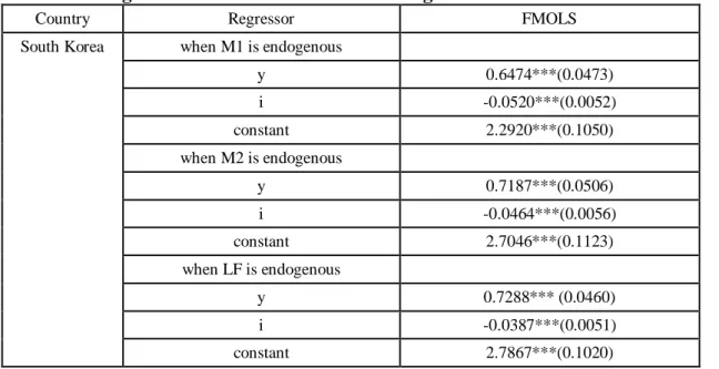
The second chapter empirically investigates the stability of the money demand function in South Korea and Malaysia. The conventional money demand specification and cointegration framework with a single unknown structural break are conducted. The results of the residual-based tests for cointegration reveal that the M1, M2, and M3 demand are stable in the long run in Malaysia. However, there is no evidence of the stability for all three measures of the money demand in South Korea. The results of the residual-based tests suggest that structural breaks in the cointegration vectors are important and need to be accounted for in the specification of the M1, M2, and LF demand in South Korea, where LF includes M2 in addition to the reserves of nonbanking financial institutions and long-term deposits.
The third chapter complements the previous chapter. It aims to evaluate the stability of the money demand function in South Korea and Malaysia using a cash in advance model and cointegration framework with one unknown structural break. This theoretical model adds short-term foreign interest rates and real exchange rates in addition to short-short-term domestic interest rates and real income. Also, the Granger causality and currency substitution analysis are conducted in this chapter. The results of the residuals-based tests indicate that the M2 and LF demand in South Korea, and M1, M2, and M3 demand in Malaysia are stable in the long run.
The structural breaks may not be fairly absorbed when a cash in advance model is used for M1 in South Korea. Thus, the residual-based tests suggest that the structural break is still important and needs to be included in the specification of the M1 demand in South Korea.
ESSAYS ON STRUCTURAL BREAKS AND STABILITY OF THE MONEY DEMAND FUNCTION
by
WAHEED A. BANAFEA
B.S., King Saud University, Riyadh, 2000 M.A., Ohio University, Athens, 2006
A DISSERTATION
submitted in partial fulfillment of the requirements for the degree
DOCTOR OF PHILOSOPHY
Department of Economics College of Arts and Sciences
KANSAS STATE UNIVERSITY Manhattan, Kansas
2012
Approved by: Major Professor Dr. Steven P. Cassou
Copyright
WAHEED A. BANAFEA 2012
Abstract
This dissertation consists of three chapters. The first chapter surveys recent studies on the stability of the money demand function in selected developing countries. This chapter presents specific details about modeling and estimating the money demand function. Also, reasons behind the mixed results in the literature on the stability of the money demand function are explored as well as providing a guideline for future research on the stability of the money demand function in developing countries.
The second chapter empirically investigates the stability of the money demand function in South Korea and Malaysia. The conventional money demand specification and cointegration framework with a single unknown structural break are conducted. The results of the residual-based tests for cointegration reveal that the M1, M2, and M3 demand are stable in the long run in Malaysia. However, there is no evidence of the stability for all three measures of the money demand in South Korea. The results of the residual-based tests suggest that structural breaks in the cointegration vectors are important and need to be accounted for in the specification of the M1, M2, and LF demand in South Korea, where LF includes M2 in addition to the reserves of nonbanking financial institutions and long-term deposits.
The third chapter complements the previous chapter. It aims to evaluate the stability of the money demand function in South Korea and Malaysia using a cash in advance model and cointegration framework with one unknown structural break. This theoretical model adds short-term foreign interest rates and real exchange rates in addition to short-short-term domestic interest rates and real income. Also, the Granger causality and currency substitution analysis are conducted in this chapter. The results of the residuals-based tests indicate that the M2 and LF demand in South Korea, and M1, M2, and M3 demand in Malaysia are stable in the long run.
The structural breaks may not be fairly absorbed when a cash in advance model is used for M1 in South Korea. Thus, the residual-based tests suggest that the structural break is still important and needs to be included in the specification of the M1 demand in South Korea.
viii
Table of Contents
List of Figures ... xi
List of Tables ... xiii
Acknowledgements ...xiv
Dedication ... xv
Chapter 1 - The Money Demand: Theories and Evidence ...1
1.1 Introduction ...1
1.2 Money Demand Function Specification ...3
1.3 Theoretical Models ...4
1.3.1 Quantity Theory ...4
1.3.1.1 Fisher Equation of Exchange ...4
1.3.1.2 The Cambridge Approach ...5
1.3.2 Keynesian Theory ...6
1.3.3 Inventory Theory (The Baumol-Tobin Model) ...7
1.3.4 Friedman’s Theory ...8
1.3.5 Cash in Advance Model ...9
1.4 Current Literature ... 10
1.5 Conclusion ... 23
Chapter 2 - Endogenous Structural Breaks and Stability of the Money Demand Function in a Closed Economy: The Case of South Korea and Malaysia ... 25
2.1 Introduction ... 25
2.2 The Asian Financial Crisis ... 27
2.3 Literature Review ... 29
2.4 The Theoretical Framework ... 34
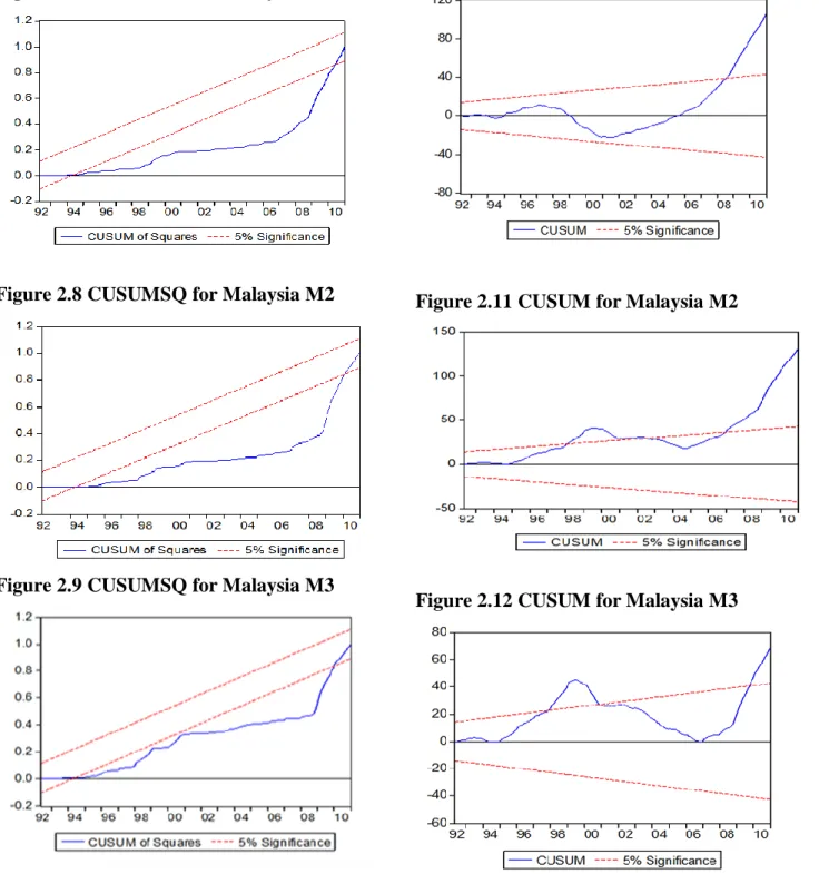
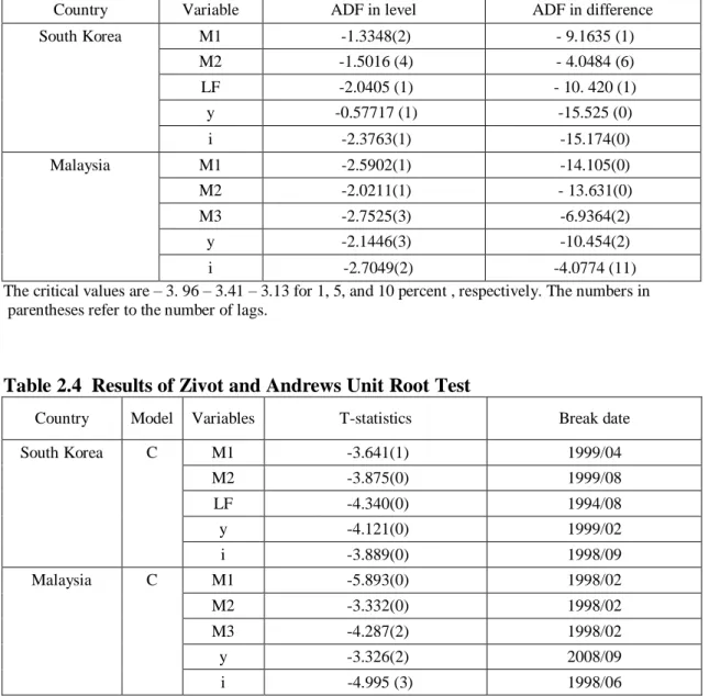
2.5 Unit Root Tests ... 35
2.6 Cointegration Tests... 37
2.6.1 Johansen’s Multivariate Cointegration Test ... 37
ix
2.7 The Model and Data ... 39
2.8 Testing for Structural Breaks ... 40
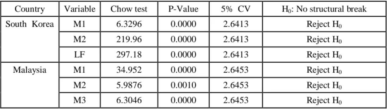
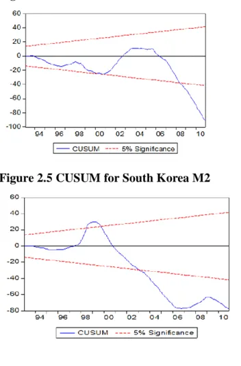
2.8.1 Chow Test ... 40
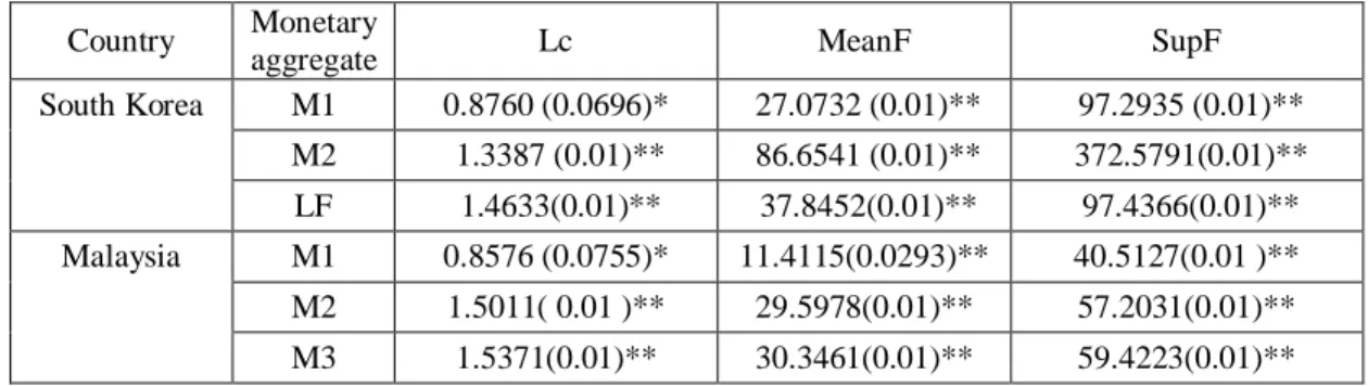
2.8.2 CUSUM and CUSUMSQ Tests for Parameter Instability ... 41
2.8.3 Andrews and Andrews and Ploberger Tests ... 44
2.9 Empirical Results ... 46
2.9.1 Unit Root Tests Results... 46
2.9.2 Johansen and Juselius (1990) Cointegration Test Results ... 48
2.9.3 The Long Run Elasticities before considering Structural Breaks ... 51
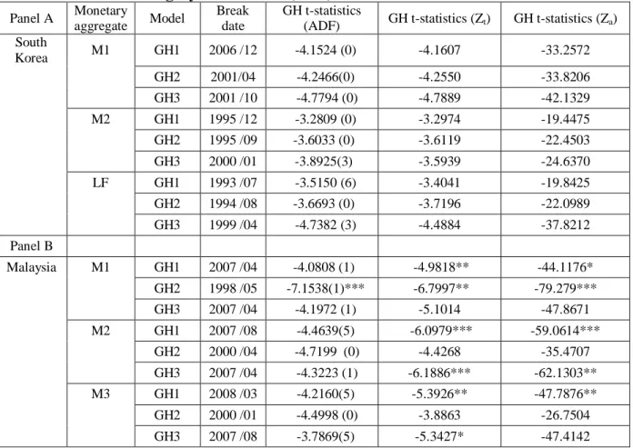
2.9.4 Gregory and Hansen (1996) Cointegration Test Results ... 52
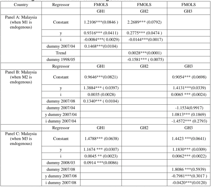
2.9.5 The Long Run Elasticities after considering Structural Breaks ... 56
2.10 Summary and Conclusion ... 58
Chapter 3 - Estimating Money Demand Function in South Korea and Malaysia: Evidence from a Cash in Advance Model with a Cointegration Test allowing for a Structural Break ... 60
3.1 Introduction ... 60
3.2 Theoretical Framework... 63
3.3 Model and Data ... 65
3.4 Econometric Methodologies ... 67
3.4.1 Testing for Structural Breaks and Parameter Instability ... 67
3.4.1.1 Hansen Instability Test ... 67
3.4.1.2 Andrews and Andrews and Ploberger Tests ... 67
3.4.2 Unit Root Tests ... 68
3.4.3 Cointegration Tests ... 69
3.4.3.1 Johansen’s Multivariate Cointegration Test ... 69
3.4.3.2 The Gregory and Hansen Approach... 69
3.5 Long Run and Short Run Granger Causality Tests ... 70
3.6 Empirical Results ... 72
3.6.1 Testing for the Joint Significance ... 72
3.6.2 Parameter Instability Test Results ... 72
3.6.3 Unit Root Test Results ... 75
x
3.6.4.1 The Results of Johansen and Juselius (1990) Cointegration Test ... 78
3.6.4.2 The Long Run Elasticities before considering Structural Breaks ... 81
3.6.4.3 The Results of Gregory and Hansen (1996) Cointegration Test ... 83
3.6.4.4 The Long Run Elasticities after considering the Structural Breaks ... 86
3.6.5 Granger Causality Test Results ... 92
3.7 Summary and Conclusion ... 97
Bibliography ... 100
Appendix A - Supplemental Data for Chapter 1... 108
Appendix B - Supplemental Data for Chapter 2 ... 114
xi
List of Figures
Figure 2.1 CUSUMSQ for South Korea M1 ... 42
Figure 2.2 CUSUMSQ for South Korea M2 ... 42
Figure 2.3 CUSUMSQ for South Korea LF ... 42
Figure 2.4 CUSUM for South Korea M1 ... 42
Figure 2.5 CUSUM for South Korea M2 ... 42
Figure 2.6 CUSUM for South Korea LF ... 42
Figure 2.7 CUSUMSQ for Malaysia M1 ... 43
Figure 2.8 CUSUMSQ for Malaysia M2 ... 43
Figure 2.9 CUSUMSQ for Malaysia M3 ... 43
Figure 2.10 CUSUM for Malaysia M1 ... 43
Figure 2.11 CUSUM for Malaysia M2 ... 43
Figure 2.12 CUSUM for Malaysia M3 ... 43
Figure 3.1 GH1 for the Money Demand M1 in South Korea ... 116
Figure 3.2 GH2 for the Money Demand M1 in South Korea ... 116
Figure 3.3 GH3 for the Money Demand M1 in South Korea ... 116
Figure 3.4 GH1 for the Money Demand M2 in South Korea ... 117
Figure 3.5 GH2 for the Money Demand M2 in South Korea ... 117
Figure 3.6 GH3 for the Money Demand M2 in South Korea ... 117
Figure 3.7 GH1 for the Money Demand LF in South Korea... 118
Figure 3.8 GH2 for the Money Demand LF in South Korea... 118
Figure 3.9 GH3 for the Money Demand LF in South Korea... 118
Figure 3.10 GH1 for the Money Demand M1 in Malaysia ... 119
Figure 3.11 GH2 for the Money Demand M1 in Malaysia ... 119
Figure 3.12 GH3 for the Money Demand M1 in Malaysia ... 119
Figure 3.13 GH1 for the Money Demand M2 in Malaysia ... 120
Figure 3.14 GH2 for the Money Demand M2 in Malaysia ... 120
Figure 3.15 GH3 for the Money Demand M2 in Malaysia ... 120
Figure 3.16 GH1 for the Money Demand M3 in Malaysia ... 121
xii
xiii
List of Tables
Table 2.1 Results of the Chow Test ... 40
Table 2.2 Results of Quandt-Andrews and Andrews-Ploberger Tests ... 45
Table 2.3 Results of Augmented Dickey Fuller Test ... 46
Table 2.4 Results of Zivot and Andrews Unit Root Test ... 46
Table 2.5 Results of Johansen Cointegration Test ... 50
Table 2.6 Long Run Elasticities before considering Structural Breaks ... 52
Table 2.7 Results of Gregory and Hansen (1996) Tests ... 54
Table 2.8 Long Run Elasticities after considering Structural Breaks ... 57
Table 3.1 Results of F-Test ... 72
Table 3.2 Results of Hansen (1992) Test ... 73
Table 3.3 Results of Quandt-Andrews and Andrews-Ploberger Tests ... 74
Table 3.4 Results of Augmented Dickey Fuller Test ... 77
Table 3.5 Results of Zivot and Andrews Unit Root Test ... 77
Table 3.6 Results of Johansen Cointegration Test ... 79
Table 3.7 Long Run Elasticities before considering Structural Breaks ... 82
Table 3.8 Results of the Gregory and Hansen Cointegration Test ... 85
Table 3.9 Long Run Elasticities after considering Structural Breaks ... 90
Table 3.10 Results of Granger Causality Test ... 95
Table A.1 Summary of the Literature Review on the Stability of the Money Demand Function in selected Developing Countries ... 108
Table B.1 Summary of Literature Review on the Stability of the Money Demand Function in South Korea and Malaysia ... 114
xiv
Acknowledgements
I would like to thank my major advisor Dr. Cassou for his guidance and encouragement. Dr. Cassou’s office was always open to me to discuss questions related to my research. I think that I was lucky to work with him. Beside the academic knowledge, I learned from him to always be optimistic and never give up.
I also want to thank my committee members: Dr. William Blankenau, Dr.Lloyd Thomas, Dr.Timothy Dalton, and outside chairperson Dr. Esther Maddux for their valuable comments. My grateful appreciation extends to Dr. Lance Bachmeier for his valuable suggestions.
Special thanks to my mother for her prayers and encouragement. I thank my wife for her support and patience. The smiles of my daughter, Hton, and her brothers, Rakan and Ryan, give me the motivation to work hard and, at the same time, relieve the stress that usually comes with a Ph.D program. For their loving encouragement, I am truly grateful. In addition, I am deeply thankful for my brother, Saleh, for giving me his assistance whenever I needed it.
Finally, I would like to thank my friends Yousef Al-Saadi and Moyd Al-Rsassy for their support and encouragement.
xv
Dedication
I dedicate this work to my mother, wife, and children: Hton, Rakan, and Ryan. Their intangible contribution to my research have made this possible.
1
Chapter 1 - The Money Demand: Theories and Evidence
1.1 Introduction
The relationship between money demand and its determinants is a crucial concern for policymakers, since it allows policymakers to formulate an appropriate monetary policy and increase the level of accuracy in targeting money growth. The issue of the stability of the money demand function in the long run has received extensive attention in the past. However, mixed results are found in the literature. Some studies indicate that money demand is unstable, while others claim it is stable. For instance, Goldfeld (1976) claims that the money demand is unstable in the US during the 1970s; and Stock and Watson (1993) claim that M1 money demand in the US is unstable when post-war data are used. However, when the sample period of Stock and Watson is extended to 1996 by Ball (2001), the results show stability of M1 demand. Ericsson, Hendry, and Prestwich (1998) show that the M2 demand in the UK is stable for the period of 1878 to 1975 despite the two world wars. However, when they evaluate M2 demand on data spanning only 1976 to 1993, they find that M2 demand is unstable. They indicate that the model performs better in the sample period 1878 to 1975 than the 1976 to 1993 period. Thus, they conclude that M2 demand in the UK is unstable over the period 1976 to 1993.
Furthermore, Choi and Jung (2009) find that M1 demand in the US, as it is narrowly defined, is unstable for the period 1959Q1 to 2000Q4. When they estimate the unknown structural break points in the money demand function and test to see if the long run relationship exists in each sub-sample period of the structural break points, they find evidence of stability within each sub-sample but not for the full sample. On the other hand, some studies claim that money demand is stable and that a long run relationship exists between the money balances and
2
their determinants. Orden and Fisher (1993) find evidence of a long run relationship between M3 money demand and its determinants in New Zealand. Moreover, Ericsson and Sharma (1998) find that the M3 money demand is stable in both the long run and the short run in Greece.
Some studies attribute the instability of the money demand function to structural changes arising from innovations in the financial sector and financial deregulation (Boucher and Lippert (1996); Ericsson, Hendry, and Prestwich (1998); Cho and Miles (2007); Pradhan and Subramanian (2002); and Chio and Jung (2009)). In addition, Haug and Lucas (1996) show that the stability of the money demand function depends on the type of cointegration tests used and the combination of money and interest rates. Furthermore, the data frequency can play an important role when testing for stability (Gregory and Hansen (1996)). Cheong (2001) infers that the instability of the money demand function could be caused by misspecification in dynamic models, error correction models, that omit important lags.
The purpose of this study is to provide reference points for the stability of the money demand function in developing countries during the 2000s. Thus, this chapter can be helpful to future research on the relationship between the money demand and its determinants. The motivation for writing this chapter is that most of the survey papers on the stability of the money demand function cover the period before 2000 (Goldfeld and Sichel (1990); Laidler (1993); and Sriram (2001)). Therefore, this chapter reviews more recent studies on the money demand function. This chapter presents specific information about theories of the money demand, specification of the money demand, techniques used, the sample period, the frequency of the data, and the long run income elasticities. This information will provide a concise synopsis of recent studies that can be used with future research on the stability of the money demand function and help policymakers to choose an appropriate monetary policy.
3
The chapter is organized in the following manner. Section 2 discusses the specification of the money demand function, theories of the money demand are presented in Section 3, and Section 4 discusses the current literature. Finally, section 5 provides the conclusion.
1.2 Money Demand Function Specification
The general specification of the money demand function can be written in the following form:
(M/P) = f (scale variable, opportunity cost variables) (1.1) where M is the nominal monetary aggregate, P is the price level. Sriram (2001) indicates that economic theory does not suggest a specific form for the money demand function. However, Zarembka (1968) indicates that there is a general consensus that Equation (1) can take the log-linear form, and other studies suggest a non-log-linear specification to be the most appropriate model (Pradhan and Subramanian (2002); Chen and Wu (2005); and Austin et al. (2007)) since the non-linear models provide a better fit than non-linear models, and non-linear models may not be appropriate in the presence of the structural breaks.
As there is a general consensus on forms for the money demand function, most of the recent studies use either the log-linear or the semi-linear models, and a few studies use non-linear models (Austin et al. (2007) and Miteza (2009)). In empirical studies, both the real money balances and the scale variable are in logarithms, while nominal interest rates variables are in linear form. Accordingly, the coefficient on the scale variable is interpreted as the income elasticity, and the coefficient on the opportunity cost variable is interpreted as semi-elasticity. The choice of the opportunity cost variable is crucial especially when examining the stationarity of the money demand in the short run (Ball (2002)). However, Hoffman et al. (1995) show that the choice of the opportunity cost variable is not critical when evaluating the stationarity of the money demand function in the long run.
4
1.3 Theoretical Models
1.3.1Quantity Theory
The quantity theory is presented by classical economists and hypothesizes that there is a direct and proportional relationship between the quantity of money and the price level. This relationship was developed by two classical economists, Fisher and Pigou.
1.3.1.1Fisher Equation of Exchange
The Fisher equation of exchange can be written as
M V = P T, (1.2) where M is the quantity of money, V is the transactions velocity of money, P is the price level, and T is the number of transactions. Money is neutral and only can be used to facilitate transactions. Thus, Fisher emphasizes only one of the functions of money, the medium of exchange function.
Since it is hard to measure the number of transactions, T, economists use income (output) , y, instead of the number of transactions (Mankiw p. 83). Thus, the quantity equation can be written as
M V = P y. (1.3) V is now the income velocity of money, rather than the transactions velocity. Fisher assumes that the velocity of money is constant in the short run because the velocity is affected by institutions that change slowly over time. Also, he assumes that total output is constant in the short run, as the flexibility of prices and wages causes the output to be at the full employment level. Under these assumptions, Equation (3) shows that a change in the quantity of money, M, leads to an equal percentage change in the price level, P. Fisher believes that interest rates do not affect money demand in the short run.
5 1.3.1.2The Cambridge Approach
The Cambridge approach is attributed to two Cambridge economists, Alfred Marshall and A. C. Pigou. They focused on two of the functions of money. Money serves as a medium of exchange, and individuals use it to facilitate transactions. Accordingly, they agreed with Fisher’s view that the money demand is proportional to nominal income. Also, they emphasize that money functions as a store of wealth. Therefore, they suggest that the demand for money is affected by wealth. When wealth increases, people tend to store it by holding assets, and money is considered to be one of these assets. Marshall and Pigou assume that nominal wealth is proportional to nominal income and that the wealth component of the demand for money is proportional to nominal income. Thus, the money demand is proportional to nominal income. According to their view, the money demand can be written as
M = k P y, (1.4) where k is a constant that represents how much money individuals want to hold for every dollar of income. Equation (4) states that the quantity of nominal money balances is proportional to nominal income. What distinguishes the Cambridge approach from the Fisher equation of exchange is that Cambridge approach allowed k to fluctuate in the short run, meaning that velocity is not constant in the short run. This is due to the second function of money, store of wealth, since decisions about storing wealth in money depend on yields and expected returns on other assets. Thus, the Cambridge economists believe that both interest rates and nominal income affect money demand.
6 1.3.2Keynesian Theory
Keynesians assume that there are three motives for holding money. First, they agreed with Fisher and the Cambridge economists that money is a medium of exchange. Thus, money is held to facilitate transactions; this is called the transaction motive. The expected relationship between income and money demand is positive because an increase in income and expenditures requires people to hold more money. Keynesians’ second motive for holding money is the precautionary motive, which shows that people hold money for unexpected events. The precautionary motive depends on the expected amount of transactions that people want to make in the future. Therefore, the relationship between precautionary money demand and income is positive. The third Keynesian motive is the speculative motive or liquidity preference; this motive emphasizes that money functions as a store of wealth. Keynesians believe that people can store wealth in either money or bonds. Money can be less attractive than bonds, when interest rates are high. However, when interest rates are low, money is considered to be more attractive than bonds. In essence, when interest rates are high, people expect that interest rates would fall in the future so that bond prices would increase. When interest rates are low, people expect that interest rates would increase in the future and bond prices would decrease. Accordingly, there is an inverse relationship between money demand and interest rates. The money demand function under the Keynesian theory can be written as
(M/P) = f (y, i), (1.5) where (M/P) is real money balances, and i is interest rate. What distinguishes Keynesians thought from Fisher’s is that both interest rates and income play an important role in determining money demand. Thus, velocity is not constant in the short run and fluctuates with interest rates. High interest rates reduce speculative money demand and thus increase velocity.
7
1.3.3Inventory Theory (The Baumol-Tobin Model)
Building on Keynes’ theory, William Baumol (1952) and James Tobin (1956) independently recognized that the choice of when and how often to exchange bonds for money is an important choice for individuals. They argued that the benefit of holding money is convenience and that the cost is the interest income foregone by holding money rather than holding interest-yielding assets. They assume that each exchange of interest bearing bonds for money involves a brokerage fee or transaction cost. Thus, larger money balances may decrease the transaction costs, but this would increase the interest income foregone. The individual aims to minimize the brokerage fee and the interest income foregone. This can be expressed by the following well-known square root formula
(M/P) = √ (1.6) where b is the brokerage fee. Equation (6) suggests that the demand for real money balances is proportional to the square root of real income (y) and inversely proportional to the square root of the interest rate (i). There would be no demand for money when the brokerage costs are zero. Therefore, transaction costs play an important role in determining the money demand. The money demand emerges from a tradeoff between interest earnings and transaction costs. In addition, what distinguishes the Baumol-Tobin model from the quantity theory is that the Baumol-Tobin model implies economies of scale in the money demand and a non-zero interest elasticity1. This difference between the Baumol-Tobin model and the classical quantity theory of money led Karl Brunner and Allan Meltzer (1967) to reformulate the Baumol-Tobin model. Brunner and Meltzer show that for large values of real income, y, or small values of transaction
1
According to the Baumol-Tobin model, the economies of scale can be defined as a rise in real spending leads to a less than proportionate increase in real money balances (The coefficient of the real income equals to 0.5).
8
costs, b, there will be no economies of scale in the use of money. In the Brunner-Meltzer view, the Baumol-Tobin model is not considered to be an alternative to the classical quantity theory but implies it. However, Baumol-Tobin would disagree on the basis that changes in interest rates initiated by changes in the money supply, would invalidate the strict quantity theory outcome. 1.3.4Friedman’s Theory
Milton Friedman believed that money demand is a function of wealth and expected returns on other assets relative to the expected return on money. Thus, the specification of the money demand function can be written as
(M/P) = f (yp, ise- im, ibe – im, πe – im), (1.7) where yp is the permanent income; ise is the expected returns on stocks; im is the expected returns on money; ibe is the expected returns on bonds; and πe is the expected inflation rate.
The expected relationship between permanent income and the demand for money is positive. According to this theory, permanent income is considered to be the long run average of both current and expected future income. Therefore, changes in permanent income will not be the source of instability of the money demand. The expected relationship between the money demand and the expected return on bonds, stocks, and goods relative to the return on money is negative. When the return on bonds, stocks, and goods relative to the return on money increases, the quantity of money demanded decreases. Friedman assumed that the expected return on money, im, depends on the interest payments on checkable deposits and services provided by banks on deposits. Unlike Keynesian theory, Friedman believed that changes in interest rates have little or no effect on the money demand. Thus, the money demand is stable and insensitive to changes in interest rates.
9 1.3.5Cash in Advance Model
According to Hueng (1998), a cash in advance model has three advantages. First, it provides a broad specification of the money demand function, since it adds more variables as determinants for money demand.
Second, it explicitly models the liquidity services provided by money through the agent’s budget constraint instead of the utility function. The rationale is that it is the service that provides utility to agents rather than money itself.
Finally, it allows researchers to determine the effect of the interest rate on money demand using comparative statics.
Hueng (1998) believes that the money demand function can be expressed as
(M/P) = f (y, y*, i, i*, q), (1.8) where y denotes the domestic output and y*denotes the foreign output. The variables iand i* refer to the domestic and foreign interest rates, respectively, and q denotes real exchange rates. The relationship between the money demand and income is expected to be positive, indicating that an increase in income increases the demand for money. The expected relationship between the domestic interest rate and money demand is negative because an increase in the domestic interest rate increases the opportunity cost of holding money. On the other hand, the expected relationship between foreign interest rates and the money demand is positive, indicating that an increase in foreign interest rates decreases the opportunity cost of holding money. The effect of the real exchange rate is indeterminate. Thus, the relationship between money demand and the real exchange rate can be positive or negative.
10
1.4 Current Literature
Most of the studies on the stability of the money demand function provide mixed results. This section highlights current studies with a focus on the techniques selected, frequency of the data, measures of the money demand, scale variable, opportunity cost variables, and findings. Focusing on these specific details may lead to a clear answer about the reasons behind these mixed results.
Table A.1 in appendix A summarizes the reviewed literature on the stability of the money demand in selected developing countries. Specifically, Table A.1 provides information about the measures of money, frequency of the data, determinants of the money demand, unit root and cointegration tests, stability tests, long run income elasticity, and the main findings. This information summary may help researchers to have a better idea about how to model and estimate the money demand function in developing countries. For instance, some of the studies use the inflation rate instead of the domestic interest rates as a proxy for opportunity cost, while others use both. Domestic interest rates are controlled by the government and heavily administered in developing countries. Moreover, administrative nominal interest rates in most of developing countries are not adjusted for changes in inflation. Thus, the real interest rates become negative. As a result, they are not reliable (Hossain and Chowdhury (1996); Austin et al. (2007); Baharumshah et al. (2009); and Darrat and Al-Sowaidi (2009)). Based on the determinants of the money demand, we can conclude that most of the studies on the stability of the money demand function do not depend on theoretical models. Consequently, the studies may get mixed results.
Most of the recent studies conduct both cointegration and stability tests to examine the issue of the stability of the money demand. It is worth noting that most of these studies deal with structural breaks exogenously by adding dummy variables to the model; however, a few studies
11
use cointegration tests that take into account these structural breaks (Pradhan and Subramanian (2002); Ramachandran (2004); and Lee and Chien (2008)).
Using data for India, Pradhan and Subramanian (2002) study the stability of the money demand function in India using monthly data covering the 1970:04-2000:03 period. They use two cointegration techniques to investigate the stability of the money demand function in the long run. However, they find mixed results. The Johansen test reveals that both M1 and M3 are cointegrated with their determinants, industrial production, nominal long run interest rates, real exchange rate, foreign interest rates, and the price level. Yet, Gregory and Hansen (1996) show that only M1 is cointegrated with its determinants. They conclude that structural breaks are important and need to be accounted for in the specification of money demand using a non-linear specification.
A study by Ramachandran (2004) establishes a stable demand for M3 in India in the long run during the 1951-2001 period using annual data. Stability and cointegration tests are conducted. To examine the stability of the parameters, the author estimates the real money demand function and the results of the recursive residuals, one-step and N-step forecast tests indicate that the money demand was unstable during the 1978-1980 period. Also, the results of CUSUM test show that the demand for M3 was unstable during the 1991-1995 period, coinciding with the reform period in India. The results of Johansen and Juselius (1990) and Gregory and Hansen (1996) are consistent with what Pradhan and Subramanian (2002) found in their paper, even though they use a different specification of the money demand. Ramachandran (2004) defines the specification of the money demand such that the nominal money demand is a function of real income and the price level. The results of Johansen and Juselius (1990) reveal that there is more than one cointegration vector. However, the results of Gregory and Hansen
12
(1996) show that the null hypothesis of no cointegration can not be rejected. The author mentions that the instability of M3 is transitory since it is caused by the structural breaks that occurred during the 1978-1980 period and found by both the stability and Gregory and Hansen (1996) tests. Thus, the demand for M3 is stable in the long run in India.
Austin et al. (2007) investigate the stability of the money demand function over the 1987-2004 period in China using quarterly data. They use different specifications of the money demand function. First, the linear form of the money demand M0 is tested by Johansen (1991) and the results show that there is at most one cointegration relationship between the real M0 and its determinants, real GDP and inflation rate. Next, the STR model (Smooth Transition Regression) is used as a non-linear model and estimated by conditional maximum likelihood2. The results confirm that the money demand M0 is stable in China. Finally, Austin et al. test the parameter constancy using the auxiliary regression equation. The test results are consistent with the previous findings and reveal stability of the money demand function in China.
Another study by Baharumshah et al. (2009) focuses on the stability of the money demand function in China over the 1990Q4-2007Q2 period using quarterly data. They conduct the autoregressive distributed lag model (ARDL) cointegration procedure proposed by Pesaran et al. (2001) in addition to Hansen (1992) and CUSUM and CUSUMSQ stability tests. Baharumshah et al. stress the importance of the specification of the money demand function. The authors identify the money demand function as a linear model examining the long run relationship between the real M2 demand and its determinants, real GDP, short-term domestic and foreign interest rates, and stock prices. They believe that the inclusion of the stock prices in the model would improve the specification of the money demand function in China. This
2
13
research deals with foreign interest rates as a substitution for theexchange rate. Thus, the impact of the foreign interest rate is expected to be negative3. Moreover, the inflation rate, instead of the domestic interest rate, is used as a measure of the opportunity cost of holding money. Before including stock prices in the model, the results of Pesaran et al. (2001) cointegration tests show that the variables in the M2 model are cointegrated, while the results of the CUSUM and CUSUMSQ tests show that the parameters of the M2 money demand function are unstable. However, after including stock prices in the model, the results of the cointegration and stability tests become consistent and indicate that M2 demand is stable in China.
Lee and Chien (2008) also evaluate the stability of M1 and M2 demand in China using annual data covering the 1977-2002 period. Two different cointegration techniques are used, Johansen (1988) and Gregory and Hansen (1996). The results from the Johansen test suggest that there is one cointegrating vector, implying that a long run relationship exists between M1 and M2 demand and their determinants, real GNP and nominal short run interest rate. However, the results of the Gregory and Hansen test indicate that only M2 demand is stable, while M1 demand is not. They mention that the results of the Gregory and Hansen (1996) test suggest that a structural break is important in the cointegration vector and needs to be included in the specification of the money demand function. Accordingly, the authors indicate that the specification of the money demand, which envelopes unstable economic and financial crises and reforms, raises important questions about the relationship between the money demand and its determinants in the long run. The authors attribute the inconsistent results of their paper and
3
The cash in advance model expects the sign on the foreign interest rates to be positive which indicates that an increase in the foreign interest rate decreases the opportunity cost of holding money.
14
previous studies to the specifications of the money demand function, the length of the data, and the econometric techniques used.
Zuo and Park (2011) analyze the stability of the real M2 demand for the sample period 1996Q1 to 2009Q1 using quarterly data in China. They estimate four versions of the money demand models. First, the real M2 demand is assumed to be determined by real GDP, the interest rate, and stock prices, the Benchmark model. Second, the real M2 demand is determined by real industrial value added (IVA), the interest rate, and stock prices. The third model assumes that the real M2 demand is determined by the real GDP (IVA), expected inflation, and stock prices. In the final model, the real M2 demand is determined by real GDP (IVA) and the expected inflation (interest) rate. Zuo and Park find a long run relationship between M2 demand and its determinants for all four models when the smooth time-varying cointegrating approach is used. To take into account the gradual structural breaks, they allow the parameters to evolve smoothly during the time horizon. They find that the income elasticities are around 0.6 - 0.75 which are inconsistent with the result of Baharumshah et al. (2009) (Table A.1).
Using Indonesian quarterly data for M2 demand over the period 1983Q1 through 2000Q4, James (2005) finds evidence of a long run relationship between real M2 demand and its determinants, real GDP, nominal short run domestic and foreign interest rates, and a time trend4. Also, two impulse dummy variables are added to the model to capture the structural breaks that may have occurred in 1990Q4 and 1998Q2. The Pesaran et al. (2001) cointegration test and CUSUM and CUSUMSQ tests are conducted. The author emphasized that the stability of the money demand function could not be found without taking into account the financial liberalization in the specification of the money demand. Narayan (2007) utilizes both the
4
15
Johansen (1988) cointegration test and Hansen (1992) parameter instability test to investigate the stability of the money demand function in Indonesia. Narayan uses annual data that covers the 1970 to 2005 period. The results from the Johansen cointegration test show that there is evidence of a long run relationship between real M1, M2 demand, and their determinants, which are real GDP, nominal short term domestic and foreign interest rates, and real exchange rates. However, the results from the Hansen test show that both real M1 and M2 demand are unstable. The author concludes that both M1 and M2 demand are unstable in Indonesia.
Sriram (2002) analyzes both the long run and the short run demand for M2 in Malaysia. Monthly data that cover the 1973:08 to 1995:12 period are used to examine the long run relationship between real M2 demand and its determinants, including the industrial production index, own-rate (returns on money), the discount rate (returns on other assets), and the inflation rate. The Johansen (1988) and Johansen and Juselius (1990) cointegration tests are conducted. The structural breaks are treated exogenously by adding two dummy variables to the model. The first dummy refers to the structural break that may have occurred in 1994:01 when the Malaysian government introduced a temporary set of control measures to reduce excess liquidity from the banking system. The second dummy denotes the interest rate regime5. The results of trace and maximum eigenvalue tests indicate that there is at least one cointegration vector. In addition, the short run relationship is tested by using an error correction model (ECM). The model is estimated using ordinary least square method, and the results show that M2 demand is stable in the short run. For robustness, the author evaluates the parameter constancy. Therefore, three stability tests are performed to evaluate the stability of the M2 money demand in the long run
5
According to Sriram (2002), the second dummy has a value of zero for 1973:08-1978:09 and 1985:10-1987:01 to indicate the periods of the presence of market controls and a value of one for 1978:10-1985:09 and 1987:02-1995:12 to denote the liberal regime.
16
and the short run. The results indicate that the money demand function is unstable in both the long run and the short run due to the structural changes.
Nair et al. (2008) utilize an autoregressive distributed lag model (ARDL) to test the stability of the money demand function in Malaysia. They use annual data for the period 1970 to 2004 for real M1, M2, M3 demand, and their determinants, which include real GDP and interest rates. The results show that all three measures of money have a long run relationship with their determinants. However, the income elasticities are inconsistent with quantity theory of money for all three measures, since they are not approximately one (Table A.1). Furthermore, Nair et al. find that the interest rates are positively related with M2 and M3 demand, which is inconsistent with theoretical expectations. Moreover, this research also uses the Gregory and Hansen test to investigate whether the stability of the money demand is affected by the Asian financial crisis. However, instead of determining the structural break endogenously, the authors pre-selected the structural break of 1997, which is the date of the Asian financial crisis. The results of the Gregory and Hansen test indicate that there is no long run relationship between the demand for M1, M2, and M3, and their determinants.
In 2009, Manap also studies the stability of the money demand function in Malaysia. He uses quarterly data from 1977Q1 to 2009Q4. The Johansen (1988) and Johansen and Juselius (1992) tests are conducted. The results are consistent with Nair et al. (2008) and posit that there is at least one cointegration vector in the M1 and M2 series. Thus, there is a long run relationship between M1 and M2 demand and their determinants, which include real GDP and short term interest rates. Manap believes that the evidence of cointegration does not necessarily suggest a stable money demand function over time. Therefore, the Hansen parameter instability test is applied. The findings show that M1 demand is stable, while M2 demand is not. The author
17
attributes the instability of M2 to the existence of a structural break caused by the Asian financial crisis.
Hwang (2002) uses quarterly data from 1973Q1 to 1997Q2 to evaluate the stability of the money demand function in South Korea using Johansen (1988) and Johansen and Juselius (1990) cointegration techniques. M1 and M2 are used as proxies for the money demand, while the real GDP is used as a scale variable. For the opportunity cost, the author tries two types of interest rates, short term and long term interest rates. The results show that both real demand for M1 and M2 are unstable when the short term interest rates are used as the opportunity cost. However, when the long term interest rates are used, the results reveal that both real demand for M1 and M2 are cointegrated with their determinants. For the M1 demand model, the income elasticity of -19.35 is implausible, because it is negative and greater than unity in absolute value. The normalized equation with M2 demand as the dependent variable shows the expected signs and significant coefficients. In addition, the error correction model is used to examine the short run relationship between M1 and M2 demand and their determinants, real GDP and long term interest rates. The results indicate that the M1 model is unstable in the short run. However, the results of the CUSUM test indicate that M1 and M2 demand are stable.
Cheong (2003) evaluates the money demand function in South Korea using quarterly data for the period from 1972Q3 to 1997Q7. Using the Johansen (1988) test, Cheong tests the long run relationship between real M2 demand and the determinants of real GDP, a 1-year time deposit rate, a 3-year corporate bond rate, and the inflation rate. The results show that there is only one cointegrating vector in the system. The income elasticity of 1.28 is greater than unity, meaning that the M2 demand in South Korea responds more than proportionally to real income
18
and that there are no economies of scale6. Furthermore, the relationship between M2 demand and its determinants is investigated using an error correction model (ECM) equivalent to a fifth-order autoregressive distributed lag (ADL) model. In the ECM, seasonal dummies are included with real income and interest rates. This model is recursively estimated by one-step residuals with two standard error bands and Chow tests to evaluate the parameter constancy, and the results indicate that the M2 demand is stable. For robustness, two dummy variables are added to the ECM. The first dummy variable is created to capture the period of the financial deregulation in 1981, and the second dummy is created to capture the effect of the massive reduction in regulated banks’ interest rates in 1982. The Chow test is applied, and the results reveal that both dummies are statistically insignificant at the 5% level. Accordingly, these structural breaks do not affect the stability of the money demand, M2, in South Korea.
In 2007, Cho and Miles examine the impact of the financial innovation on the stability of the money demand function in South Korea. This study uses quarterly data that covers the sample period from 1976Q4 to 1998Q3. A Johansen (1988) cointegration test is conducted. To account for financial innovation, the authors add a linear trend to the conventional money demand specification. The results suggest that there is a long run relationship between the real demand for M2 and the determinants that include real GDP, nominal long term interest rate, and the time trend. Thus, the results imply that monetary targeting could be an option in monetary policy choices.
6
Baharumshah et al. (2009) indicate that if the income elasticity equals 1, the finding is consistent with the quantity theory of money. If the income elasticity equals 0.5, the finding is consistent with the Baumol-Tobin inventory theory. Finally, if the income elasticity is greater than 1, money can be considered a luxury good or as a sign of neglecting the effect of wealth in the model specification.
19
Two recent studies examined the M2 demand function in Nigeria. Anorou (2002) investigates the stability of M2 demand and its determinants, industrial production and short term real interest rates. This study covers the sample period in Nigeria from 1986Q2 to 2000Q1. Anorou finds evidence of a long run relationship between real M2 demand and its determinants using the Johansen and Juselius (1990) cointegration test. To investigate parameter constancy, three tests are conducted, including Hansen (1992), Hansen (1991), and CUSUM and CUSUMSQ. The results of all three tests indicate that M2 demand is stable. Chukwu et al. (2010) reevaluate the stability of M2 demand in Nigeria using quarterly data covering the period from 1986Q1 to 2006Q4. They conduct Gregory and Hansen (1996) tests to evaluate the long run relationship between real M2 demand and its determinants, including real economic activity, interest rates swap spread, and inflation rate. The results reveal that M2 demand is stable in the long run. Also, the stability of M2 demand in the short run is examined using the ECM, and the results show that M2 demand is stable in the short run. The results are consistent with Anorou (2002).
Shu Wu et al. (2005) examine the stability of the money demand function in Taiwan. The paper covers the period from 1978Q1 to 1999Q4. The authors focus on the specification of the money demand. Different models are used to test the stability of the money demand function. First, a Goldfeld-type of money demand function is estimated using the Beach and Mackinnons (1978) maximum likelihood estimation method7. The results of the rolling estimation show that
7
Mt = α0 + α1 Mt-1 + β0 y+ β1 i + єt. where Mt denotes the current money demand, and Mt-1 denotes the first lag of the dependent variable. This model is known as the Goldfeld (1973) short run money demand function. According to this model, the money demand is a function of the first lag of the money (the dependent variable), income and interest rates.
20
M1B demand is unstable8. Next, the authors add another explanatory variable to the model, real stock market transactions, yet the results remain unchanged. However, the ARMAX model, a statistics-oriented approach, and the Johansen maximum likelihood estimation method are conducted. The results from both approaches reveal that M1B demand is stable in Taiwan. The authors note that including a constant term in a model with a lagged dependent regressor can produce results that indicate an unstable money demand function.
Using annual data of five developing countries, Bangladesh, India, Pakistan, Srilanka, and Nepal, for M2 demand over the 1974-2002 period, Narayan et al. (2008) finds evidence of cointegration between M2 demand and its determinants, which include real GDP, nominal short term domestic and foreign interest rates, and real exchange rates. The authors treat the structural breaks endogenously by applying Westerlund (2006) panel cointegration tests. The results of a Hansen (1992) test reveal that the money demand function is stable for all the countries except Nepal. Darrat and Al-Sowaidi (2009) utilize the Johansen and Juselius (1990) cointegration test and Hansen and Johansen (1993) parameter constancy test to evaluate the stability of the money demand in Bahrain, the United Arab Emirates (UAE), and Qatar. The study uses annual data covering the period from 1973 to 2005. To control for structural breaks that might be caused by financial developments, dummy variables are added to the money demand specification. In all three countries, the results of the Johansen and Juselius test indicate that there is a long run relationship between real M1 and M2 demand and the determinants that are real GDP, foreign interest rates, and expected inflation rate. The results of the Hansen and Johansen test reveal that both real M1 and M2 demand are stable in Bahrain; this is consistent with the results of the
8
21
cointegration test. However, the results also show that only real demand for M2 in the UAE and real demand for M1 in Qatar are stable.
Hossain (2010) uses Bangladesh annual data for the broad money balances over the 1973-2008 period to evaluate the stability of the money demand function. The author applies two different tests, Johansen and Juselius (1990) cointegration test and Hansen and Johansen (1993) constancy test. The results of the cointegration test show that the long run relationship exists between real broad money balances and its determinants, real GDP, nominal foreign and domestic interest rates, and nominal effective exchange rate9. However, the constancy test shows mixed results; the results of the Hansen and Johansen test reveal that the broad money demand function is unstable, especially during the early 1990s. The author attributes this instability to financial deregulation and financial innovations. However, the results of Hansen and Johansen test turned out to be the opposite and indicate that the money demand function is stable during the early 2000s.
Kumar (2011) examines the stability of the money demand in 20 developing countries; those include South Africa, Cameroon, Jamaica, Rwanda, Kenya, Ethiopia, Egypt, Nigeria, India, Indonesia, Thailand, China, Philippines, South Korea, Taiwan, Bangladesh, Sri Lanka, Nepal, Malaysia and Singapore. Kumar treats the structural breaks exogenously, choosing 1989 and 1995 as the break dates, since the financial reforms were introduced by most of the developing countries in the late 80s and some during the 90s. According to these break dates, the sample is divided into four sub-samples: 1975-1988, 1989-2005, 1975-1994, and 1995-2005. The error correction method is applied to each sub-sample. The results reveal that M1 demand is stable in all 20 developing countries. Both the income elasticity and the interest rate
9
22
elasticity are plausible for all countries, since the income elasticity is around unity and the interest rate semi-elasticity has the expected sign and is statistically significant.
In the most recent studies on the stability of the money demand function in Africa, Dagher and Kovanen (2011) examine the stability of the money demand function in Ghana in both the long run and the short run. The Pesaran et al. (2001) cointegration test and CUSUM and CUSUMSQ parameter stability tests are used. The results of the cointegration and the parameter instability tests are consistent with each other and indicate that M2 demand is stable in both the long run and the short run.
From the above discussion, we can conclude that there are several reasons that contribute to the mixed results on the stability of the money demand function. First, the interpretation of the results can be confusing and conflicting. For example, both Sriram (2002) and Manap (2009) analyze the stability of the money demand function in Malaysia. The results of the cointegration tests suggest that there is a long run relationship between M2 demand and its determinants. However, the results of the parameter stability tests indicate that M2 demand is unstable. Manap (2009) points out that the cointegration between M2 demand and its determinants does not necessarily imply that M2 demand is stable. Hence, Manap (2009) concludes that M2 demand is unstable, while Sriram (2002) indicates that M2 demand is stable in the long run. Also, Narayan (2007) conducts both cointegration and stability tests. The results of the cointegration test suggest that there is a long run relationship between M2 demand and its determinants, while the results of the parameter constancy test indicate that M2 demand is unstable. Hence, he concludes that M2 demand is unstable in Indonesia.
23
Another reason for the mixed results is the specification of the money demand function. For instance, James (2005) and Narayan (2007) examine the stability of the money demand function in Indonesia using different parameter stability tests. James utilizes CUSUM and CUSUMSQ, while Narayan uses Hansen (1992) test. The results of CUSUM and CUSUMSQ suggest that M2 demand is stable, while the results of Hansen test indicate that M2 demand is unstable. These inconsistent results might be due to the specification of the money demand function, since both papers use different specifications of the demand for M2.
Finally, the choice of the opportunity cost and structural breaks are important. Hoffman et al. (1995) indicate that the choice of an interest rate is not critical when evaluating the money demand in the long run. However, Hwang (2002) could not find stability of M1 and M2 demand when the short term interest rate is used as a proxy for the opportunity cost in South Korea. Structural breaks also influence results. Some studies put more weight on the results from the parameter stability tests while these tests do not account for structural breaks10.
1.5 Conclusion
This chapter provides a useful reference for future research on the stability of the money demand function in developing countries. In addition, it includes a discussion of reasonable explanations for the mixed results of the stability of the money demand function. Most of the research reviews on the money demand function cover periods before 2000s, yet this review focuses on the most recent studies on the money demand function. In fact, this chapter goes on to present various theories of the money demand. This information might help future researchers to choose the appropriate theory when formulating their empirical models of the money demand.
10
Breuer and Lippert (1996) point out that most of the parameter stability tests centered on whether the coefficient estimates are stable over time without taken into account the structural breaks.
24
The specific information about the frequency of the data, methodology used, stability tests, unit root tests, cointegration approaches, income elasticity, and the main findings of the various studies is included here and will be helpful to researchers for a quick comparison of the literature. For instance, the researchers will be able to compare their work and methods using this specific information. Thus, this chapter can be considered as a guide to future research on the stability of the money demand function in developing countries.
25
Chapter 2 - Endogenous Structural Breaks and Stability of the
Money Demand Function in a Closed Economy: The Case of
South Korea and Malaysia
2.1 Introduction
In the past decades, interest in whether the money demand function is stable has received extensive attention. Different econometric techniques have been applied to investigate the behavior of the money demand in both the long run and short run. There are many studies on the stability of the money demand function in the literature, and most of these studies show mixed results. Wolff (1987) attributes money demand instabilities to financial innovations. Lippert and Breuer (1996) conclude that instability of the money demand function is due to structural breaks. They indicate that studies that do not account for the structural breaks can lead to biased results and deduce that the money demand function is unstable. It is important to have a stable money demand function, because it has vital implications on monetary policy. In fact, a stable money demand is useful for explaining and forecasting the behavior of interest rates, exchange rates and GDP. Poole (1970) shows that instability of the money demand can prevent policymakers from implementing the appropriate policy and lower the level of accuracy of targeting money growth. If a stable money demand increases the ability of policymakers to prevent money market disequilibrium, then it is worth investigating the stability of the money demand function using different techniques such as a cointegration framework that accounts for structural breaks.
The purpose of this research is to examine the stability of the money demand function using the narrow definition of the money supply, M1, and the two broad definitions of the money supply M2 and M3 (LF). This study examines demand for M1, M2, and M3 (LF) in two of the Asian tiger countries, South Korea and Malaysia, and uses both Johansen and Juselius (1990)
26
and Gregory and Hansen (1996) cointegration tests. The Gregory and Hansen cointegration test incorporates structural breaks. Therefore, this test allows one to empirically investigate the stationarity of the money demand functions after allowing for a one time structural break in the relationship among the three dependent money demand variables, nominal short-term interest rates, and real income.
The motivation for examining the stability of the money demand functions in South Korea and Malaysia is that most studies in the literature that examine the stability of money demand focus on developed countries, and little attention has been paid to developing countries11. Also, South Korea and Malaysia are two of the Asian countries that experienced a severe economic crisis known as the Asian financial crisis that occurred in July 1997. This crisis likely created a structural break, and the Gregory and Hansen (1996) residual-based test can take this into account when testing for stability of the money demand function. Perron (1989) indicates that the presence of structural breaks in a series can lead to misleading results and negatively affect the properties of the stationary series.
There is no clear answer whether South Korea is considered to be a developed or developing country; in fact, there are mixed classifications of South Korea. According to the World Trade Organization (WTO), South Korea is considered to be one of the developing countries. However, there is no specific definition of the term developed or developing countries in the World Trade Organization. The countries which are members of the WTO declare for themselves if they are developed or developing countries (www.wto.org). Recently, South Korea is treated as a developing country in the literature (Kumar (2011)). In contrast, the International Monetary Fund classifies South Korea as one of the developed countries. This classification is
11
27
based on the GDP as valued by purchasing power parity (PPP), the population, and the total exports of goods and services.
This chapter is organized in ten sections. Section 2 briefly discusses the Asian financial crisis; section 3 reviews relevant literature. The theoretical framework of the money demand function is discussed in section 4. Section 5 includes a discussion of the unit root tests, and section 6 explains the cointegration methodologies of both Johansen and Juselius and Gregory and Hansen tests. The model and data are presented in section 7. Section 8 briefly reviews Chow, CUSUM and CUSUMSQ, Andrews (1993), and Andrews and Ploberger (1994) tests. Sections 9 and 10 present the empirical results and the conclusions, respectively.
2.2 The Asian Financial Crisis
South Korea was hit harder by the Asian financial crisis than Malaysia. During 1994-1996, the Korean government allowed Korean banks and firms to borrow from foreign investors to invest in Korean assets. The cumulative foreign supply of capital was at its highest level, $108 billion. Most of the foreign debt was invested in long run foreign assets instead of short run Korean assets. GDP growth fell from eight percent in the period 1994-1996 to six percent over the first three quarters of 1997 and plummeted to 3.9 percent in the last quarter of 1997. In the first quarter of 1998, GDP growth fell to negative four percent and continued falling until the third quarter. Most of this drop occurred in the manufacturing sector, which is weighted heavier than all sectors in GDP. In 1997, a large number of leveraged conglomerates went into bankruptcy and caused severe damage to South Korean financial institutions. Chandrasekhar and Ghosh (1999) indicate that the Korean government dealt with the crisis by adopting a tight monetary policy, so the call rate was increased from 12.5 percent on the first of December to 30 percent on December 24, 1997. The purpose of this policy was to attract foreign investors back
28
to the economy. Also the Korean government adopted a fiscal contraction policy to deal with this crisis. When these two contraction policies failed to correct the economy, the South Korean government adopted a combination of both stimulative fiscal and monetary policy, but these adjustments were too late to prevent the collapse of the GDP. In 1997, corporate bankruptcies were the main reason behind the sharp increase in the non-performing credit of the South Korean banking system
Ping and Yean (2007) indicate that Malaysia was not as badly affected by the Asian financial crisis as South Korea, even though the crisis started with the Malaysian currency. The value of the Malaysian ringgit started to fluctuate rapidly; in June 1997, the value of the ringgit was 2.52 USD and then dropped to 3.20 USD in September 1997. The depreciation of the ringgit continued and reached a new low level of 4.5 USD in January 1998. The Malaysian stock market was negatively affected by the depreciation of the ringgit against the US dollar. Malaysian enterprises were affected by the decline in both the stock market and the currency. These enterprises were unable to pay the interest on loans, so this put a lot of pressure on bank liquidity. As a result, there was a sharp decline in the economy; it went from a 7.3% growth rate in 1997 to -7.4% in 1998. Unlike South Korea, Malaysia formed a National Economic Action Council (NEAC) to deal with this crisis and did not rely on the IMF. The NEAC made some good decisions that led to the recovery of the Malaysian economy. The growth rate of the economy changed from -7.4% in 1998 to 6.1% in 1999, and this increased growth continued afterward.
29
2.3 Literature Review
In the literature, there are several empirical studies on the stability of the money demand function. These studies use different econometric techniques to empirically investigate the stability of the long and short run relationship between the money demand and its determinants. This section provides a brief review some of the recent studies on the stability of the money demand function in South Korea and Malaysia. The studies selected are divided into two groups. The first group includes studies on the stability of the money demand function in South Korea (Hwang (2002); Bahmani-Oskooee (2002); Cheong (2003); Cho and Miles (2007); Miteza (2009); Kumar (2011)). The other group focuses on the stability of the money demand function in Malaysia (Sriram (2002); Tang (2007); Nair et al. (2008); Tang (2009); Manap (2009); Kumar (2011)). Table B.1 in appendix B summarizes these recent empirical studies.
Hwang (2002) conducts the Johansen (1988) and Johansen and Juselius (1990) cointegration tests and CUSUM parameter constancy test to examine the stability of the M1 and M2 demand functions in South Korea using quarterly data from the period 1973Q1 to 1997Q2. Two different measures of the opportunity cost are applied, long term and short term interest rates. When the short term interest rate was used as a proxy for the opportunity cost, the results show that there is no cointegrating relationship between the M1 and M2 demand and their determinants, real income and short term interest rates. However, when the long term interest rate was used as a proxy for the opportunity cost, the results indicate the existence of a long run relationship between M1 and M2 demand and their determinants, real income and long term interest rates. The results of the error correction model (ECM) show that only M2 demand is stable in both the long run and the short run. On the other hand, the CUSUM test shows that M1 and M2 demand are stable. The author suggests that using the long term interest rates as a