An image segmentation and registration approach to cardiac function analysis using MRI

(1)

University of London

Imperial College of Science, Technology and Medicine

Department of Computing

An image segmentation and registration

approach to cardiac function analysis using

MRI

Wenzhe Shi

Submitted in part fulfilment of the requirements for the transfer of Doctor of Philosophy in Computing of the University of London and

(2)

(3)

Abstract

Cardiovascular diseases (CVDs) are one of the major causes of death in the world. In recent years, significant progress has been made in the care and treatment of patients with such diseases. A crucial factor for this progress has been the development of magnetic resonance (MR) imaging which makes it possible to diagnose and assess the cardiovascular function of the patient. The ability to obtain high-resolution, cine volume images easily and safely has made it the preferred method for diagnosis of CVDs. MRI is also unique in its ability to introduce noninvasive markers directly into the tissue being imaged(MR tagging) during the image acquisition process. With the development of advanced MR imaging acquisition technologies, 3DMRimaging is more and more clinically feasible. This recent development has allowed new potentially 3D image analysis technologies to be deployed. However, quantitative analysis of cardiovascular system from the images remains a challenging topic.

The work presented in this thesis describes the development of segmentation and motion analysis techniques for the study of the cardiac anatomy and function in cardiac magnetic resonance (CMR)images. The first main contribution of the thesis is the development of a fully automatic cardiac segmentation technique that integrates and combines a series of state-of-the-art techniques. The proposed segmentation technique is capable of generating an accurate 3D segmentation from multiple image sequences. The proposed segmentation technique is robust even in the presence of pathological changes, large anatomical shape variations and locally varying contrast in the images.

Another main contribution of this thesis is the development of motion tracking techniques that can integrate motion information from different sources. For example, the radial motion of the myocardium can be tracked easily in untaggedMR imaging since the epi- and endocardial surfaces are clearly visible. On the other hand, tagged MR imaging allows easy tracking of both longitudinal and circumferential motion. We propose a novel technique based on non-rigid image registration for the myocardial motion estimation using both untagged and 3D taggedMR images. The novel aspect of our technique is its simultaneous use of complementary information from both untagged and 3D tagged MR imaging. The similarity measure is spatially weighted to maximise the utility of information from both images.

The thesis also proposes a sparse representation for free-form deformations (FFDs) using

(4)

the principles of compressed sensing. The sparse free-form deformation (SFFD) model can capture fine local details such as motion discontinuities without sacrificing robustness. We demonstrate the capabilities of the proposed framework to accurately estimate smooth as well as discontinuous deformations in 2D and 3DCMRimage sequences. Compared to the standard FFD approach, a significant increase in registration accuracy can be observed in datasets with discontinuous motion patterns.

Both the segmentation and motion tracking techniques presented in this thesis have been applied to clinical studies. We focus on two important clinical applications that can be addressed by the techniques proposed in this thesis. The first clinical application aims at measuring longitudinal changes in cardiac morphology and function during the cardiac remodelling process. The second clinical application aims at selecting patients that positively respond tocardiac resynchronization therapy (CRT).

The final chapter of this thesis summarises the main conclusions that can be drawn from the work presented here and also discusses possible avenues for future research.

(5)

Acknowledgements

I would like to thank my supervisor, Prof. Daniel Rueckert, for his sage advice, patient encouragement and insightful guide throughout the course of my research.

I would also like to thank my second supervisor Dr. Philip ”Eddie” Edwards, for his valuable input and important suggestions for these projects.

Sincere thanks also go to Dr. Declan O’Regan of the Robert Steiner MR imaging unit at Hammersmith Hospital, Dr. Simon Duckett and Prof. Reza Razavi at St Thomas Hospital for acquiring the manyMRdata sets used in this report. In addition, thanks to all dear cooperators from Kings College London and University of Oxford.

I would also like to thank my colleagues and friends in the biomedical image analysis group for their help and support. Especially to Dr. Paul Aljabar, Dr. Wenjia Bai, Dr. Kanwal Bhatia, Dr. Luis Pizarro, Dr. Robin Wolz, Kai Pin (Tom) Tung and Haiyan Wang.

(6)

(7)

Dedication

This thesis is dedicated to my family to their emotional and financial support, especially to my father and mother for instilling the importance of hard work and higher education; to my wife for supporting me each step of the way; to my grandma, grandpa who I wish can notice this from the other side of the world.

(8)

‘Rich in Knowledge and Tenacious of Purpose; Inquiring with Earnestness and Reflecting with Self-practice.’

ZiXia @ Analects of Confucius

‘Learning without thought is indiscriminate; Thinking without learning is perilous.’ Confucius @ Analects of Confucius

(9)

Acronyms

AAM active appearance models. xxii,37, 38

ACPS adaptive control point status. xxii, 42

ACS acute coronary syndrome. 6

AHA American heart association. 107, 108, 114, 115, 119, 138

ASM active shape model. 36, 37

AV atrioventricular. 2–4, 8

BEM boundary element method. 52

bSSFP balanced steady state free precession. 15, 27,92

CCD congenital cardiovascular defects. 7, 8

CHD coronary heart disease. 5

CIRC left circumflex artery. 4

CMR cardiac magnetic resonance. i,ii,xxi,13–16,26,27,33,38,49,54,57,65,134,136–138, 142, 148, 149

CO cardiac output. 19, 20, 49

CRT cardiac resynchronization therapy. ii, xxiii, 11,12, 24, 93, 108, 115,116,134–136, 145

CSPAMM complementary spatial modulation of magnetisation imaging. 15, 16, 95,96

CT computed tomography. 12, 13, 29, 39,56

(10)

CTA computed tomography angiography. 56

CVDs cardiovascular diseases. i,xix,1, 2, 5, 7, 26, 90

DCM dilated cardiomyopathy. 11

DP dynamic programming. 33

ECG electrocardiography. 15, 18, 135

ED end diastolic. 9,29, 31, 40,51, 65, 69, 99,103,128, 136–138

EDV end-diastolic volume. 19,20, 67, 88, 148

EF ejection fraction. xix,19, 20, 29,49, 53, 67, 93,117, 118, 135, 136, 148, 150

EFFD extended free-form deformation. 51

EM expectation maximisation. 33, 41, 45,46, 68, 69,73–75, 77, 81,85, 144, 149

EPI echo planar imaging. 94, 137

ES end systolic. 29, 128

ESV end-systolic volume. 11,19, 135

FEM finite element method. 52, 61

FFD free-form deformation. i,ii,xix, xxii–xxiv, 24,42,51,54,55, 111,121–132,149–151, 153

FOV field of view. 94,137

GMM Gaussian mixture models. 33

HARP harmonic phase tracking. 50, 56–58, 60, 63, 65,90

HLA horizontal long-axis. 15,94, 103, 104

ICD-9 international statistical classification of diseases and related health problems. 7,9

IQR interquartile range. 131

(11)

LA long-axis. xxi, 13, 14, 22, 23, 27–29, 51, 58, 60, 64, 67, 69, 70, 72, 78, 80, 84, 86, 90–92, 94, 95, 97, 98, 101, 103–105,107,109,113, 119, 148, 150

LAD left anterior descending artery. 4

LARM locally affine registration method. xxii,23, 41, 42, 48,68, 74, 86,87, 149

LDA linear discriminant analysis. 83

LGE late gadolinium enhancement. 16, 140, 142–144, 146

LM left main coronary artery. 4,5

LV left ventricle. xxi,xxii,xxiv,2–5,11,12,15,19,20,26,29–35,37,38,47,48,51–53,60–63, 65, 69, 71, 74, 75,90, 92–94,98, 99, 104, 107, 116, 118, 132, 135–139,146,148–150 LVM left ventricular mass. 19,67, 88, 148

LVV left ventricular volume. 19, 88

MCEM multiple component expectation maximisation. 23, 69, 75, 78, 80, 84, 86, 87, 140, 144, 149

MI mutual information. 64, 126

MR magnetic resonance. i, iii, xxi, 1, 13, 15, 16, 22–31, 35, 38, 39, 43, 48–53, 56–58, 60–65, 67, 69–71,73, 75,79,84,87, 90–101, 103,104, 109–113,116,119,136,137, 141,142, 145, 148–152

MRF Markov random fields. 34, 41,78, 79, 85

MRMCEM multi-image refined multiple component expectation maximisation. 78, 83, 84, 86

NMI normalized mutual information. 64, 73, 74, 98, 126, 128, 129

PCA principle component analysis. 36, 37

PDA posterior descending artery. 4

PDF probability density function. 36

(12)

PDM point distribution model. 36, 38

PET positron emission tomography. 12,13

PRDM parameter distribution model. 52

PV partial volume. 27, 33

RCA right coronary artery. 4

RF radio frequency. 13, 15

RMSt regional myocardial strain. 20, 22,49, 50, 88,90, 93, 148

ROI region of interest. xxi, 28, 31, 32, 39, 83, 100

RPM robust point matching. 51, 59

RV right ventricle. 2–5, 26, 29, 31, 34, 61,65, 74, 75

RWM regional wall motion. 20–22,49, 53, 65,67, 88, 148

RWN regional wall thickening. 20–22, 50,53, 67, 88, 148

SA short axis. xxi, 14, 15, 22, 23, 26–30, 51–53, 57, 58, 60, 64, 67, 69–73, 78, 84, 90–92, 94, 95, 97–101, 103, 104, 106, 109, 113, 119, 136, 137, 140,142,144,148,150

SAt sino-atrial. 4, 10

SD standard deviation. 135, 139

SDI systolic dyssynchrony index. xix,xxiii,xxiv,93,107,108,115,117–119,135–137,139–142

SDM statistical deformation models. 37

SFFD sparse free-form deformation. ii, xix,xxiv, 24, 119, 124–132,153

SPAMM spatial modulation of magnetisation imaging. 15

SPECT single-photon emission computed tomography. 12, 13

SSD sum of squared differences. 126, 128,129,144

SSFP steady state free precession. 64, 65, 94,95, 136, 140, 142, 146

(13)

STAPLE simultaneous truth and performance level estimation. 46,47

STEMI ST-elevation myocardial infarction. 24,140,142,145,146, 151

SV stroke volume. 19, 20, 49

TDFFD temporal diffeomorphic free form deformations. xxii,54, 55

TFE turbo field echo. 17, 22, 29,65, 67, 94, 137,149

TOF tetralogy of fallot. 8

US echocardiogram. 12,51, 54, 64

VECG vector electrocardiography. 136

VLA vertical long-axis. 15, 94, 103, 104

(14)

(15)

List of Tables

1.1 Percentage breakdown of deaths due to CVDs [Members et al., 2012]. . . 5

4.1 Segmentation results: The Dice overlap measure. . . 84

4.2 Segmentation results: The average surface-to-surface distances. . . 84

5.1 Inter-observer variance of the relative error for the surface tracking. . . 109

5.2 Average maximum displacement (based on manual tracking) for patients and volunteers. . . 112

5.3 Change of myocardial mass computed using the different motion tracking methods.117 5.4 Evaluation of ejection fraction (EF) accuracy. . . 117

5.5 Evaluation against TomTec’s regional volume systolic dyssynchrony index (SDI) measurement. . . 118

5.6 Evaluation of regional strain SDI against the TomTec’s regional volume SDI. . . 118

6.1 Accuracies from the SFFD with different coarsest spacing. . . 131

6.2 Accuracies from the classic FFDs with different initial and final spacing and the SFFD with different normalised sparsity parameter. . . 131

(22)

(23)

List of Figures

1.1 The heart consists of two pumps lying side by side. . . 2

1.2 The cardiac conduction system. . . 4

1.3 The coronary circulation. [Institute, 2010] . . . 5

1.4 The typical orientation of CMR imaging planes [Heller et al., 2002] . . . 14

1.5 The images from left to right show respectively short axis (SA), horizontal long-axis and vertical long-long-axis views of the heart.. . . 14

1.6 This figure shows a simulated long-axis (LA) view of the heart which has been obtained by stacking a set of SA images. . . 14

1.7 Example cine SSFP and LGE images from a volunteer. . . 17

1.8 Example whole heart TFE and tagged MR images from a volunteer. . . 18

1.9 Bull-eye plot of the 17 segments of the left ventricular myocardium. . . 21

2.1 Variability among cardiac images. . . 27

2.2 A region of interest (ROI) identifying the heart and anatomy for SA cine MR images [Petitjean and Dacher, 2011] . . . 28

2.3 Variability of the heart in SA MR images along the LA. [Petitjean and Dacher, 2011] . . . 28

2.4 The feature set defining the heart left ventricle (LV). [Jolly, 2006] . . . 31

(24)

xxii LIST OF FIGURES

2.5 LV location procedure. [Lu et al., 2009] . . . 32

2.6 Deformable models and anatomical constraints for the segmentation of the LV. [Paragios, 2002] . . . 35

2.7 Segmentation results by 3D active appearance models (AAM). [Mitchell et al., 2002] . . . 38

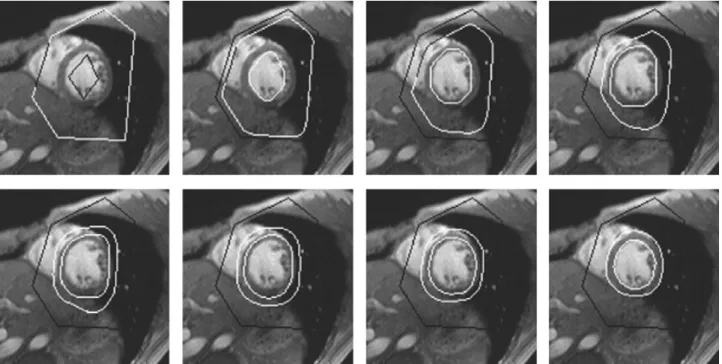
2.8 Whole heart segmentation result using deformable models [Peters et al., 2007]. . 39

2.9 Anatomical atlas-based segmentation. [Lorenzo-Vald´es et al., 2002]. . . 41

2.10 Temporal registration and resampling. [Lorenzo-Vald´es et al., 2004] . . . 41

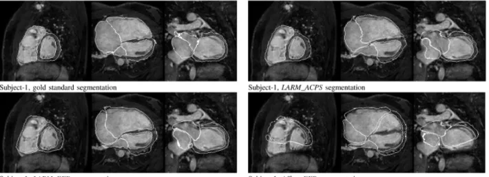
2.11 Comparison of manual segmentation, Affine+FFD, locally affine registration method (LARM)+FFD, and LARM+adaptive control point status (ACPS). [Zhuang et al., 2010]. . . 42

2.12 The general framework for multi-atlas based segmentation. . . 44

3.1 Example of contour tracking from [Remme et al., 2005]. . . 52

3.2 Overview of the temporal diffeomorphic free form deformations (TDFFD) framework. [De Craene et al., 2012] . . . 55

3.3 Example of HARP motion tracking. [Pan et al., 2005] . . . 57

3.4 Example of motion tracking using deformable models. [Haber et al., 2000] . . . . 61

4.1 Overall workflow of the segmentation framework. . . 70

4.2 Positive (green) and negative (red) examples from the training set for the cardiac detector. . . 71

4.3 Some examples of the results from the cardiac detector. . . 72

4.4 Example of the constructed probabilistic atlas. . . 75

4.5 Workflow of the multi-component EM estimation based segmentation component. 76

(25)

LIST OF FIGURES xxiii 4.7 The histogram of the Jacobian determinant and fitted Rician distribution from

different subjects. . . 82

4.8 The example images from different pathological groups. . . 85

4.9 Myocardial segmentation and registration uncertainties. . . 86

5.1 Multiple image acquisitions for cardiac motion tracking.. . . 91

5.2 Workflow of the proposed comprehensive cardiac motion method. . . 92

5.3 Spatial alignment of different images. . . 95

5.4 Removal of tags from 3D tagged MR. . . 97

5.5 The spatial weight map for the comprehensive motion tracking. . . 103

5.6 Automatic detection of valve points. . . 104

5.7 The parcellation of the endocardial surface into 16 segments. . . 108

5.8 This figure shows the relative landmark error in % when comparing the results of manual tag tracking with the registration-based motion tracking. . . 110

5.9 This figure shows the relative landmark error in % when comparing the results of manual tag tracking with registration-based motion tracking. . . 111

5.10 This figure shows the relative surface distance when comparing the result of an automatic segmentation with a manual segmentation. . . 112

5.11 This figure shows the manual landmark identification and distribution of the landmarks. . . 113

5.12 This figure shows the radial motion estimated from different methods. . . 114

5.13 This figure shows the longitudinal motion estimated from different methods. . . 114

5.14 This figure shows the circumferential motion estimated from different methods. . 115

(26)

5.16 A visualisation of the myocardial motion field in radial, longitudinal and circumferential directions. . . 116

6.1 Sparse representations of FFDs. . . 122

6.2 Visual comparison between the classic FFDs and the proposed SFFD using the colour scheme from [Baker et al., 2007]. . . 125

6.3 The accuracy of different parameters. . . 130

6.4 The effect of the sparsity parameter. . . 130

7.1 This figure shows the graphs for SDI. . . 140

7.2 Acute response and remodelling against volume and muscle thickening SDI. [Duckett et al., 2012] . . . 141

7.3 Acute response and remodelling against strain SDIs. [Duckett et al., 2012] . . . 142

7.4 Flow chart showing the main steps for co-registering and segmenting the cardiac MR images to obtain a 3D transformation between baseline and follow-up images.143 7.5 3D visualisation of different indices of the LV in an 51 year old male patient.

[Oregan et al., 2012] . . . 146

7.6 A Dot density histogram for each variable derived from the image registration model at baseline and follow-up. [Oregan et al., 2012] . . . 147

(27)

Chapter 1 Introduction

This chapter gives an introduction to this thesis. Cardiovascular diseases (CVDs) is one of the major causes of death in the western world. In recent years, significant progress has been made in the care and treatment of patients with such diseases. A crucial factor in this progress has been the development ofmagnetic resonance (MR)imaging which makes it possible to diagnose and assess the cardiovascular function of the patient non-invasively. The ability to obtain high-resolution, cine volumetric images easily and safely has made it the preferred method for diagnosis of cardiovascular diseases. MR images is also unique in its ability to introduce noninvasive markers directly into the tissue being imaged (MR tagging) during the image acquisition process. With the development of advanced MR imaging acquisition technologies, 3D MR imaging is more and more clinically feasible. This recent development has allowed new potentially 3D image analysis technologies to be deployed. Quantitative analysis of the cardiovascular system from the images remains a challenging topic.

1.1 Background and motivation

In this section, we review the basic anatomy and function of the heart and give a brief introduction of CVDs and the main MR imaging techniques that have been developed for diagnosing patients withCVDs. In addition, we describe some of the basic clinical parameters

(28)

2 Chapter 1. Introduction

which are widely used in the assessment of CVDs.

1.1.1 The anatomy and structure of the heart

The cardiovascular system [Bray, 1999,Katz, 2005] is comprised of the heart and blood vessels whose main function is to circulate blood around the body. They act as a transport system for delivering oxygen from the lungs and nutrients from the gastrointestinal tract to the cells of the body. The heart (Figure1.1) consists of two pumps lying side by side which pump in phase with each other. Each pump has an atrium and a ventricle as shown in the figure. The right atrium receives venous blood from the body and passes it through into theright ventricle (RV) where it is pumped to the lungs (pulmonary circulation) for oxygenation. At the same time the left atrium receives oxygenated blood from the lungs and the left ventricle (LV) pumps it out to the rest of the body (systemic circulation).

Figure 1.1– The heart consists of two pumps lying side by side. The arrows show the direction of blood flow in the two sides. This figure has been adapted from Figure 13.3 in [Bray, 1999].

The four chambers of the heart are separated from each other and the rest of the body by four sets of valves. The bicuspid (or mitral) and tricuspid atrioventricular (AV)valves separate the left and right atria and ventricles respectively, while the aortic valve separates the LV from the aorta, and the pulmonary valve separates the RV from the pulmonary artery. Thin chords called the chordae tendineae are attached to the AV valves and projections of the ventricular

(29)

1.1. Background and motivation 3 muscles known as the papillary muscles. During ventricular contraction the papillary muscles tense and prevent the valves from inverting into the atrium.

The cardiac cycle

Venous blood returning to the heart from the rest of the body flows continuously from the superior and inferior vena cava into the right atrium, while oxygenated blood from the lungs enters the left atrium through the pulmonary veins. When the pressure in the atria exceeds the pressure in the ventricles, the AV valves open and the blood enters the ventricles. When the ventricles are about 80% full, the atria contract and propel more blood into the ventricles completing the ventricular filling. This stage of the cardiac cycle, when the ventricular filling takes place, is known as diastole.

After a very short pause (approx. 0.1 s), the ventricles contract. This stage is known as systole. As the ventricles contract the pressure in the ventricles increases rapidly and exceeds the atrial pressure, causing the AV valves to close. Simultaneously, the papillary muscles contract so that the AV valves do not revert back into the atria. The continued contraction raises the ventricular pressure beyond the pressure in the aorta and the pulmonary artery. This causes the pulmonary and aortic valves to open and blood is ejected at low pressure from the RVinto the pulmonary circuit and at high pressure from the LV into the systemic circuit. When the pressure in the ventricles falls below that in the pulmonary artery and the aorta, the pulmonary and aortic valves close. Similarly when the ventricular pressure falls below the atrial pressure, the AV valves open and the ventricles start to refill with blood again and the cycle repeats.

The electrical activation of the heart

The myocardium (the heart muscle) is comprised of muscle cells called myocytes. These are typically 10−20µm in diameter and 50−100µm in length. The junction between adjacent myocytes, called the intercalated disc, allows electrical impulses to be transmitted from cell to cell making the myocardium act like an electrically continuous sheet. The contraction of the

(30)

heart is initiated by the sino-atrial (SAt)node which acts as a pacemaker, dictating the rate of beating of the heart (Figure1.2). The node is composed of myocytes which generate an action potential roughly once every second that excites the adjacent atrial work cells and causes a wave of depolarisation to travel across the two atria and initiates atrial systole.

Figure 1.2– The cardiac conduction system adapted from figure 13.5 in [Bray, 1999].

The electrical impulse then reaches the AV node in the atrial septum (the wall separating the two atria). The impulse is delayed by the AV node allowing the atria to finish contracting before the ventricles are activated. The electrical impulse then travels down a narrow bundle of conduction fibers called the bundle of His, which separates into two parts, one activating the LV of the heart and the other in the RV. The bundle of His terminates in the Purkinje network, located in the subendocardium, which distributes the electrical impulse rapidly to the work cells of the myocardium.

The coronary circulation

The heart receives the energy it needs from the coronary circulation (Figure1.3), which consists of five main arteries: the left main coronary artery (LM), the right coronary artery (RCA), the left anterior descending artery (LAD), theleft circumflex artery (CIRC), and the posterior descending artery (PDA). TheRCAand theLMarise from the aorta, while theLADandCIRC arise from the LM when it splits into two. The PDA arises from the RCA in approximately 90% of the human population and from theCIRC in approximately 10% of the population.

(31)

1.1. Background and motivation 5

Figure 1.3– The coronary circulation. [Institute, 2010]

Type of CVD Deaths (in %) Coronary heart disease 49.9

Stroke 16.5

High blood pressure 7.5 Congestive heart failure 7.0 Diseases of the arteries 3.4

Other 15.6

Table 1.1– Percentage breakdown of deaths due to CVDs [Members et al., 2012].

The blood flow from the coronary arteries reaches the myocardium by vessels which penetrate the walls of the ventricles. This means that the endocardial regions of the heart are very vulnerable to cell death, or infarction, if coronary artery occlusion occurs. This is especially the case for the myocardium of the LV which has a much thicker wall than the RV. Occlusion of theLMis much more serious than occlusion of any one of the other arteries since this blocks off all of the blood supply to the myocardium of the LV.

1.1.2 Cardiovascular diseases

Table 1.1 shows a percentage breakdown of the deaths due to CVDs in the USA [Members et al., 2012]. In both the USA and Europe, the greatest proportion of deaths resulting from CVDs are due to coronary heart disease (CHD) [Members et al., 2012].

(32)

Coronary heart disease, acute coronary syndrome, and angina pectoris

Coronary heart disease is the narrowing or blockage of the coronary arteries, usually caused by atherosclerosis. Atherosclerosis is the buildup of cholesterol and fatty plaques on the inner walls of the arteries. These plaques can restrict blood flow to the heart muscle by physically clogging the artery or by causing abnormal artery tone and function. Without an adequate blood supply, the heart becomes starved of oxygen and the vital nutrients it needs to work properly. This can cause chest pain known as angina. If the blood supply to a portion of the heart muscle is cut off entirely, or if the energy demands of the heart become much greater than its blood supply, a heart attack may occur.

Acute coronary syndrome (ACS)refers to any group of symptoms attributed to the obstruction of the coronary arteries. The most common symptom prompting diagnosis ofACSis chest pain, often radiating to the left arm or angle of the jaw, pressure-like in character, and associated with nausea and sweating. Acute coronary syndrome usually occurs as a result of one of three problems: ST elevation myocardial infarction (30%), non ST elevation myocardial infarction (25%), or unstable angina (38%) [Torres and Moayedi, 2007]. Here the ST elevations refers to a finding of an electrocardiogram, wherein the trace in the ST segment is abnormally high above the isoelectric line. The ST segment corresponds to a period of ventricle systolic depolarisation, when the cardiac muscle is contracted.

Angina pectoris, commonly known as Angina, refers to chest pain due to ischemia of the heart muscle, generally caused by the obstruction or spasm of the coronary arteries. Coronary artery disease, the main cause of angina, is due to atherosclerosis of the cardiac arteries. Angina occurs when there is an imbalance between the heart’s oxygen demand and supply. This imbalance can result from an increase in demand (e.g. during exercise) without a proportional increase in supply. When the symptoms of coronary occlusive disease do not change the patient is said to have stable angina pectoris. Stable angina often decreases in severity over weeks and months because of the development of collateral vessels and enlargement of partially occluded coronary arteries.

(33)

1.1. Background and motivation 7 Stroke (cerebrovascular disease)

Stroke is one of theCVDs, which affects the arteries leading to and within the brain. A stroke occurs when a blood vessel carrying oxygen and nutrients to a part of the brain is blocked by a clot, or ruptures. As a result, the affected area of the brain cannot function, which might result in an inability to move one or more limbs on one side of the body, inability to understand or formulate speech, or an inability to see one part of the visual field. The part of the brain affected can be damaged because of the lack of blood flow and the consequences can be devastating. The patient may become paralysed in addition to the loss of language skills and vision. Stroke can be treated, if the warning signs are detected early enough, by drugs or surgical intervention.

High blood pressure

High blood pressure, is often called the ”silent killer” as no symptoms are shown in a person suffering from thisCVDs. Untreated it can lead to stroke, heart attack, heart failure, or kidney failure. Medications are available which can help to reduce and control high blood pressure but it is a lifelong disease, which cannot be cured. It may also lead to hypertensive heart disease. Systemic hypertension is one of the most prevalent and serious causes of coronary artery and myocardial disease in the United States [Rubin and Reisner, 2009]. Chronic hypertension leads to pressure overload and results first in compensatory left ventricular hypertrophy and, eventually, cardiac failure.

Congenital cardiovascular defects

Congenital cardiovascular defects (CCD), also known as congenital heart defects, are structural problems that arise from abnormal formation of the heart or major blood vessels. Significant congenital cardiovascular defects occur in almost 1% of all live births. The International statistical classification of diseases and related health problems (ICD-9)1 _{lists 25 congenital}

(34)

heart defects codes, of which 21 designate specified anatomic or hemodynamic lesions [Members et al., 2012].

Defects range in severity from tiny pinholes between chambers that may resolve spontaneously, to major malformations that can require multiple surgical procedures before school age and may result in death in utero, in infancy, or in childhood. Common complex defects include the following [Members et al., 2012,Rubin and Reisner, 2009]:

• Tetralogy of fallot (TOF) represents 10% of all cases of CCD and is the most common cyanotic heart disease in older children and adults. It involves four heart malformations: e.g. infundibular pulmonary stenosis, overriding aorta, ventricular septal defect and right ventricular hypertrophy.

• AV septal defects are caused by an abnormal or inadequate fusion of the superior and inferior endocardial cushions with the mid portion of the atrial septum and the muscular portion of the ventricular septum.

• Coarctation of the aorta is a local constriction that almost always occurs immediately below the origin of the left subclavian artery at the site of the ductus arteriosus.

• Hypoplastic left heart syndrome is aCCDin which the left ventricle of the heart is severely underdeveloped. If part of the endocardial tube gets pinched shut in a region that becomes the future ventricle, hypoplastic heart syndrome will occur. If the pinched part of the endocardial tube is the bulbus-cordis region of the developing heart, hypoplastic right syndrome will occur. If it is in the ventricle region, it will be on the left side that is hypoplastic.

Congenital heart defects are serious and common conditions that have a significant impact on morbidity, mortality, and health care costs for children and adults.

(35)

1.1. Background and motivation 9 Cardiomyopathy and heart failure

Because of the heart’s capacity to compensate, congestive heart failure is often tolerated for years. The heart’s ability to adapt to injury is based on the same mechanisms that allow cardiac output to increase in response to stress. The fundamental compensatory mechanism is the Frank-Starling mechanism [Rubin and Reisner, 2009]: the cardiac stroke volume is a function of diastolic fiber length. Within certain limits, a normal heart will pump whatever volume is brought to it by the venous circulations. Stroke volume, a measure of ventricular function, is enhanced by increasing ventricular end diastolic (ED) volume secondary to an increase in atrial filling pressure.

Anything that increases cardiac workload for a prolonged period or produces structural damage may eventually lead to myocardial failure. Ischemic heart disease is by far the most common condition responsible for cardiac failure, accounting for 87% of strokes from heart disease [Members et al., 2012]. Most of the remaining cases are caused by nonischemic forms of heart muscle disease and congenital heart disease. Ventricular hypertrophy is observed in virtually all conditions associated with chronic heart failure.

Cardiac dysrhythmias

Cardiac dysrhythmias refer to any variation from the normal rate or rhythm (which may include the origin of the impulse and/or its subsequent propagation) in the heart. The heartbeat may be too fast or too slow, and may be regular or irregular. A heart beat that is too fast is called tachycardia and a heart beat that is too slow is called bradycardia.

It can be classified into the following forms according to ICD-9:

• Paroxysmal supraventricular tachycardia: An episodic form of supraventricular tachycar-dia, with abrupt onset and termination.

• Paroxysmal ventricular tachycardia: A tachycardia arising distal to bundle of His, with a rate greater than 100 beats per minute.

(36)

• Atrial fibrillation: An arrhythmia in which minute areas of the atrial myocardium are in various uncoordinated stages of depolarisation and repolarisation; instead of intermittently contracting, the atria quiver continuously in a chaotic pattern, causing a totally irregular, often rapid ventricular rate.

• Atrial flutter: An electrocardiographic finding of an organised rhythmic contraction of the atria, generally at a rate of 200-300 beats per minute.

• Ventricular fibrillation: An arrhythmia characterised by an irregular pattern of high or low-amplitude waves that cannot be differentiated into QRS complexes or T waves. These electrocardiographic waves occur as a result of fibrillary contractions of the ventricular muscle due to rapid repetitive excitation of myocardial fibers without coordinated contraction of the ventricle.

• Ventricular flutter: A ventricular tachyrhythmia characterised electrocardiographically by smooth undulating waves with QRS complexes merged with T waves, a rate of approximately 250 per minute.

• Cardiac arrest: Sudden cessation of the pumping function of the heart, with disappearance of arterial blood pressure, connoting either ventricular fibrillation or ventricular standstill.

• Sinoatrial node dysfunction: A derangement in the normal functioning of the sinoatrial node. Typically, SAtnode dysfunction is manifest as sinoatrial exit block or sinus arrest, but may present as an absolute or relative bradycardia in the presence of a stressor. It may be associated with bradycardia-tachycardia syndrome.

• Other specified and unspecified cardiac dysrhythmias.

The most common symptom of arrhythmia is an abnormal awareness of the heartbeat, called palpitations. These may be infrequent, frequent, or continuous. Some of these arrhythmias are harmless (though distracting for patients) but many of them predispose to adverse outcomes. Some arrhythmias do not cause symptoms and are not associated with increased mortality. However, some asymptomatic arrhythmias are associated with adverse events. Examples

(37)

1.1. Background and motivation 11 include a higher risk of blood clotting within the heart and a higher risk of insufficient blood being transported to the heart because of weak heartbeat. Other increased risks are of embolisation and stroke, heart failure and sudden cardiac death. Medical assessment of the abnormality using an electrocardiogram is the most common way to diagnose and assess the risk of any given arrhythmia.

1.1.3 Cardiac dyssynchrony, remodelling and resynchronisation

ther-apy

Patients with dilated cardiomyopathy (DCM) that is further complicated by intra-ventricular conduction delay with dyssynchronous wall motion have an increased mortality risk as compared to the general DCM population. Dyssynchrony reduces cardiac systolic function while increasing oxygen consumption, and may be a source of arrhythmia [Kass, 2002]. The recent development of endocardial lead systems to activate the left ventricle prematurely has yielded the novel therapeutic option of resynchronisation therapy to correct cardiac dyssynchrony. Using either biventricular or left ventricular pre-excitation, systolic function and energetic efficiency can be substantially enhanced in heart failure patients who have underlying discoordinate contraction.

Left ventricular remodelling is the process by which ventricular size, shape, and function are regulated by mechanical, neurohormonal, and genetic factors [Pfeffer and Braunwald, 1990,

Sutton and Sharpe, 2000]. Remodelling may be physiological and adaptive during normal growth or pathological due to myocardial infarction, cardiomyopathy, hypertension, or valvular heart disease. Postinfarction remodelling has been arbitrarily divided into an early phase (within 72 hours) and a late phase (beyond 72 hours) [Pfeffer and Braunwald, 1990]. The early phase involves expansion of the infarct zone, which may result in early ventricular rupture or aneurysm formation. Late remodelling involves the left ventricle globally and is associated with time-dependent dilatation, the distortion of ventricular shape, and mural hypertrophy. The failure to normalise increased wall stresses results in progressive dilatation, recruitment of border zone myocardium into the scar, and deterioration in contractile function [Sutton and

(38)

Sharpe, 2000].

On the other hand, a reduction in LV end-systolic volume (ESV) of 10% signifies clinically relevant reverse remodelling, which is a strong predictor of lower long-term mortality and heart failure events [Yu et al., 2005]. [Yu et al., 2005] suggests that assessing volumetric changes after an intervention in patients with heart failure provides information predictive of natural history outcomes.

[Bax et al., 2004] found a interesting relationship between cardiac dyssynchrony and cardiac resynchronization therapy (CRT):

• The LV dyssynchrony is larger in responders then non-responders to CRT;

• baseline LV dyssynchrony of 65 ms or more has a sensitivity and specificity of 80% to predict clinical response and 92% to predict reverse LV remodelling;

• patients with extensive dyssynchrony who undergo CRT have an excellent prognosis (6% event rate), whereas patients who do not have dyssynchrony and undergo CRT have a poor prognosis (event rate 50

This leads to the conclusion that patients with extensive LV dyssynchrony respond well to CRT. Using a cutoff level of 65 ms, a sensitivity and specificity of 80% were obtained for predicting clinical response of reverse remodelling and 92% for predicting reverse LV remodelling. Moreover, patients with LV dyssynchrony of approximate 65 ms had an excellent prognosis after CRT, in contrast to patients with < 65 ms who had a high event rate (50%) during one-year follow-up.

1.1.4 Cardiac magnetic resonance imaging

Common cardiac imaging techniques include echocardiogram (US), positron emission tomog-raphy (PET), computed tomography (CT) and single-photon emission computed tomography (SPECT). An echocardiogram uses ultrasonic waves for real-time visualisation of the heart

(39)

1.1. Background and motivation 13 chamber and blood flow. Recently, it has become one of the most commonly used tools in the diagnosis of heart problems, as it allows non-invasive, low-cost visualisation of the heart. In addition the blood flow in the heart can be visualised using a technique known as Doppler US. CT is an imaging methodology which uses X-rays to produce tomographic images of the body. This is achieved by reconstructing a tomographic image from a large series of two-dimensional X-ray images taken around a single axis of rotation. WhileCT offers high spatial and temporal resolution, it requires a significant amount of radiation to produce good quality images. PET is an imaging methodology based on positron emitting radioisotopes. It enables visual analysis of multiple different metabolic processes (e.g. glucose uptake) and is thus one of the most flexible functional imaging technologies. However, it only offers low spatial and temporal resolution and can only be carried out in specialised centres. SPECT is similar to PET in its use of radioactive tracer material and detection of gamma rays. Cardiac gated acquisitions are possible with SPECT, however, the image quality is often inferior to that of PETimaging.

The work in this thesis focuses on MR imaging [Lauterbur, 1973] which is primarily a medical imaging technique most commonly used in radiology to visualise the anatomy and function of the body. MR imaging provides a much greater contrast between the different soft tissues of the body compared to CT, making it especially useful in neurological (brain), musculoskeletal, cardiovascular, and oncological (cancer) imaging. UnlikeCT, it does not use ionising radiation, but a powerful magnetic field to align the magnetisation of (usually) hydrogen atoms in water or fat in the body. Radio frequency (RF)fields are used to systematically alter the alignment of this magnetisation, causing the hydrogen nuclei to produce a rotating magnetic field detectable by the scanner. This signal can be manipulated by additional magnetic fields to build up enough information to construct a tomographic image of the body.

Imaging planes

As the heart is continuously in motion, it is difficult to acquire a volume. Instead, we have to acquire slices. In this case, it is necessary to acquire images in multiple orientations so that an

(40)

accurate diagnosis can be made. It is common to define, orient, and display the heart using the long-axis (LA) of the left ventricle and selected planes at 90 degree angles relative to the LA. The commonly used imaging planes are shown in Figure 1.4 and some example images are shown in Figure 1.5. Other factors which also make cardiac magnetic resonance (CMR) imaging challenging are patient motion, respiration, and the anisotropic resolution of the images acquired. Typically, the in-plane resolution (1-2.5mm) is much higher than the through-plane resolution (8-10mm) as shown in Figure 1.6.

Figure 1.4 – The typical orientation ofCMR imaging planes [Heller et al., 2002]

Figure 1.5– The images from left to right show respectivelySA, horizontal long-axis and vertical long-axis views of the heart.

(41)

Figure 1.6 – This figure shows a simulated LA view of the heart which has been obtained by stacking a set ofSA images. As can be seen the through-plane resolution is much lower than the in-plane resolution.

Cine steady state free precession (cine MR imaging)

Images of the heart may be acquired in real-time with CMR, but the image quality is limited. Instead, most sequences useelectrocardiography (ECG)gating to acquire images at each phase of the cardiac cycle by accumulating information over several heart beats with breath holding. However, the breath holding introduces respiratory motion between slices acquired during different breath holds. Nevertheless, this technique forms the basis of functional assessment by CMR. Blood typically appears bright in these sequences due to its contrast properties and rapid flow. The technique can discriminate very well between blood and myocardium. The most frequently usedMRacquisition sequence for this is called balanced steady state free precession (bSSFP) [Carr, 1958]. SA, four (4CH or horizontal long-axis (HLA)), three (3CH) and two chamber (2CH or vertical long-axis (VLA)) views are often acquired during a routine clinical setting. An example of this image modality is given in Figure 1.7.

Spatial modulation of magnetisation imaging (tagged MR imaging)

Myocardial tissue in the body can be labelled by altering its magnetisation properties which are persistent even in the presence of motion. By measuring the motion of the labelled tissue, deformation fields in the myocardium can be reconstructed. Magnetic resonance tagging was first proposed in [Zerhouni et al., 1988]. [Axel and Dougherty, 1989b,Axel and Dougherty, 1989a] used aspatial modulation of magnetisation imaging (SPAMM) technique as a means of non-invasively introducing markers within the myocardium of the LV. The technique relies on the perturbation of the magnetisation in the myocardium by using a sequence of RF

(42)

saturation pulses before the acquisition of images using conventional MR imaging. Because the myocardium retains knowledge of the perturbation in the magnetisation the motion of the myocardium can be tracked during systole. To capture complex 3D cardiac motion patterns, multiple 2D tagged slices are usually acquired in different orientations. SPAMMhas been later extended tocomplementary spatial modulation of magnetisation imaging (CSPAMM) [Fischer et al., 1993] which separates the component of the magnetisation with the tagging information from the relaxed component by the subtraction of two measurements with first a positive and then a negative tagging grid. This technique improves the grid contrast and greatly facilitates the automatic evaluation of the myocardial motion. Thus the motion assessment of the heart throughout the entire cardiac cycle becomes possible. Recent reviews of MRtagging are given in [Axel et al., 2005].

Despite the advantage of the tagged imaging, a common difficulty to estimate cardiac motion from tagged images arises from the inevitable fading of the tag during the cardiac cycle. Tags which will survive the fading are usually manually segmented or identified in the last phase of the sequence of tagged images. Another difficulty is low temporal resolution: a sufficiently large motion will lead to misalignment between material points due to a lack of information between the tags.

3D tagged MR imaging

3D tagging has recently been implemented using three sequentially acquired 3D data sets with line tag preparation in each of the three spatial dimensions [Rutz et al., 2008]. Conventional 2D CSPAMM approaches are prone to slice misregistration and associated with long acquisition times. In the 3D tagging approach, a fast method for acquiring 3D CSPAMM data has been proposed. This 3D tagging method allows measuring the deformation of the whole heart in three breath-holds with a duration of 18 heartbeats each. Three acquisitions are sequentially performed with line tag preparations in each orthogonal direction. An example of this image modality is given in Figure 1.8.

(43)

Figure 1.7 – Example cine SSFP and LGE images from a volunteer. SSFP = Steady State Free Precession; LGE = Late Gadolinium Enhancement.

Late gadolinium enhancement MR imaging

Late gadolinium enhancement (LGE) MR imaging was introduced by [Saeed et al., 1989,Kim et al., 1996,McCrohon et al., 2003], to identify infarcted myocardial tissue using CMR. This technique incorporates the administration of relatively inert extracellular gadolinium contrast during gradient-echo inversion recovery imaging. In this image acquisition, areas of noninfarcted

(44)

Figure 1.8– Example whole heart TFE and tagged MR images from a volunteer. TFE = Turbo Field Echo; 3D tMR = 3D Tagged Magnetic Resonance Imaging.

tissue appear dark, and infarcted or fibrotic tissue appears bright, because of reduced clearance and increased volume of distribution of the gadolinium [Saeed et al., 1989]. This fundamental aspect of delayed enhancement MR has led to the expression: ”bright is dead.” [Mandapaka et al., 2006]. An example of this image modality is given in Figure 1.7.

(45)

1.1. Background and motivation 19 Whole heart Turbo Field Echo

The whole heart turbo field echo (TFE) sequence acquires an isotropic non-angulated volume [Uribe et al., 2007]. Images were acquired during free breathing with respiratory gating and at end-diastole with ECG gating. Different from previous acquisitions that were limited to 2D imaging, the isotropic 3D resolution enables the assessment of cardiac anatomy and function with minimum planning or patient cooperation. The respiratory self-gating technique is shown to improve image quality in free-breathing scanning. The resulting image gives a consistent single-phase high resolution image of the whole-heart anatomy. It can be treated as a baseline to align other image modalities into a common space [Zhuang et al., 2011], or to segment the whole-heart anatomy [Zhuang et al., 2008]. An example of this image modality is given in Figure1.8.

1.1.5 Indices of cardiac function

Functional indices are used clinically to assess and characterise cardiac function. Indices can be classed into two different categories: global and local indices. Global measures of cardiac function describe the overall ability of the heart to deliver blood to the rest of the body, while local functional indices are used to assess regional dysfunction in the heart, which is determined by the state of the myocardial tissue.

Global indices

Global indices assess the overall performance of the ventricles in their ability to eject blood. The left ventricular volume (LVV), left ventricular mass (LVM), stroke volume (SV), ejection fraction (EF) and cardiac output (CO) have all been used to assess the performance of the LV [Frangi et al., 2001].

LVV is defined as the volume enclosed by the LV. Volume-time curves of the left-ventricular cavity can provide information about the global contractility of the myocardium.

(46)

LVM is the mass of the LV and is equal to the volume of the myocardium, Vm, multiplied by

the density of the myocardium,ρm= 1.05g/cm3 [Foppa et al., 2005]:

LV M =Vmρm (1.1)

SV is defined as the volume ejected during systole and is equal to the difference between the end-diastolic volume (EDV) and theESV:

SV =EDV −ESV (1.2)

EF is defined as the ratio of the SV to the EDV:

EF = SV

EDV ×100% (1.3)

CO is the amount of blood ejected from theLV per minute and is equal to theSV multiplied by the heart rate (HR):

CO =SV ×HR (1.4)

Although global indices can be used to identify the abnormal functioning of the heart they do not indicate which regions of the heart have reduced contractile function. Moreover, for some patients, global indices fall within normal limits even though the wall motion may be abnormal. For example, patients suffering from hypertensive left ventricular hypertrophy may have normalEFwhile circumferential and longitudinal shortening are depressed [Kramer et al., 1994]. Measuring local indices can help to detect areas of the myocardium which have been damaged because of reduced blood flow.

Local indices

A widely recognised regional analysis technique for left ventricle myocardium is to use the 17-segment division model suggested by [Heller et al., 2002]. The motion of the heart can

(47)

1.1. Background and motivation 21 be characterised in terms of its contraction in the radial, circumferential and longitudinal directions. The regional wall motion (RWM), regional wall thickening (RWN) and regional myocardial strain (RMSt) in different directions are the local indices. These indices are often used to identify the abnormality.

Figure 1.9 – Bull-eye plot of the 17 segments of the left ventricular myocardium suggested by [Heller et al., 2002], Left the bull-eye plot, Right the anatomy landmarks for the bull-eye plot segments

RWM is defined as the myocardial movement of each segment. The functional abnormality of myocardium affects its contraction movement. It may, as a result, affect the total movement of a segment. Regional wall motion provides an indication of how healthy a specific segment is. In clinical practice, visual assessment by an experienced cardiologist is normally used to score the index as a semi-quantitative evaluation [Cigarroa et al., 1993]. For automatic assessment, the average radial distance from the myocardial region to the central axis is defined as the RWM:

RW M = (δES−δED)/δED×100% (1.5)

Here, δ is the radial distance from a myocardial point in one segment to the central axis of the blood cavity; ES is end-systolic; ED denotes end-diastolic.

(48)

RWN is a measure related to the thickness of myocardium at different phases. It provides an alternative to RWM and can be more sensitive in discriminating between passive motion and active motion. The index can be manually scored [Cigarroa et al., 1993] or automatically quantified by the following equation:

RW N = (ηES−ηED)/ηED×100% (1.6)

Here η is the thickness of the myocardium in a local region, defined as the distance between the endocardial and epicardial surfaces.

RMStis the fractional change of the length from a reference state to a subsequent state in the radial, circumferential and longitudinal directions. RMStis now considered the superior index to RWM and RWN in discriminating infarcted myocardium from ischemic one [G¨otte et al., 2001]. RMStin the different directions can be defined in terms of the off-diagonal terms of the Lagrangian strain tensor [Amini and Prince, 2001].

1.2 Objectives and challenges

It is now clear that MR imaging is becoming the modality of choice for cardiovascular image analysis as it has a number of advantages over other imaging techniques. It is safe, noninvasive and flexible. 2D, 3D and 4D images with high spatial and temporal resolution of the anatomy and physiology of the heart can be acquired in arbitrary orientations. Additionally,MRtagging can be used to measure detailed information about the myocardial deformation. However, there are a few technical challenges which need to be addressed.

Firstly, the ability to segment the images with pathological changes is necessary to gain a better understanding of the remodelling process of the heart following infarction. For example, determining the evolution of left ventricular remodelling and the relative contribution made by infarcted and remote myocardium to chamber dilatation has importance for evaluating interventions aimed at preventing heart failure. However, most existing cardiac image

(49)

1.3. Contributions 23 segmentation algorithms do not explicitly address subjects with pathological changes in the MR images caused by myocardial infarction, e.g. large shape variation and local varying levels of signal contrast. The contrast of the myocardial can be different in MR images due to infarction due to different tissue property between normal and infarcted myocardium. The consequence is that measuring remodelling following infarction is difficult or inaccurate using automated image segmentation techniques.

Secondly, differentMRacquisitions, includingSAandLAcineMRimages, 3DTFE MRimages and 3D tagged MR images, are often treated independently during the subsequent analysis of cardiac function. The global and local cardiac functional parameters may not be available from one acquisition and may differ across different acquisitions. For example, regional volume change over the cardiac cycle can be captured from SAandLA cineMRimages. However, this does not take into account the difference between active and passive motion. Potential ways of taking into account active myocardial motion are to use muscle thickening or strain. The strain index can only be fully extracted from a combination of different modalities.

Finally, most existing cardiac registration algorithms do not explicitly address the fact that the motion of different organs maybe different. This can lead to motion discontinuities in the image domain. For example, in the case of the heart, a sliding motion occurs at the pericardium. It is challenging to develop a motion tracking algorithm that can adaptively adjust to these motion discontinuities.

1.3 Contributions

The focus of the research presented in this thesis is the integrated use of multiple MR image acquisitions for cardiac function analysis. The work presented in this thesis makes three main technical contributions to the analysis of cardiac function in the context of segmentation and motion tracking. We also show two clinical applications that highlight the potential use of the developed techniques. The main contributions of the thesis are contained in chapters 4-7:

(50)

• A fully automatic cardiac segmentation technique is developed. The proposed segmenta-tion technique is capable of generating an accurate 3D segmentasegmenta-tion from multiple MR image acquisitions. To identify the cardiac anatomy from multiple image sequences, a spatial correction step is performed before segmentation. A 3D atlas is propagated to the SA and LA images using a single transformation across multiple acquisitions. A locally affine registration method (LARM) is used to cope with the large anatomical shape variations. Amultiple component expectation maximisation (MCEM) is employed to compensate for locally varying intensity contrast. Finally, 4D graph-cuts segmentation is used to extract the cardiac anatomy within each image acquisition consistently.

• A novel technique for myocardial motion estimation using both untagged and 3D tagged MR images is proposed. The novel aspect of our technique is in its simultaneous use of complementary information from both untagged and 3D tagged MRimages. To estimate the motion within the myocardium, we register a sequence of tagged and untagged MR images during the cardiac cycle to a set of reference tagged and untagged MR images at end-diastole. The similarity measure is spatially weighted to maximise the utility of information from both images. In addition, the proposed approach integrates a valve plane tracker and adaptive incompressibility into the motion tracking framework.

• A sparse representation for cardiac motion tracking usingfree-form deformations (FFDs) based on the principles of compressed sensing is proposed. The sparse free-form deformation (SFFD) model can capture fine local details such as motion discontinuities without sacrificing robustness. We demonstrate the capabilities of the proposed framework to accurately estimate smooth as well as discontinuous deformations in 2D and 3D image sequences. Compared to the classic FFD motion tracking approach, a significant increase in registration accuracy can be observed, in particular for images which exhibit discontinuous motion.

• Finally, two clinical applications for the above techniques are presented. We developed a framework which uses measures of myocardial motion to predict the response of individual patients to CRT. We also demonstrate the feasibility of using 3D probabilistic cardiac

(51)

1.4. Overview of thesis 25 atlases together with image registration to map the anatomical changes that occur over time in response to acute ST-elevation myocardial infarction (STEMI).

A list of publication arising from the work in this thesis can be found in AppendixA.

1.4 Overview of thesis

In this thesis, following this chapter, we review the current state-of-the-art for segmentation (Chapter 2) and motion tracking (Chapter 3) methods for cardiac MR images. The methods and algorithms that have been developed during our research are presented in the subsequent chapters. In Chapter 4 we develop a method for cardiac anatomy segmentation using atlas-based methods. In Chapter5a comprehensive cardiac motion tracking framework using tagged and untagged MR images is developed. In Chapter 6 we extend the classic non=rigid image registration with free-form deformations to a sparse representation. In Chapter 7 two clinical research applications that can be addressed by the techniques proposed in the thesis are presented.

Finally, in Chapter8, we summarise the work presented in this thesis and discuss future work.

1.5 Statement of originality

The material in this thesis has not previously been submitted for a degree at any university, and to the best of my knowledge contains no material previously published or written by another person except where due acknowledgement is made in the thesis itself.

(52)

Chapter 2 Cardiac image segmentation

In this chapter, we review several automatic and semi-automatic segmentation methods for CMR images. The remainder of the chapter is organised as follows: The challenge of the cardiac segmentation is presented in Section 2.1. In Section 2.2, a selection of current cardiac segmentation methods are categorised. In Section 2.3, recent popular methods in medical image segmentation, especially multi-atlas and patch-based segmentation, are discussed. In Section2.4, we discuss the development of evaluation techniques and benchmarks. Finally, the conclusions regarding the state-of-the-art are summarised in Section 2.5.

2.1 Challenge of cardiac segmentation

Most research effort in cardiac image segmentation has focused on the LV. This is largely due to the fact that the function of the RV is often less studied than that of the LV in CVDs. In addition, the LV is often easier to be identified and delineated than the RV: It has a well-defined ellipsoidal shape and is surrounded by the myocardium with a typical thickness of 6mm to 16mm [Petitjean and Dacher, 2011]. In contrast, the RV has a more complex crescent-like shape. The wall is also three to six times thinner than that of theLV, reaching the limit of the spatial resolution of MR imaging [Petitjean and Dacher, 2011].

The most common image obtained during a typicalCMRacquisition is theSAcineMRimages

(53)

2.1. Challenge of cardiac segmentation 27 (shown in Figure 1.7). The most frequently used MR acquisition technique for this is called bSSFP (as discussed in the introduction). A typical SA cine MR acquisition covers the whole heart with about 8-10 slices of an in-plane resolution of 1-2mm and through plane resolution of 8-10mm. Each slice is acquired in a separate breath-hold of the patient. About thirty cardiac phases can be obtained during one cardiac cycle depending on the heart rate.

Figure 2.1 – Variability among cardiac images. The image of the heart varies in terms of both intensity and shape. [Petitjean and Dacher, 2011]

One of the challenges for cardiac segmentation algorithms is that, as shown in Figure2.1,CMR images exhibit a great variability, both in terms of appearance and shape. The appearance may differ due to the use of the different MRscanners or differences in the acquisition protocols. It can also be caused by partial volume (PV) effects due to the non-zero thickness ofMR images slices: In some areas, a voxel can contain a mixture of several tissue types. Finally, pathological changes like infarction may cause local varying intensity contrast [Shi et al., 2011]. In terms of the shape, the ventricle can vary significantly across subjects, across different pathologies (dilation or hypotrophy), across time (before and after remodelling) and along the LA. This variability must be accounted for during the segmentation.

(54)

28 Chapter 2. Cardiac image segmentation

Figure 2.2 – A ROI identifying the heart and anatomy for SA cine MR images [Petitjean and Dacher, 2011]

epicardial wall consists of the boundary between the myocardium and the surrounding tissues. Some of the surrounding tissues show poor contrast compared to the myocardium. The segmentation is thus difficult. In contrast to this, MR images usually provide quite good contrast between the myocardium and the blood pool. This means that the endocardial wall is easier to be identified. However, intensity inhomogeneity caused by blood flow artifacts can make the segmentation challenging. In addition, the papillary muscles and trabecular inside the heart chambers have the same intensity as the myocardium. Thus it is often difficult to distinguish them from the myocardium. In most clinical segmentation protocols, the papillary muscles and trabecular should not be taken into account for the delineation of the endocardial wall.

Figure 2.3 – Variability of the heart in SA MR images along the LA. [Petitjean and Dacher, 2011]

(55)

2.1. Challenge of cardiac segmentation 29 Another major challenge in the segmentation ofSAcineMRimages is the large variability along the LA as shown in Figure 2.3. The apical and basal slices are more difficult to be segmented than mid-ventricular ones. Small structures at the apex are usually degraded due to the large through plane resolution. On the other hand, the shape of the LV varies often drastically in slices close to the base of the heart, because of the vicinity of the atria. In general, the RV shape varies even more along the LA.

Spatial misalignment is another challenge in the segmentation of SA cine MR images. Due to potential differences in the position of the heart during different breath-holds (e.g. due to respiration) there is usually some spatial misalignment between the images (inter-sequence misalignment) as well as between individual slices of the SA and LA images (intra-sequence misalignment). The image segmentation can be correct in 2D slices but distorted in 3D anatomical space and the distorted 3D segmentation can cause inconsistencies and inaccuracies in the final derived indices of cardiac function.

Several attempts have been made to segment the myocardium from 3D whole-heart images, include CT [Zheng et al., 2007] and 3D TFE MR images [Peters et al., 2007,Zhuang et al., 2010]. Compared toSAcineMRimages, 3D whole-heart images are limited in terms of clinical availability as well as in terms of temporal resolution. This limits the ability to compute clinical parameters like EFwhich require segmentation at theend systolic (ES) andED phases of the cardiac cycle. On the other hand, 3D whole-heart images provide nearly isotropic image resolution, which can increase segmentation accuracy on apical and basal segments and avoid the spatial misalignment problem.

The segmentation of the ventricles during the full cardiac cycle allows temporal volume and the mass changes to be assessed and is of great interest as an indicator of cardiac performance [Caudron et al., 2011]. However, because of the lack of landmarks inside the mycardium, the circumferential (twisting) and the longitudinal (through plane) myocardial motion cannot be analysed from SA cine MR images but requires dedicated modalities such as 2D or 3D tagged MR images [Chandrashekara et al., 2004,Rougon et al., 2005,Rutz et al., 2008].