Representation of complex spectrogram via phase conversion
Kohei Yatabe
, Yoshiki Masuyama
y, Tsubasa Kusano
zand Yasuhiro Oikawa
x Department of Intermedia Art and Science, Waseda University,3–4–1 Okubo, Shinjuku-ku, Tokyo, 169–8555 Japan
Abstract: As importance of the phase of complex spectrogram has been recognized widely, many techniques have been proposed for handling it. However, several definitions and terminologies for the same concept can be found in the literature, which has confused beginners. In this paper, two major definitions of the short-time Fourier transform and their phase conventions are summarized to alleviate such complication. A phase-aware signal-processing scheme based on phase conversion is also introduced with a set of executable MATLAB functions (https://doi.org/10/c3qb).
Keywords: Phase-aware signal processing, Short-time Fourier transform (STFT), Discrete Gabor transform (DGT), Phase conventions, Instantaneous frequency
PACS number:43.60.Hj, 43.60.Pt [doi:10.1250/ast.40.170]
1.
INTRODUCTION
Time-frequency analysis is an indispensable tool in audio signal processing. Among many including cosine and wavelet transform, the short-time Fourier transform (STFT), or discrete Gabor transform (DGT), is one of the most popular choices. A reason behind the popularity should be close connection to the well-understood Fourier transform whose magnitude is translation invariant (un-changed under translation in time domain). STFT inherits such invariance (or robustness) of the Fourier transform to some extent, which allows friendly design of a signal-processing algorithm acting on magnitude of STFT. The unfriendly part of STFT is concentrated intophasewhose (seemingly) fancy structure had forced ones to abandon it. Recently, as importance of phase has been recognized widely, phase-aware signal processing is receiving increas-ing attention from the society. A number of techniques has been introduced over the past few decades to manage information buried inside phase, and the latest concepts of the processing techniques are constructed upon them. However, several definitions and terminologeis for the same concept can be found in the literature, which has confused beginners.
In this paper, two major definitions of STFT (together with DGT) and their phase conventions are summarized. The instantaneous frequency and its calculation based on
the window function are also reviewed. Then, a signal processing scheme based on phase conversion [1] is explained with some related topics. A set of MATLAB functions for its calculation is available and can be downloaded1as a supporting material.
2.
STFT VS DGT
In the literature of audio signal processing, the term ‘‘STFT’’ is often utilized in place of what the literature of time-frequency analysis calls ‘‘DGT’’ (in honor of D. Gabor). In this section, their difference is contrasted by brief definitions and their inversion formulas.
2.1. Terminology in Time-frequency Analysis
For a fixed window function w6¼0, STFT of a time-domain signalxðtÞ with respect towðtÞis defined as
Xðf;tÞ ¼
Z Rx
ðÞwðtÞe2ifd; ð1Þ
wherezis the complex conjugate ofz, andi¼pffiffiffiffiffiffiffi1is the imaginary unit. In the case of a discrete signal x½n with indexn2Z, the discrete STFT is given by
X½m;n ¼X
lx½lw½lne
2iml=L; ð2Þ
where L is the length (total number of elements) of the signal. Note that, in this definition, the window w½n is translated sample-by-sample, i.e., STFT results in the fully-redundant time-frequency representation.
Obviously, such full redundancy is not necessary for
e-mail: [email protected] y
e-mail: [email protected] ze-mail: [email protected] x
e-mail: [email protected] 1Available at Code Ocean:https://doi.org/10/c3qb
INVITED REVIEW
representing a signal, and thus it is natural to consider reduction of the number of elements by downsampling. With step-size parameters a;b>0 and countable indices
n;m2Z, STFT in Eq. (1) can be downsampled as
X½m;n ¼
Z R
xðÞwðanÞe2ibmd; ð3Þ
which is called theGabor transform2. Its discrete counter-part with integer shifting stepsa;b2N,
X½m;n ¼X
lx½lw½lane
2ibml=L; ð4Þ
is the so-called DGT (discrete Gabor transform) [2–6]. The term ‘‘spectrogram’’ is also used differently in the literatures. In time-frequency analysis, the squared magni-tude of STFTjXðf;tÞj2 is only referred to as spectrogram. In this paper, it is used in wider sense as in the acoustics literature: DGT coefficient X½m;n is called complex spectrogram, while jX½m;nj and jX½m;nj2 are called magnitude (or amplitude) and power spectrograms, respec-tively.
2.2. Inversion Formula for STFT
One particularly nice property of STFT in Eq. (1) is that it admits the following inversion formula:
xðtÞ ¼ 1 hw; i
Z R2
Xwðf; ÞðtÞe2iftdfd; ð5Þ
where Xw is X with respect to windoww, is a window function satisfying hw; i 6¼0, and h;i is the standard inner product3. Similar inversion formula is also available for the discrete STFT in Eq. (2). Many signal processing methods rely on such inversion after modifying time-frequency-domain coefficients.
Unlike STFT, the Gabor transform and DGT do not admit such a simple inversion formula. In general, a pseudo-inverse of the transform is required to reconstruct the time-domain signal from its time-frequency represen-tation. Fortunately, the pseudo-inverse of Gabor-type transformations is highly structured, which allows an inversion algorithm requiring much less computation.
2.3. Inversion and Related Topics on DGT
Let DGT be explained with more details for the finite-dimensional settings. When considering finite samples of a signal, its boundary is always a source of trouble. A mathematically sound treatment for the inconvenience is to impose the periodic boundary condition,
x½lþL ¼x½l; ð6Þ
as usual (for, say, the discrete Fourier transform), which can be easily realized by the modulo operation. This treatment preserves important properties of essential operations including translation and convolution.
Some inconvenience arising from the periodicity is then eliminated by zero-padding4. For givena;b2N, the signal length L should be divisible so that there exist
N;M2N satisfying aN ¼bM¼L. This requirement can be fulfilled simply5 by increasing the length L via zero-padding untilLbecomes divisible with bothaandb. With these settings, DGT is defined as
X½m;n ¼X L1
l¼0
x½lw½lane2ibml=L; ð7Þ
wheren2 f0;. . .;N1g,m2 f0;. . .;M1g, andw zero-padded for extending its length to L is also treated periodically (index is read as½lanmodL).
Although inversion of DGT is not simple as STFT owing to its reduced redundancy, structure of the pseudo-inverse of DGT admits a similar inversion formula:
x½l ¼X N1 n¼0 X M1 m¼0 Xw½m;n½lane2ibml=L; ð8Þ
where is a dual window of w. While STFT can be inverted with almost any synthesis window, DGT can reconstruct the signal only when some appropriate syn-thesis window with respect to the analysis window w
is utilized6. All procedures for calculating an appropriate synthesis window and the above DGT can be found in the supplemental MATLAB codes (see the footnote in Sect. 1 for the download URL).
When DGT is redundant, there exist infinitely many dual windows corresponding to a single window w. Therefore, many attempts to design a dual window with some desirable properties have been made [8–11]. A window is calledtightwhen itself is proportional to its dual window, and its useful properties in signal processing have been studied [11–14]. These theories regarding the Gabor transform are based on frame theory [15] which also includes wavelet and general filterbanks [2–6].
3.
PHASE AND ITS DERIVATIVE
The complex argument of a time-frequency represen-tation is calledphase, while its (time) derivative is referred to as instantaneous frequency. Their definitions can vary
2The special case of Eq. (3) utilizing the Gaussian window and a¼b¼1was proposed by D. Gabor in 1946.
3
More precisely,x;w; 2L2ðRÞ, andh;iis the L2standard inner product. See, for example, [7] for rigorous statements.
4
The side effect of the periodic boundary condition appears only within the window function including the end point. Therefore, it can be eliminated by sufficiently large zero-padding when the window is compactly supported.
5Denoting the least common multiple ofaandbasc, suchLcan be found byL¼ dL~=cec, where L~ is the signal length before zero-padding, anddeis the ceiling function.
6
according to the definition of the corresponding transform, which is briefly summarized in this section.
3.1. Another Definition of STFT
The definitions in Sect. 2 are merely examples, and some other definitions are widely accepted. STFT in Eq. (1) handles the signal xðÞ and complex sinusoid
e2if through the same variable, and only the window
function wðtÞ is translated. That is, the signal and sinusoid share the time origin (t¼0), while that of the window is independent. Alternatively, the window can share the time origin with the sinusoid, which results in another definition of STFT:7 Xðf;tÞ ¼ Z Rx ðÞwðtÞe2ifðtÞd; ¼ Z Rx ðþtÞwðÞe2ifd; ð9Þ
where the relation between the signal and sinusoid is different from Eq. (1). Computing the fast Fourier trans-form (FFT) after truncating the signal by a compactly-supported window, which is a usual procedure in audio signal processing, corresponds to this definition8 as the time index of FFT is treated relatively to the window.
3.2. Phase Difference between Two STFTs
Since the complex sinusoid e2if in Eq. (1) can be extracted from that of Eq. (9) as
e2ifðtÞ¼e2ife2ift ¼e2ife2ift; ð10Þ
the relation between the spectrograms is given as
XEq(9)ðf;tÞ ¼e2iftXEq(1)ðf;tÞ; ð11Þ
where XEq(9)ðf;tÞ and XEq(1)ðf;tÞ represent Xðf;tÞ in
Eqs. (9) and (1), respectively. Therefore, their complex argumentsEq(9)ðf;tÞandEq(1)ðf;tÞ, or phases, are related
to each other in the following way:
Eq(9)ðf;tÞ ¼2ftþEq(1)ðf;tÞ: ð12Þ
This difference can be easily contrasted by considering
xðtÞ ¼e2it ð13Þ
as a signal. For simplicity, let the window functionw be nonnegative. STFT of Eq. (13) yields
XEq(1)ðf;tÞ ¼ Z
R
wðtÞe2iðfÞd ð14Þ
which becomes a real value at the frequency of the signal (f ¼) because e0 ¼1 andw is real. In other words, its
phase is zero and does not evolve along time at f ¼,
Eq(1)ð;tÞ ¼0: ð15Þ
On the other hand, in the same situation, phase rotates along time if STFT is defined as in Eq. (9):
Eq(9)ð;tÞ ¼2t; ð16Þ
where 2ambiguity of phase is ignored in this paper.
3.3. Instantaneous Frequency
Let a derivative of phase with respect to time, @=@t, be considered. It can be obtained as a part of the time derivative of Xðf;tÞ ¼Aðf;tÞeiðf;tÞ as9 @X @t ¼ @A @t e iþi A ei@ @t : ð17Þ
When A6¼0, dividing Eq. (17) by X¼Aei results in
ð@X=@tÞ=X¼ ð@A=@tÞ=Aþið@=@tÞ, and thus @ @t ¼Im @X @t 1 X ; ð18Þ
where Im½ denotes the imaginary part. This quantity is called instantaneous frequency and can be calculated if
@X=@t is available together withX.
One popular method to obtain the time derivative ofX
is STFT with a differentiated window dw=dt. Because
@X @t ðf;tÞ ¼ @ @t Z Rx ðÞwðtÞe2ifd; ¼ Z Rx ðÞdw dt ðtÞe 2ifd; ð19Þ
calculating STFT with dw=dt yields @X=@t. Therefore, after calculating the time derivative of a window, the instantaneous frequency can be retrieved through Eq. (18) with two STFTs usingwanddw=dt.
3.4. Difference of Instantaneous Frequencies between Two STFTs
Since phase depends on the definition of STFT as in Sect. 3.2, the instantaneous frequency also differs in accordance with it. The relation between the instantaneous frequencies calculated via Eqs. (9) and (1) is
@Eq(9)
@t ðf;tÞ ¼2f þ @Eq(1)
@t ðf;tÞ; ð20Þ
where the left-hand side is more accepted definition of ‘‘instantaneous frequency’’ as it represents the absolute
7
There exist many other definitions: both signal and window may be translated as the ambiguity function; the window function may be flipped; and its complex conjugation may be omitted.
8
In contrast to the usual implementation, directly implementing STFT in Eq. (1), or DGT in Eq. (7), requires rotation of the time index after truncation by the window (see the supplemental code).
9
The existence of the partial derivative can be found in [16]. This paper assumes a sufficiently smooth and rapidly-decaying window wso that the time derivative ofXðf;tÞexists.
frequency. In contrast, the second term on the right-hand side represents the frequency relative to the (angular) frequency axis 2f, and therefore some authors call it ‘‘relative instantaneous frequency’’ [17].
3.5. Instantaneous Frequency for DGT
As differentiation is a concept for continuous functions, the instantaneous frequency has been explained with STFT in the preceding sections. For discrete signals, the instantaneous frequencyDtcan be computed numerically through DGT in the same manner:
Dt¼ Im XD X ¼ Im X DX jXj2 ; ð21Þ
whereXD½m;nis the DGT coefficient calculated with the differentiated window corresponding to the window used forX½m;n(note thatXD½m;ncorresponds to@X=@tas in Eq. (19), which results in the negative sign). For avoiding division by zero, the denominator may require some treatment [18]. The derivative of a discrete window can be calculated numerically, where the spectral method is an appropriate choice for the numerical differentiation [19].
Similar to Eq. (9), DGT can also be defined as
X½m;n ¼X L1 l¼0 x½lw½lane2ibmðlanÞ=L; ¼X L1 l¼0 x½lþanw½le2ibml=L; ð22Þ
whose relation to DGT in Eq. (7) is similar to Eq. (11):
XEq(22)½m;n ¼e2ibman=LXEq(7)½m;n: ð23Þ
While the instantaneous frequencies for DGT may differ based on their unit, the relation can be written as
DtEq(22)½m;n ¼mþDtEq(7)½m;n; ð24Þ
whose unit is assumed to be the same as the indexm. When the continuous derivative is related to its discrete approx-imation in a different way, the instantaneous frequency can be defined in other units (e.g., normalized angular frequency) as well.
3.6. Some Topics Related to Phase Derivatives
As another concept related to phase, the group delay
is defined as the derivative of phase with respect to frequency. It is utilized together with the instantaneous frequency to obtain a sparse time-frequency representation, namely reassigned spectrogram [19–27], and the close relationship between these partial derivatives and the log-magnitude spectrogram logðjXjÞ has been discussed [25]. Their applications to acoustical signal processing have been proposed recently [28–31]. Not only the instantaneous frequency but also the group delay can be computed in the
similar way as Eq. (21), which allows their computation for general filterbanks [19,27], while approximating them by the finite difference method is also a popular strategy [20–22]. Some higher order partial derivatives of phase are recently investigated [32–34] in the context of synchro-squeezing which is another method for obtaining a sparse time-frequency representation with emphasis on auditory nerve models and modal decomposition [35–37].
4.
SIGNAL PROCESSING WITH PHASE
CONVERSION
In the previous sections, the basic concepts related to the Fourier-type time-frequency representation and phase derivative have been briefly reviewed. In this section, a signal-processing scheme based on those concepts is introduced as a part of the main topic of this paper.
4.1. Neighborhood Relation of Spectrogram
As spectrogram is a structured representation, adjacent time-frequency bins exhibit a specific relation. For a complex sinusoidx½l ¼e2ibl=L, a simple formula can be derived as in Sect. 3.2. Its DGT in terms of Eq. (22) has the following relationship when the index of spectrogram m
coincides with:
XEq(22)½;nþ1e2iba=L¼XEq(22)½;n; ð25Þ
which resembles the phase evolution in Eq. (16). Note that the usual procedure for calculating DGT, ‘‘truncate signal and compute FFT’’ (without index rotation), corresponds to this representation, where the phase of a sinusoidal signal varies along time. That is, the amplitude of this spectro-gram is smooth (jXEq(22)½;nþ1j ¼ jXEq(22)½;nj), yet the
complex spectrogram is not smooth owing to the phase evolution.
The above neighborhood relation depends on the definition of DGT. For the index-rotated DGT in Eq. (7), successive time-frequency bins are identical at the fre-quency of the sinusoidin terms of complex number:
XEq(7)½;nþ1 ¼XEq(7)½;n; ð26Þ
where the same sinusoidx½l ¼e2ibl=Lis considered. This relation indicates that enforcing smoothness in time direction with DGT defined in Eq. (7) can enhance sinusoidal components of a signal [38]. Similarly, some signal processing methods specific to such phase relation can be considered for each definition of DGT.
4.2. Signal Processing via Phase Conversion
Spectrograms computed by differently-defined DGTs can be converted to each other afterward. According to Eq. (23), multiplying e2ibman=L to XEq(7)½m;n results in
XEq(22)½m;n. This conversion of the phase can be
e2ibman=Le2ibman=L¼1. Conversion fromXEq(22)½m;nto
XEq(7)½m;ncan be accomplished in the similar manner, and
some other definitions of DGT can also be realized through such multiplication of a phase factor.
Since it is invertible, combination of signal processing with the phase conversion can be easily developed. As a simple example, spectrogram calculated by Eq. (22) can be converted to that by Eq. (7) which allows to utilize the neighborhood relation in Eq. (26). After some signal processing based on that relation is applied, its result is retrieved through inversion of the phase and the inverse DGT. We proposed such signal processing framework based on phase conversion [1] which can be generally stated as follows: (1) multiplyei½m;nto the given complex spectrogramXfor modifying the phase by a predefined bin-wise scalar½m;n 2R; (2) apply some signal processing method; and (3) invert the converted phase by multiplying
ei½m;n.
The ordinary and phase-conversion-based frameworks are schematically contrasted in Fig. 1. Ordinarily, the given spectrogram is converted into amplitude (or an amplitude-based feature), which allows us to adopt a processing method defined in the real number system. We generalized it to the phase conversion so that complex-domain processing can directly handle both amplitude and phase, which makes the processing phase-aware. Note that, when
is chosen as ½m;n ¼ ArgðX½m;nÞ, the first step (phase conversion) obtains
eiX¼eiArgðXÞðjXjeiArgðXÞÞ ¼ jXj; ð27Þ
which illustrates that the ordinary amplitude-based scheme is a special case of the proposed framework.
4.3. Phase Correction Based on Instantaneous Fre-quency
In the proposed scheme (bottom row of Fig. 1), the constant ½m;n for the phase conversion can be arbitrary and should be chosen so that the converted spectrogram becomes convenient for the subsequent processing. In [1],
we proposed to utilize the instantaneous frequency of the inputted signal for that, which is referred to as phase correction.
The aim of phase correction is to reduce the amount of mismatch between the frequencies10 of a sinusoid and time-frequency bins m. As the neighborhood relation in Eq. (26) is appropriate only when ¼m, let a sinusoid whose frequency deviates fromm be considered:
x½l ¼e2ibðmþÞl=L; ð28Þ
where 2R represents the deviation. Its neighborhood relation in terms of DGT in Eq. (7) can be written as
XEq(7)½m;nþ1e2iba=L¼XEq(7)½m;n; ð29Þ
which holds for any m in contrast to Eq. (26) (only appropriate form¼). Sinceis the amount of mismatch to the index m, it resembles the relative instantaneous frequency DtEq(7) in Eq. (24). Setting it as ½m;n and
applying the phase conversion should cancel the mismatch
½m;n and make the complex spectrogram smooth along time. Therefore, phase conversion based on cumulative sum of DtEq(7)½m;nwas proposed11and named as phase
correction [1].
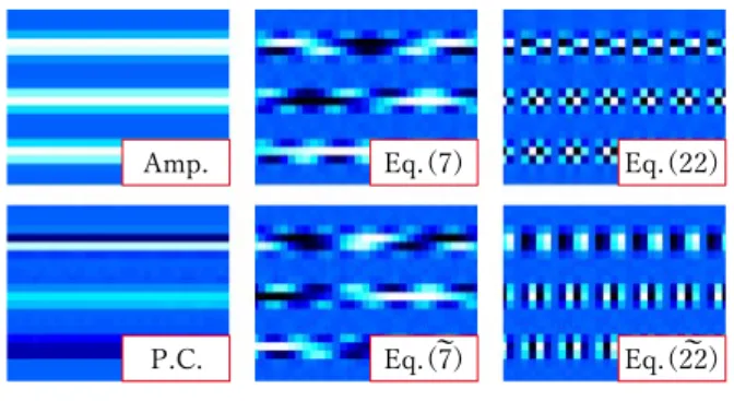
The effect of the phase correction is illustrated in Fig. 2, where the spectrograms consisting of three sinus-oids were calculated with different definitions, phase correction was calculated by Eq. (21), and the real parts
Phase conversion Phase inversion Process (complex) Convert to amplitude Process (real) Attach phase
(a) Ordinary amplitude-only processing scheme
(b) Proposed phase-aware processing scheme
Fig. 1 Comparison of the ordinary amplitude-based and the proposed phase-conversion-based frameworks (the input and output are complex spectrograms).
Eq.(7) Amp. P.C. Eq.(7) Eq.(22) Eq.(22) ~ ~
Fig. 2 Spectrograms of sum of 3 sinusoids. While amplitude is the same for all figures, their phase differs depending on the definition of DGT. For visual convenience, the real parts of the complex spectrogram are shown (except the top-left figure which illustrates the amplitude common for every other figures). Four representations on the right, calculated by Eqs. (7) and (22) (those with tildes were calculated with a zero-phased window), exhibit periodic patterns correspond-ing to the phase evolution. In contrast, the phase-corrected spectrogram on the bottom left is smooth along time.
10
Here, frequencies are considered in the unit of index.
11The reason for using cumulative sum of the relative instantaneous frequency ½m;n ¼Pnk¼1DtEq(7)½m;k is that DtEq(7) only represents the adjacent (local) relation, while the phase correction is based on the global relation½m;ngiven for allm;n.
are shown for visibility12. While amplitude is the same for all expressions, phase is different in accordance with the definition of DGT. By applying phase correction, phase evolution was canceled that can be seen from the figure at the bottom left. As sinusoids become smooth along time, phase correction has been applied to some applications enhancing/distinguishing sinusoidal components such as speech enhancement [1] and harmonic/percussive source separation [39].
4.4. Application: Complex Low-rankness
An interesting example of its property is that phase correction allows a complex spectrogram consisting of sinusoidal components to be rank [40]. While low-rank modeling of amplitude spectrograms including NMF (nonnegative matrix factorization) has been studied widely [41], there exists few research considering low-rankness of complex spectrograms [42]. This is because usual complex spectrograms are not low-rank owing to the phase evolution. Low-rankness of the phase-corrected spectro-gram might be another direction of low-rank modeling in acoustics as it is phase-aware.
5.
SIGNAL PROCESSING WITH
SPECTROGRAM CONSISTENCY
Spectrogram consistency is a popular property utilized in phase-aware signal processing. In this section, we briefly mention that phase correction in the previous section can be combined with spectrogram consistency.
5.1. Spectrogram Consistency in Nutshell
In most cases, DGT maps a time-domain signal into higher-dimensional representation, i.e., dimensionality of spectrogramNM is higher than that of the signalL. Such redundancy indicates that only theL-dimensional subspace within the NM dimensions directly corresponds to time domain. In other words, any component in the remaining (NML)-dimensional subspace does not affect the time-domain signal. Spectrograms are said to beconsistentwhen they do not contain any component in that (NML )-dimensional subspace. While DGT of any time-domain signal is a consistent spectrogram, it can easily be inconsistent after some time-frequency-domain signal processing. Since inconsistent spectrogram contains
inef-fective components, constraining signal processing meth-ods to output consistent spectrogram has been preferred by many researchers.
5.2. Phase Recovery Based on Consistency
Phase recovery is a branch of signal processing which aims to estimate better phase corresponding to the given spectrogram [43,44]. One popular application of spectro-gram consistency is phase recovery which, in such case, is formulated as a problem of finding a spectrogram, whose amplitude is close to the given one, within the consistent
L-dimensional subspace. To do so, DGT and its inverse are repeatedly applied in an iterative procedure so that the result is constrained to be consistent [45–47]. Such combination of forward and inverse DGT corresponds to the projection onto that subspace.
5.3. Phase Correction with Consistency
Time-frequency-domain signal processing can be con-strained to be consistent by applying it with the pair of forward and inverse DGT. However, nonlinear transform (such as taking absolute value) may complicate derivation and/or analysis of a signal-processing algorithm. As a simpler alternative, phase correction can be utilized to construct a phase-aware and consistent signal processing method [1,39,40].
By handling variables in time domain and processing complex spectrogram through DGT, the processed result can be searched within the consistent subspace. Phase correction allows to take advantage of the structure of spectrograms including time-directional smoothness and low-rankness which have been rarely considered in the context of spectrogram consistency. As phase correction is linear transform, it is easier than nonlinear transform in both theoretical and practical senses. Some recent finding suggests effectiveness of such phase-correction-based consistent signal processing [1,39,40], which should be worth investigating further.
6.
CONCLUSION
In this paper, several time-frequency representations, STFT and DGT with variation on their definitions, were summarized with emphasis on difference of phase and instantaneous frequency among them. Signal processing with phase conversion and its instantaneous-frequency-based version, or phase correction, was introduced instantaneous-frequency-based on the neighborhood relation of spectrogram. Their collaboration with spectrogram consistency was also mentioned shortly. Some research has suggested that time-frequency representation is a worthwhile topic for discussion also in deep-learning-based methods [47,48], and we hope that this paper (together with the supplemental MATLAB code) will be helpful for developing audio
12
Equation numbers indicate the definitions of DGTs. Those with tilde were calculated with the same but zero-phased window (index was rotated before FFT so that peak of the window becomes the first element, see the supplemental code). Making a window zero-phased removes the linear phase component caused by the mismatch of indexing between the signal and FFT (its frequency-domain counterpart is well-known: index is rotated so that the negative frequency follows after the Nyquist frequency).
signal processing with consideration of such representation in time-frequency domain.
REFERENCES
[1] K. Yatabe and Y. Oikawa, ‘‘Phase corrected total variation for audio signals,’’ Proc. IEEE Int. Conf. Acoust. Speech Signal Process. (ICASSP), pp. 656–660 (2018).
[2] H. G. Feichtinger and T. Strohmer, Eds.,Gabor Analysis and Algorithms: Theory and Applications (Birkha¨user, Boston, 1998).
[3] H. G. Feichtinger and T. Strohmer, Eds.,Advances in Gabor Analysis(Birkha¨user, Boston, 2003).
[4] O. Christensen, Frames and Bases: An Introductory Course (Birkha¨user, Boston, 2008).
[5] O. Christensen, An Introduction to Frames and Riesz Bases (Birkha¨user, Boston, 2016).
[6] P. G. Casazza and G. Kutyniok, Eds.,Finite Frames: Theory and Applications(Birkha¨user, Boston, 2013).
[7] K. Gro¨chenig, Foundations of Time-Frequency Analysis (Birkha¨user, Boston, 2001).
[8] T. Werther, Y. C. Eldar and N. N. Subbanna, ‘‘Dual Gabor frames: Theory and computational aspects,’’ IEEE Trans. Signal Process.,53, 4147–4158 (2005).
[9] S. Li, Y. Liu and T. Mi, ‘‘Sparse dual frames and dual Gabor functions of minimal time and frequency supports,’’J. Fourier Anal. Appl.,19, 48–76 (2013).
[10] N. Perraudin, N. Holighaus, P. L. Søndergaard and P. Balazs, ‘‘Designing Gabor windows using convex optimization,’’Appl. Math. Comput.,330, 266–287 (2018).
[11] T. Kusano, Y. Masuyama, K. Yatabe and Y. Oikawa, ‘‘Designing nearly tight window for improving time-frequency masking,’’arXiv 1811.08783(2018).
[12] Z. Cvetkovic, ‘‘On discrete short-time Fourier analysis,’’IEEE Trans. Signal Process.,48, 2628–2640 (2000).
[13] J. Kovacevic and A. Chebira, ‘‘Life beyond bases: The advent of frames (Part I),’’ IEEE Signal Process. Mag., 24, 86–104 (2007).
[14] J. Kovacevic and A. Chebira, ‘‘Life beyond bases: The advent of frames (Part II),’’IEEE Signal Process. Mag.,24, 115–125 (2007).
[15] I. Daubechies, A. Grossmann and Y. Meyer, ‘‘Painless non-orthogonal expansions,’’J. Math. Phys.,27, 1271–1283 (1986). [16] P. Balazs, D. Bayer, F. Jaillet and P. L. Søndergaard, ‘‘The pole behavior of the phase derivative of the short-time Fourier transform,’’ Appl. Comput. Harmon. Anal., 40, 610–621 (2016).
[17] N. Perraudin, N. Holighaus, P. Majdak and P. Balazs, ‘‘Inpainting of long audio segments with similarity graphs,’’ IEEE/ACM Trans. Audio Speech Lang. Process., 26, 1083– 1094 (2018).
[18] H. Kawahara, T. Irino and M. Morise, ‘‘An interference-free representation of instantaneous frequency of periodic signals and its application to F0 extraction,’’ Proc. IEEE Int. Conf. Acoust. Speech Signal Process. (ICASSP), pp. 5420–5423 (2011).
[19] S. Fenet, R. Badeau and G. Richard, ‘‘Reassigned time-frequency representations of discrete time signals and appli-cation to the constant-Q transform,’’Signal Process.,132, 170– 176 (2017).
[20] K. Kodera, C. D. Villedary and R. Gendrin, ‘‘A new method for the numerical analysis of non-stationary signals,’’ Phys. Earth Planet. Inter.,12, 142–150 (1976).
[21] D. J. Nelson, ‘‘Cross-spectral methods for processing speech,’’ J. Acoust. Soc. Am.,110, 2575–2592 (2001).
[22] S. A. Fulop and K. Fitz, ‘‘Algorithms for computing the time-corrected instantaneous frequency (reassigned) spectrogram, with applications,’’J. Acoust. Soc. Am.,119, 360–371 (2006). [23] F. Auger and P. Flandrin, ‘‘Improving the readability of time-frequency and time-scale representations by the reassignment method,’’IEEE Trans. Signal Process.,43, 1068–1089 (1995). [24] G. K. Nilsen, ‘‘Recursive time-frequency reassignment,’’IEEE
Trans. Signal Process.,57, 3283–3287 (2009).
[25] F. Auger, E. Chassande-Mottin and P. Flandrin, ‘‘On phase-magnitude relationships in the short-time Fourier transform,’’ IEEE Signal Process. Lett.,19, 267–270 (2012).
[26] F. Auger, P. Flandrin, Y. Lin, S. McLaughlin, S. Meignen, T. Oberlin and H. Wu, ‘‘Time-frequency reassignment and synchrosqueezing: An overview,’’ IEEE Signal Process. Mag.,30, 32–41 (2013).
[27] N. Holighaus, Z. Pru˚sˇa and P. L. Søndergaard, ‘‘Reassignment and synchrosqueezing for general time-frequency filter banks, subsampling and processing,’’ Signal Process., 125, 1–8 (2016).
[28] Z. Pru˚sˇa, P. Balazs and P. L. Søndergaard, ‘‘A noniterative method for reconstruction of phase from STFT magnitude,’’ IEEE/ACM Trans. Audio Speech Lang. Process., 25, 1154– 1164 (2017).
[29] D. Fourer and G. Peeters, ‘‘Fast and adaptive blind audio source separation using recursive Levenberg–Marquardt syn-chrosqueezing,’’Proc. IEEE Int. Conf. Acoust. Speech Signal Process. (ICASSP), pp. 766–770 (2018).
[30] A. Hiruma, K. Yatabe and Y. Oikawa, ‘‘Separating stereo audio mixture having no phase difference by convex clustering and disjointness map,’’ Proc. Int. Workshop Acoust. Signal Enhance. (IWAENC), pp. 266–270 (2018).
[31] A. Hiruma, K. Yatabe and Y. Oikawa, ‘‘Detection of clean time-frequency bins based on phase derivative of multichannel signals,’’Proc. Int. Congr. Acoust. (ICA), (2019).
[32] T. Oberlin, S. Meignen and V. Perrier, ‘‘Second-order synchrosqueezing transform or invertible reassignment? To-wards ideal time-frequency representations,’’ IEEE Trans. Signal Process.,63, 1335–1344 (2015).
[33] D. Pham and S. Meignen, ‘‘High-order synchrosqueezing transform for multicomponent signals analysis — With an application to gravitational-wave signal,’’IEEE Trans. Signal Process.,65, 3168–3178 (2017).
[34] R. Behera, S. Meignen and T. Oberlin, ‘‘Theoretical analysis of the second-order synchrosqueezing transform,’’Appl. Comput. Harmon. Anal.,45, 379–404 (2018).
[35] I. Daubechies and S. Maes, ‘‘A nonlinear squeezing of the continuous wavelet transform based on auditory nerve mod-els,’’Wavelets Med. Biol., pp. 527–546 (1996).
[36] I. Daubechies, J. Lu and H.-T. Wu, ‘‘Synchrosqueezed wavelet transforms: An empirical mode decomposition-like tool,’’ Appl. Comput. Harmon. Anal.,30, 243–261 (2011).
[37] T. Oberlin, S. Meignen and V. Perrier, ‘‘The Fourier-based synchrosqueezing transform,’’ Proc. IEEE Int. Conf. Acoust. Speech Signal Process. (ICASSP), pp. 315–319 (2014). [38] I. Bayram and M. E. Kamasak, ‘‘A simple prior for audio
signals,’’IEEE Trans. Audio Speech Lang. Process.,21, 1190– 1200 (2013).
[39] Y. Masuyama, K. Yatabe and Y. Oikawa, ‘‘Phase-aware harmonic/percussive source separation via convex optimiza-tion,’’ Proc. IEEE Int. Conf. Acoust. Speech Signal Process. (ICASSP), (2019).
[40] Y. Masuyama, K. Yatabe and Y. Oikawa, ‘‘Low-rankness of complex-valued spectrogram and its application to phase-aware audio processing,’’Proc. IEEE Int. Conf. Acoust. Speech Signal Process. (ICASSP), (2019).
[41] D. Kitamura, ‘‘Nonnegative matrix factorization based on complex generative model,’’Acoust. Sci. & Tech.,40, 155–161 (2019).
[42] K. Yatabe and D. Kitamura, ‘‘Determined blind source separation via proximal splitting algorithm,’’Proc. IEEE Int. Conf. Acoust. Speech Signal Process. (ICASSP), pp. 776–780 (2018).
[43] Y. Wakabayashi, ‘‘Speech enhancement using harmonic-structure-based phase reconstruction,’’ Acoust. Sci. & Tech., 40, 162–169 (2019).
[44] Y. Masuyama, K. Yatabe and Y. Oikawa, ‘‘Model-based phase recovery of spectrograms via optimization on Riemannian manifolds,’’ Proc. Int. Workshop Acoust. Signal Enhance. (IWAENC), pp. 126–130 (2018).
[45] Y. Masuyama, K. Yatabe and Y. Oikawa, ‘‘Griffin–Lim like phase recovery via alternating direction method of multi-pliers,’’IEEE Signal Process. Lett.,26, 184–188 (2019). [46] K. Yatabe, Y. Masuyama and Y. Oikawa, ‘‘Rectified linear
unit can assist Griffin–Lim phase recovery,’’Proc. Int. Work-shop Acoust. Signal Enhance. (IWAENC), pp. 555–559 (2018). [47] Y. Masuyama, K. Yatabe, Y. Koizumi, Y. Oikawa and N. Harada, ‘‘Deep Griffin–Lim iteration,’’ Proc. IEEE Int. Conf. Acoust. Speech Signal Process. (ICASSP), (2019).
[48] D. Takeuchi, K. Yatabe, Y. Koizumi, Y. Oikawa and N. Harada, ‘‘Data-driven design of perfect reconstruction filter-bank for DNN-based sound source enhancement,’’Proc. IEEE Int. Conf. Acoust. Speech Signal Process. (ICASSP), (2019).
Kohei Yatabe received his B.E., M.E., and Ph.D. degrees from Waseda University in 2012, 2014, and 2017, respectively. He is currently an assistant professor of the Department of Inter-media Art and Science, Waseda University. His research interests include optical and acoustical signal processing.
Yoshiki Masuyama received the B.E. degree from Waseda University in 2019. He is current-ly pursuing a M.E. degree in the Department of Intermedia Art and Science, Waseda University. His research interests include musical acoustics and acoustical signal processing using convex optimization technique.
Tsubasa Kusano received the B.E. and M.E. degrees from Waseda University in 2017 and 2018, respectively. He is currently pursuing a Ph.D. degree in the Department of Intermedia Art and Science, Waseda University. His re-search interests include signal processing based on functional data analysis and time-frequency analysis.
Yasuhiro Oikawa received his B.E., M.E., and Ph.D. degrees in Electrical Engineering from Waseda University in 1995, 1997, and 2001, respectively. He is a professor of the Department of Intermedia Art and Science, Waseda University. His main research interests are communication acoustics and digital signal processing of acoustic signals. He is a member of ASJ, ASA, IEICE, IEEE, IPSJ, VRSJ, and AIJ.