A Case-Study in Programming Coinductive
Proofs: Howe’s Method
Alberto Momigliano1, Brigitte Pientka2 and David Thibodeau2 1 Dipartimento di Informatica, Universit`a degli Studi di Milano, Italy 2
School of Computer Science, McGill University, Montreal, Canada Received Received: date / Accepted: date
Bisimulation proofs play a central role in programming languages in establishing rich properties such as contextual equivalence. They are also challenging to mechanize, since they require a combination of inductive and coinductive reasoning on open terms. In this paper we describe mechanizing the property that similarity in the call-by-name lambda calculus is a pre-congruence using Howe’s method in theBelugaformal reasoning system. The development relies on three key ingredients: 1) we give a higher-order abstract syntax (HOAS) encoding of lambda-terms together with their operational semantics as intrinsically typed terms, thereby avoiding not only the need to deal with binders, renaming and substitutions, but keeping all typing invariants implicit; 2) we take advantage of Beluga’s support for representing open terms using built-in contexts and simultaneous substitutions: this allows us to directly state central definitions such as open simulation without resorting to the usual inductive closure operation and to encode very elegantly notoriously painful proofs such as the substitutivity of the Howe relation; 3) we exploit the possibility of reasoning by coinduction inBeluga’s reasoning logic. The end result is succinct and elegant, thanks to the high-level abstractions and primitives Belugaprovides. We believe that this mechanization is a significant example that illustratesBeluga’s strength at mechanizing challenging (co)inductive proofs using higher-order abstract syntax encodings.
1. Introduction
Logical frameworks such as LF (Harper et al., 1993) andλProlog (Miller and Nadathur, 2012) provide a meta-language for representing formal systems given via axioms and inference rules, factoring out common and recurring issues such as modelling variable bindings. They exploit the idea, dating back to Church, to use a lambda calculus as the meta-language to uniformly encode variable binding in our formal system. (HOAS) or (in a slightly weaker setting) “lambda”-tree syntax (Miller and Palamidessi, 1999). In particular, we can encode uniformly variable binding operators by mapping them to the lambda binder of the meta-language. As a consequence variables in the object lan-guage (OL) are represented by variables in the meta-lanlan-guage (ML) and inherit thereby α-renaming and substitution from it. Moreover, this encoding technique scales to rep-resenting formal systems that use hypothetical and parametric reasoning by providing
generic support for managing hypotheses and the corresponding substitution lemmas. As users do not need to build up all this basic mathematical infrastructure, it is easier to prototype proof environments and mechanize formal systems. It can also have substantial benefits for proof checking and proof search.
While representing formal systems is a first step, the interesting question is how we can reason about HOAS representations inductively. Meta-languages such as LF orλ-Prolog that are used for representing OL are weak calculi and do not include case analysis, recursion or inductive definitions. This is in fact essential to achieve an adequate repre-sentation of the OL where each OL term uniquely corresponds to a given reprerepre-sentation in the meta-language. So, how can we still reason about such representations?
One solution to this conundrum is the so-called “two-level” approach, as advocated by McDowell and Miller (1997), where we distinguish between a specification language and a reasoning logic above it, which supports at least some form of induction. The cited paper presented FOLDN, which is basically a first order logic with definitions (fixed points) and natural number induction. Object logics are encoded in a specification language, which may vary and often is based on (possibly sub-structural) fragments of hereditary Harrop formulas. The method was tested on classical benchmarks such as subject reduction for PCF and its imperative variants.
Notably, one of Dale Miller’s motivating examples has been the (meta)theory of process calculi, in particular theπ-calculus. This brought to the forefront the issue of representing and reasoning aboutinfinite behaviour. In fact, McDowell et al. (1996) were concerned with the representation of transition systems and their bisimulation: in agreement with Milner’s original presentation inA Calculus of Communicating Systems, bisimilarity was capturedinductivelyby computing the greatest fixed point starting from the universal re-lation and closing downwards by intersection. This is doable, but notoriously awkward to work with and in fact Milner swiftly adopted the notion ofcoinduction in his subsequent Communication and Concurrency.
In the late 1990, coinduction was available in general proof assistants such as Is-abelle/HOL and Coq, the first by encoding the standard Tarski’s fixed point theorem in higher order logic, the latter by guarded induction; several reasonably large case studies were carried out, not without some difficulties (Ambler and Crole, 1999; Honsell et al., 2001; Hirschkoff, 1997). These case studies further demonstrated the challenges in mod-elling variable bindings and building up such an infrastructure, as lambda-tree syntax is fundamentally incompatible with the foundations of these proof systems. It turns out instead that it is quite natural to step from FOLDN to support (co)inductive reason-ing; Momigliano and Tiu (2003) adopted the view of definitions as least and greatest fixed points adding rules for fixed point induction. This was later shown to be consistent (Tiu and Momigliano, 2012). With the orthogonal ingredient of∇-quantifier to abstract over variable names (Miller and Tiu, 2005), this line of research culminated in theAbellaproof assistant (Baelde et al., 2014), which until recently was the only proof assistant support-ing natively both HOAS and coinduction, as exemplified in some non-insignificant case studies (Tiu and Miller, 2010; Momigliano, 2012).
Pfen-ning advocated using it as a meta-logical framework by representing inductive proofs as relations. To ensure that a relation describes a valid inductive proof, external checks guarantee that the implemented relation constitutes a total function, i.e. covers all cases and all appeals to the induction hypothesis are well-founded. This lead to the proof environment Twelf (Pfenning and Sch¨urmann, 1999), which has been used widely, see for a major case study (Lee et al., 2007). However,Twelf did not seem to lend itself to coinductive reasoning.
To address these and other shortcomings, Pientka (2008) designed a reasoning logic on top of LF that allows us to directly analyze and manipulate LF objects.Beluga(Pientka and Dunfield, 2010) implements this idea. To model derivation trees that depend on as-sumptions, LF objects are paired with their surrounding context (Nanevski et al., 2008; Pientka, 2008; Pientka and Dunfield, 2008). Inductive proofs are then implemented as recursive functions that directly pattern match on contextual LF objects. Beluga pro-vides a proof language that makes explicit context reasoning via built-in contexts and simultaneous substitutions together with their equational theory. Moreover, it supports inductive and stratified definitions in addition to higher-order functions (Cave and Pien-tka, 2012; Pientka and Cave, 2015; Jacob-Rao et al., 2018), thereby going substantially beyond the expressive power of Twelf.
One might say that the proof and the type-theoretic approaches are converging to-wards a core reasoning logic that supports least and greatest fixed points and equality within first-order logic. This might be more obvious in the inductive case where we are more familiar with the computational interpretation of proofs: we readily interpret pattern matching in a program as case analysis in a proof and accept that recursive calls on structurally smaller objects correspond to well-founded appeals to the induc-tion hypothesis. Coinductive reasoning in type theory is less well understood. In fact, guarded co-recursion in Coq, for example, does not preserve types (Oury, 2008). To overcome these and other difficulties, Pientka and collaborators (Abel et al., 2013; Abel and Pientka, 2016; Thibodeau et al., 2016) proposed in prior work a novel computational interpretation of coinductive proofs. While finite (inductive) data is defined using con-structors and analyzed viapattern matching, we define infinite (coinductive) data by the observations that we can make about it. We can reason about such observations using copattern matching. A function about finite data represents an inductive proof, if we cover all cases and all recursive calls are on structurally smaller objects. This guarantees that the function istotal, that is, defined on all inputs and terminating. Dually, a total function about infinite data corresponds to a coinductive proof, if we cover all possible observations on the output and all recursive calls are guarded by an observation. This guarantees that the function is defined on all possible outputs and remains productive, as we only proceed to evaluate the co-recursive function when we apply it to an observation. As a contribution to a better understanding of the relationship between the logical and computational interpretation of coinductive proofs, the present paper reappraises the proof that similarity in the call-by-name lambda calculus with lists is a pre-congruence using Howe’s method (Howe, 1996). This is a challenging proof since it requires a com-bination of inductive and coinductive reasoning on open terms. We mechanize this proof inBeluga, relying on three key ingredients:
1. we give a HOAS encoding of lambda-terms together with their operational semantics asintrinsically typed terms, thereby avoiding not only the need to deal with binders, renaming and substitutions, but keeping all typing invariants implicit;
2. we take advantage of Beluga’s support for representing open terms using built-in contexts and simultaneous substitutions: this allows us to directly state a notion such as open simulation without resorting to the usual inductive closure operation and to encode neatly notoriously painful proofs such as the substitutivity of the Howe relation;
3. we exploit the possibility of reasoning by coinduction inBeluga’s reasoning logic. The end result is, in our opinion, succinct and elegant, thanks to the high-level ab-stractions and primitivesBelugaprovides.
The paper starts in Section 2 with a summary description of Howe’s method and discusses the challenges that it poses to its mechanization. The latter is detailed in Sec-tion 3, together with a proof of adequacy of our encoding of similarity (SecSec-tion 3.4) and a example derivation of two terms being similar (Section 3.6). We review related work in Section 4 and conclude in Section 5. Appendix A contains a brief overview of the relevant part of Beluga’s syntax. The entire formal development can be retrieved fromhttps:// github.com/Beluga-lang/Beluga/tree/master/examples/codatatypes/howes-method.
2. A summary of Howe’s method
First let us fix our programming languages as the simply-typedλ-calculus with recursion over (lazy) lists, which we callPCFLfollowing Pitts (1997). Its types consist of the unit type (written as>), function types, and lists (written aslist(τ)).
Types τ ::= > |τ→τ |list(τ)
Terms m, n, p, q ::= x|lamx. p|m1 m2|fixx. m| hi
|nil|consmh mt|lcasemof {nil⇒n|conshd tl⇒p}
Values v ::= hi |lamx. p|nil|consmh mt
The typing rules for PCFL and the big step lazy operational semantics denoted by m⇓v are standard and we omit them here. In particular, lists are only evaluated lazily, as the definition of values shows. The interested reader can skip ahead to their encoding in LF in the Section 3.1 or consult Pitts (1997).
2.1. Proving bisimilarity a congruence using Howe’s method
Suppose we want to say when two programs (two closed terms) have the same behavior. A well known characterization is Morris-stylecontextual equivalence: occurrences of the first expression in any program can be replaced by the second without affecting the observable results of executing the program
about it, mainly due to the quantification on every possible context.† Many techniques have been proposed through the years, ranging from domain theory (Abramsky, 1991), game semantics (Ghica and McCusker, 2000) to logical relations (Ahmed, 2006). The idea of bisimilarity has usefully been adapted from concurrency theory to provide yet another characterization of contextual equivalence. Bisimilarity is, similarly to contextual equivalence, parametrized by the notion ofobservable we select: roughly, m and n are bisimilar if wheneverm evaluates to an observable so does n, and all the subprograms of those are also bisimilar. In the case ofapplicative bisimilarity, evaluation at function type is pushed until values are reached.
To simplify the presentation, we will concentrate on the notion ofsimilarity, from which bisimilarity can be obtained by symmetry, that is taking the conjunction of similarity and its inverse; this is possible thanks to determinism of evaluation.
Definition 1 (Applicative simulation). Anapplicative simulationis a family of typed relationsRτ on closed terms satisfying the following conditions:
—ifmR> nthenm⇓ hientailsn⇓ hi. —ifmRlist(τ)nthenm⇓nilentailsn⇓nil.
—if m Rlist(τ) n then m ⇓ cons mh mt entails that there are terms m0h and m0t such that n⇓consm0hm0tfor whichmhRτ m0handmt Rlist(τ) m0t.
—ifmRτ→τ0 nthenm⇓lamx. m0 entails that there is a termn0such thatn⇓lamy. n0
for whichm0[r/x]Rτ0 n0[r/y] for every termrof typeτ.
We can make sense of the non-well-founded nature of the last two conditions by noting that there are non-empty simulations, e.g. the identity relation and that the union of two applicative simulations is still a simulation. Hence there exists thelargestone, which we call applicativesimilarity. This relation can also be characterized using the Knaster-Tarski fixed point theorem, as the greatest fixed point of an appropriate endofunction Φ on families of typed relations. For a detailed explanation we refer again to Pitts (1997), and we just mention that the definition of the function follows the simulation relation, and has, for example atτ →τ0, mΦ(Rτ→τ0)njust in case whenever m⇓lamx. m0 for
anym0, there exists a termn0 such thatn⇓lamy. n0 and for everyrof typeτ,m0[r/x] is Rτ0-related ton0[r/y]; hence, similarity is the set coinductively defined by Φ, a relation
we write as m 4τ n. This yields a co-induction principle that we describe first in its generality and below we show it instantiated to applicative similarity.
∃S s.t.a∈S S⊆Φ(S) CI a∈gfp(Φ) ∃Sτ s.t.m Sτ n Sτ is an applicative simulation CI− m4τ n
It is not difficult to show that similarity is a pre-order and we detail the proof of
†This notion can and has been simplified, starting from Milner’s context lemma (Milner, 1977) and go-ing through the CIU theorem (Mason and Talcott, 1991). Some mechanizitions are also available (Ford and Mason, 2003; McLaughlin et al., 2018), as we discuss further in Section 4.
reflexivity using ruleCI− to highlight the similarities with the type-theoretic definition based instead on the notion of observation, on which our mechanization relies.
Theorem 1 (Reflexivity of applicative similarity). ∀m τ, m4τ m.
Proof. To show the result we need to provide an appropriate simulationS and check the simulation conditions. Just chooseSτ to be the family{(m, m)| · `m:τ}where we use the judgmentm:τ to say that termmhas typeσ.
We then consider each case in the applicative simulation definition. —ifmS> m, thenm⇓ hientailsm⇓ hi: immediate;
—ifmSlist(τ)m, thenm⇓nilentailsm⇓nil: immediate; —assume m Slist(τ) m and m ⇓ cons mh mt; pick m0h, m
0
t to be mh, mt and by the definition of the simulation, it holds thatmh Sτ mh andmtSlist(τ) mt;
—assumemSτ→τ0mandm⇓lamx. m0; again by pickingm0forn0and by the definition
of the simulation it is obvious that for every r:τ, [r/x]m0 Sτ0 [r/x]m0.
In many cases, we do not have to look much further beyond the statement of the theorem to come up with an appropriate simulation, i.e. we can read off the definition of simulation from it — and this is indeed the case for all the coinductive proofs in the following development. However, to show the equivalence of specific programs we may have to come up with a complex bisimulation, possibly defined inductively and/or “up to”. This phenomenon is well-known in inductive theorem proving, where sometimes the induction hypothesis coincides with the statement of the theorem, but in other cases it needs to be generalized in an appropriate lemma. The fixed point rules conflate those two aspects, generalization and lemma application, in one go. With an abuse of language, we will say that we prove a statement by coinduction and say that we appeal to the use of the “coinductive hypothesis” when the simulation corresponds to the statement of the theorem.
When dealing with program equivalence,equational (in addition to coinductive) rea-soning would be helpful and this is why it is crucial to establish bisimilarity to be a congruence, i.e. a relation respecting the way terms are constructed. Since in this pa-per we restrict ourselves to similarity, we targetpre-congruence. Given the presence of variable-binding operators, we need to consider relations overopenterms, that is families of relations over terms indexed by a typing context Γ in addition to a typeτ, which we write as Γ`mRτ n.
Definition 2 (Compatible relation). A relation Γ`mRτ niscompatible when: (C0)Γ` hi R> hi;
(C1)Γ, x:τ`xRτ x;
(C2)Γ, x:τ`mRτ0 nentails Γ`(lamx. m)Rτ→τ0 (lamx. n);
(C3)Γ`m1 Rτ→τ0 n1 and Γ`m2 Rτ n2entail Γ`(m1 m2)Rτ0 (n1 n2);
(C4)Γ, x:τ`mRτ nentails Γ`(fixx. m)Rτ (fixx. n);
(C5a)Γ`mhRτ nhand Γ`mtRlist(τ)ntentail Γ`(consmh mt)Rlist(τ)(consnh nt); (C5b)Γ`nilRlist(τ)nil;
(C6)Γ ` m1 Rlist(τ) m2, Γ ` n1 Rτ0 n2 and Γ, h:τ, t:list(τ) ` p1 Rτ0 p2 entail Γ `
(lcasem1 of {nil⇒n1|conshd tl⇒p1})Rτ0(lcasem2of {nil⇒n2|conshd tl⇒p2}).
Definition 3 (Pre-congruence). Apre-congruenceis a compatible transitive relation. By the very definition of simulation at arrow type it is clear that a key property for our development is for a relation to be preserved by pairwise substitution:
Γ, y:τ `m1 Rτ0 m2 and Γ`n1Rτ n2 entails Γ`[n1/y]m1 Rτ0 [n2/y]m2.
We generalize this property here using simultaneous substitutions, streamlining our formal development, see Section 3.7. Fig. 1 gives rules for well-typed simultaneous sub-stitutions Ψ`σ: Γ, where σreplaces variables in Γ with terms typable in Ψ; then, we state when two such substitutions areR-related:
Well-Typed Simultaneous Substitutions: Ψ`σ: Γ
Ψ` ·:·
Ψ`σ: Γ Ψ`m:τ
Ψ`σ, m/x: Γ, x:τ
Related Simultaneous Substitutions: Ψ`σ1 RΓσ2
Ψ` · R··
Ψ`σ1 RΓσ2 Ψ`mRτ n
Ψ`(σ1, m/x)RΓ,x:τ (σ2, n/x) Fig. 1. (Related) simultaneous substitutions
Definition 4 (Substitutive relation). A relation issubstitutive(Sub)iff Γ`m1Rτm2 and Ψ`σ1RΓ σ2entails Ψ`[σ1]m1 Rτ [σ2]m2.
Some other properties are admissible:
Lemma 2 (Elementary admissible properties).
(Ref ) If a relation is compatible, then it is reflexive; further, if Γ ` m Rτ m, then Ψ`σRΓ σ.
(Cus) IfRτ is substitutive and reflexive, then it is alsoclosed under substitution: Γ`m1 Rτ m2 and Ψ`σ: Γ entails Ψ`[σ]m1 Rτ [σ]m2.
Weakening (Wkn), that is Γ`mRτ nand Γ⊆Γ0 entailing Γ0 `mRτ n, follows from Cus takingσto be the identity substitution for Γ.
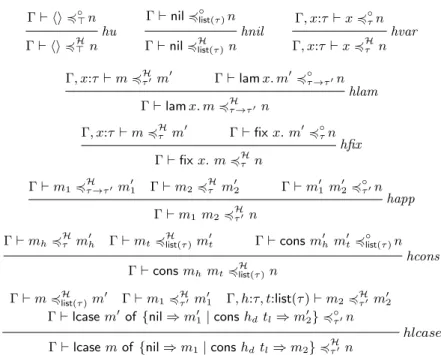
The definition of similarity applies only to closed terms. It is therefore customary to extend similarity toopen terms via substitution. We do this using grounding substitu-tions:
Γ` hi4◦>n hu Γ` hi4H>n Γ`nil4◦list(τ)n hnil Γ`nil4Hlist(τ)n Γ, x:τ `x4◦τn hvar Γ, x:τ`x4Hτ n Γ, x:τ `m4Hτ0 m0 Γ`lamx. m04◦τ→τ0n hlam Γ`lamx. m4Hτ→τ0 n Γ, x:τ `m4Hτ m 0 Γ`fixx. m04◦τn hfix Γ`fixx. m4Hτ n Γ`m14 H τ→τ0 m01 Γ`m24 H τ m 0 2 Γ`m 0 1 m 0 24 ◦ τ0n happ Γ`m1 m24Hτ0 n Γ`mh4 H τ m 0 h Γ`mt4 H list(τ)m 0 t Γ`consm 0 hm 0 t4 ◦ list(τ)n hcons Γ`consmhmt4 H list(τ)n Γ`m4Hlist(τ)m 0 Γ`m14Hτ0 m01 Γ, h:τ, t:list(τ)`m24Hτ0 m02 Γ`lcasem0 of {nil⇒m01|conshdtl⇒m02}4◦τ0n
hlcase
Γ`lcasemof{nil⇒m1|cons hdtl⇒m2}4Hτ0 n
Fig. 2. Definition of the Howe relation
Now, it is immediate that open similarity is a pre-order and hence (C1) and transitivity hold. Further, (C2) also holds, since similarity satisfies
lamx. m4τ→τ0 lamx. niff for allp:τ, [p/x]m4τ0 [p/x]n
However, a direct attempt to prove pre-congruence of open similarity breaks down when dealing with (C3) and (C6). Moreover, while it follows simply by construction that open similarity is closed under substitution, it is not obvious that it is substitutive.
Howe’s idea (Howe, 1996) was to introduce acandidaterelation4Hτ (see Fig. 2), which contains (open) similarity and can be shown to be almost a substitutive pre-congruence, and then to prove that it does coincide with similarity.
The informal proof consists of several lemmata:
(1) Semi-transitivity: the composition of the Howe relation with open similarity is con-tained in the former. The proof goes by case analysis on the derivation of the Howe relation using transitivity of open similarity.
(2) The Howe relation is reflexive. Induction on typing, using reflexivity of open similarity. (3) Compatibility: (C0)—(C6) hold, an easy consequence of (2).
(4) Open similarity is contained in Howe, which follows immediately from (1) and (2). (5) The Howe relation is substitutive, see Lemma 6.
(6) The Howe relation “mimics” the simulation conditions: (6.1) If hi4H
> n, thenn⇓ hi. (6.2) If nil4Hlist(τ)n, thenn⇓nil.
(6.3) If lamx. m4Hτ→τ0 n, then n⇓ lamx. m0 and for everyq:τ we have [q/x]m 4Hτ0
(6.4) If consmh mt4Hlist(τ)n, thenn⇓consph pt, withmh4Hτ ph andmt4Hlist(τ)pt. By inversion on the Howe relation and definition of similarity, using semi-transitivity and, in the lambda-case, substitutivity of the Howe relation.
(7) Downward closure: ifp4Hτ q andp⇓v, thenv4Hτ q. Induction on evaluation, and inversion on the Howe relation and similarity, with an additional case analysis onv. (8)p4Hτ q entails p4τ q. By coinduction, using the coinductive hypothesis, point (6)
and (7).
Once all of these properties have been proved, we are ready for the main result, stating that the Howe relation coincides with applicative similarity, and hence the pre-congruence of the latter follows as a corollary:
Theorem 3. Γ`p4Hτ qiff Γ`p4◦τq
Proof. Right to left is point (4) above. Conversely, proceed by induction on Γ using (8) for the base case and closure under substitution for the step.
Corollary 1. Open similarity is a pre-congruence.
2.2. On the role of substitutions in Howe’s method
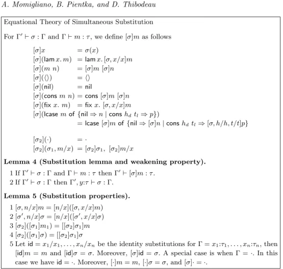
Substitutions play a central role in the overall proof that similarity is a pre-congruence. In the informal proof, we silently exploit equational laws about substitution; however, they can cause significant trouble during mechanization. We summarize the definition of substitution for our term language together with its equational theory in Fig. 3. To illustrate how we rely on these substitution properties in proofs, we show here in more detail the proof of substitutivity and pay particular attention to the properties in Fig. 3. Recall that the definition of Ψ`σ14HΓ σ2 is just an instance of the definition of related simultaneous substitutions.
Lemma 6 (Substitutivity of the Howe relation). Suppose we have Γ`m14Hτ m2 and Ψ`σ14HΓ σ2; then Ψ`[σ1]m14Hτ [σ2]m2.
Proof. By induction on the derivations of Γ`m14Hτ m2.
Case Γ`m4Hτ→τ0 m0 Γ`n4Hτ n0 Γ`m0 n04◦τ0r happ Γ`m n4Hτ0 r Ψ`[σ1]m4Hτ→τ0 [σ2]m0 by IH on first subderivation Ψ`[σ1]n4Hτ [σ2]n0 by IH on second subderivation Ψ`[σ2](m0 n0)4◦τ0[σ2]r by cus on third subderivation
[σ2](m0 n0) = [σ2]m0 [σ2]n0 by def. of substitution (see Fig. 3)
Ψ`[σ1]m [σ1]n4Hτ0 [σ2]r by rulehapp
Equational Theory of Simultaneous Substitution For Γ0`σ: Γ and Γ`m:τ, we define [σ]mas follows
[σ]x =σ(x) [σ](lamx. m) =lamx.[σ, x/x]m [σ](m n) = [σ]m[σ]n [σ](hi) =hi [σ](nil) =nil [σ](consm n) =cons[σ]m[σ]n [σ](fixx. m) =fixx.[σ, x/x]m
[σ](lcasemof {nil⇒n|conshdtl⇒p})
=lcase[σ]mof{nil⇒[σ]n|conshd tl⇒[σ, h/h, t/t]p}
[σ2](·) =·
[σ2](σ1, m/x) = [σ2]σ1, [σ2]m/x
Lemma 4 (Substitution lemma and weakening property).
1 If Γ0`σ: Γ and Γ`m:τ then Γ0`[σ]m:τ. 2 If Γ0`σ: Γ then Γ0, y:τ`σ: Γ.
Lemma 5 (Substitution properties).
1 [σ, n/x]m= [n/x]([σ, x/x]m) 2 [σ0, n/x]σ= [n/x]([σ0, x/x]σ) 3 [σ2]([σ1]m1) = [[σ2]σ1]m 4 [σ2]([σ1]σ) = [[σ2]σ1]σ
5 Letid=x1/x1, . . . , xn/xnbe the identity substitutions for Γ =x1:τ1, . . . , xn:τn, then
[id]m=m and [id]σ=σ. Moreover, [σ]id =σ. A special case is when Γ =·. In this case we haveid=·. Moreover, [·]m=m, [·]σ=σ, and [σ]·=·.
Fig. 3. Properties of simultaneous substitutions
Case Γ, x:τ`m4Hτ0 m0 Γ`lamx. m0 4◦τ→τ0r hlam Γ`lamx. m4Hτ→τ0 r Ψ`σ14HΓ σ2 by assumption Ψ, x:τ`σ14HΓ σ2 by weakening (Lemma 4.2)
[σ]x4τ[σ]xfor anyσwhere· `σ: Ψ, x:τ by reflexivity of similarity (Theorem 1
Ψ, x:τ`x4◦τx by def. of open similarity
Ψ, x:τ`x4Hτ x by rulehvar
Ψ, x:τ`σ1, x/x4HΓ,x:τσ2, x/x by def. of Howe related substitutions Ψ, x:τ`[σ1, x/x]m4Hτ0 [σ2, x/x]m0 by IH on first subderivation Ψ`[σ2](lamx. m0)4◦τ→τ0[σ2]r by cus on second subderivation
[σ2](lamx. m0) =lamx.[σ2, x/x]m0 by def. of substitution (see Fig. 3) Ψ`(lamx.[σ1, x/x]m)4Hτ→τ0 [σ2]r by rulehlam
Ψ`[σ1](lamx. m)4Hτ→τ0 [σ2]r by above line
The other cases are analogous.
3. Mechanizing Howe’s method inBeluga
We discuss in this Section the proof that similarity in PCFLis a pre-congruence using Howe’s method inBeluga.
Belugais a programming environment that supports both specifying formal systems and reasoning about them. To specify formal systems such as PCFLwe use the logical framework LF. This allows us to take advantage of higher-order abstract syntax. A key challenge when reasoning about LF objects is that we must consider potentially open objects. InBeluga, this need is met by viewing all LF objects together with the contexts in which they are meaningful (Nanevski et al., 2008) as contextual LF objects and by abstracting not only over LF objects but also over contexts. We then view contextual objects and contexts as a particular index domain about which we can reason using a first-order logic with (co)induction principles on our index domain and built-in equality on index objects. Under the Curry-Howard isomorphism this logic corresponds to a func-tional language with indexed (co)inductive types that supports (co)pattern matching. Meta-theoretic proofs about formal systems are implemented as (co)recursive functions in Beluga. We summarize in Appendix A the source level syntax of Beluga, where we concentrate on the parts that are relevant for our development. It is by no means a com-plete description, but it may serve as a useful high-level introduction to understanding Belugaprograms. For a more formal introduction to the theoretical foundations, we refer the reader to (Cave and Pientka, 2012; Thibodeau et al., 2016).
3.1. Encoding syntax in LF
We adopt the usual HOAS encoding for binding operators in the object language, and make essential use of LF’s dependent types (see Fig. 4). In particular the type family
term encodes intrinsically-typed terms. This will make our overall mechanization more compact, as all terms are well-typed by construction which is enforced byBeluga’s type checker.
Variables such as T and S that are used in declaring the type of the LF constants are abstracted over at the front of the type of the constructor and we rely on type reconstruction to infer their types (Pientka, 2013). These variables are treated as implicit and we subsequently omit passing them when formingterm objects.
3.2. Encoding the operational semantics with indexed inductive types
To illustrate how we can use inductive types inBeluga, we encode thevalueandevaluation judgment as computation-level type families indexed by closed well-typed terms. This is demonstrably equivalent to encoding the same judgments at the LF level.
How do we enforce that a LF object is closed? This is accomplished by a contextual
LF tp : type = | top : tp
| arr : tp → tp → tp
| list: tp → tp;
LF term : tp → type =
| app : term (arr S T) → term S → term T
| lam : (term S → term T) → term (arr S T)
| fix : (term T → term T) → term T
| unit : term top
| nil : term (list T)
| cons : term T → term (list T) → term (list T)
| lcase: term (list S) → term T → (term S → term (list S) → term T)
→ term T;
Fig. 4. LF definition of intrinsically typed terms
inductive Value : [term T] → ctype =
| Val_lam : Value [lam λx.N]
| Val_unit : Value [unit]
| Val_nil : Value [nil]
| Val_cons : Value [cons M1 M2];
inductive Eval : [term T] → [term T] → ctype =
| Ev_app : Eval [M1] [lam λx.N] → Eval [N[M2]] [V]
→ Eval [app M1 M2] [V]
| Ev_val : Value [V]
→ Eval [V] [V]
| Ev_fix : Eval [M[fix λx.M]] [V]
→ Eval [fix λx.M] [V]
| Ev_case_nil : Eval [M] [nil] → Eval [M1] [V]
→ Eval [lcase M M1 (λh.λt.M2)] [V]
| Ev_case_cons: Eval [M] [cons H L] → Eval [M2[H, L]] [V]
→ Eval [lcase M M1 (λh.λt.M2)] [V];
Fig. 5. Inductive definition of values and evaluation
empty; to improve readability we simply write[term T]. Note that we can embed
contex-tual types intoBelugatypes, but not vice-versa. There is a strict separation between LF definitions that form our index objects andBelugatypes that talk about LF definitions. The inductive type family Value defines a subset of closed well-typed expressions, namely those that are the observables of our OL. Similarly, the inductive type family
Eval relates two closed expressions of the same type, where the first big-step evaluates to the second (see Fig. 5).
Belugahas a sophisticated notion of built-in simultaneous substitution. Consider the
ruleEv_app, where to build the evaluation derivation forEval [app M1 M2] [V]we have to
supply an evaluation derivation forEval [M1] [lam λx.N]andEval [N[M2]] [V]whereN
stands for a term of typeSthat may refer tox:term T. The substitution that in standard LF would be represented as meta-level application N M2, here consists of the singleton simultaneous substitutionN[M2]that keeps its domain, namelyx, implicit. In general, all capitalized variables denote LF objects that may depend on LF declarations. Given an LF termNthat depends on a contextγ, we can useNin a contextψby associatingNwith a simultaneous substitutionσwith domainψand co-domainγ, with type[ψ ` γ]. This closure is written in post-fix notation asN[σ]. If σis the identity substitution, we may
drop the closure. We make use of two kinds ofweakening substitutions: 1) The weakening substitution, written as [], moves a closed object from the empty context to a context γ. For example, the type Tis closed in [term T]. To use the closed type Tin a context γ, we need to associate it with the weakening substitution []. Hence, [γ ` term T[]]
describes atermobject of typeTin a contextγand enforces that the typeTis closed. The weakening substitution, written as[...], moves an objectMthat is defined in a contextγ
to an extension ofγ, for exampleγ, x:term T[]. Finally, we note that[lam λx.N]can be
expanded to[lam λx.N[x]]where the substitution that mapsxto itself is simply written as[x].
Inductive types inBelugacorrespond to least fixed points over an index domain type-theoretically defined using labelled sums and Σ-type (Cave and Pientka, 2012; Thibodeau et al., 2016). Such inductive types must in general satisfy the positivity condition. The surface definition of Valueis translated in the following notation where sums are repre-sented as list of labels together with their computation-level types wrapped with< >.
µValue.λT, M.
<Val lam: ΣS1, S2:[tp].T = (arrS1 S2)×ΣN:[x:termS1`termS2[]].M =lamλx.N,
Val unit:T =top×M =unit,
Val nil : ΣS:[tp].T=listS×M =nil
Val cons: ΣS:[tp].T=listS×ΣM1:[termS].ΣM2:[term(listS)]. M=consM1M2>
We use equality constraints to express the refinement of the indices T and M in the above encoding. In general, our index domain is contextual LF (Cave and Pientka, 2012, 2013), which has canonical forms. Hence, checking whether two contextual LF objects are equal simply boils down to comparing their canonical form.
We viewValueas a least fixed point definition, although in this case there is no recursive reference toValue. The latter happens in the fragment of the inductive type forEval:
µEval.λT, M, W.
<Ev app: ΣS:[tp], M1:[term(arrS T)], M2:[termS], N:[x:termT `termS[]]. M = (appM1 M2)×Eval[M1] [lamλx.N]×Eval[N[M2]] [W]
E fix: ΣN:[x:termT `termT[]]. M=fixλx.N×Eval[N[fixλx.N]] [W]
3.3. Encoding similarity using indexed coinductive types
InBeluga, we also can state coinductive type families and in particular similarity as a coinductive definition that relates closed well-typed terms.
coinductive Sim : {T:[tp]} [term T] → [term T] → ctype =
| (Sim_unit : Sim [top] [M] [N])
:: Eval [M] [unit] → Eval [N] [unit]
| (Sim_nil : Sim [list T] [M] [N])
:: Eval [M] [nil] → Eval [N] [nil]
| (Sim_cons : Sim [list T] [M] [N])
:: Eval [M] [cons H L] → Ex_sim_cons [H] [L] [N]
| (Sim_lam : Sim [arr S T] [M] [N])
:: Eval [M] [lam λx.M’] → Ex_sim_lam [x:term S ` M’] [N]
and inductive Ex_sim_cons : [term T] → [term (list T)] → [term (list T)]
→ ctype =
| ESim_cons: Eval [N] [cons H’ L’]
→ Sim [T] [H] [H’] → Sim [list T] [L] [L’]
→ Ex_sim_cons [H] [L] [N]
and inductive Ex_sim_lam : [x:term S ` term T[]] → [term (arr S T)]
→ ctype =
| ESim_lam: Eval [N] [lam λx.N’]
→ ({R:[term S]} Sim [T] [ M’[R] ] [ N’[R] ])
→ Ex_sim_lam [x:term S ` M’] [N]
Fig. 6. Coinductive definition of applicative similarity
While inductive types are defined by constructors, we characterize coinductive types by theobservationswe can make (Abel et al., 2013; Thibodeau et al., 2016). To define the coinductive typeSim [T] [M] [N], we declare observations Sim_unit,Sim_nil,Sim_cons,
and Sim_lam; each one corresponds to a case in our definition of applicative simulation
— compare Def. 1 to Fig. 6.
When we define an indexed inductive type, the indices impose obligations that must be satisfied in order to construct an object. When we define a coinductive one, indices guard what observations we can make. If the guard is true, then we can make the observation and proceed. We write the observation together with its type on the left side of:: and on the right side we give the result type of the observation that describes our proof obligation. For example, we can make the observationSim_unit:Sim [top] [M] [N], if we can show that Eval [M] [unit] → Eval [N] [unit]. It corresponds directly to “m ⇓ hi
entailsn⇓ hi” in Def. 1. Note thatMandNare implicitly quantified at the outside, as it becomes apparent in the desugared syntax on page 15. The definition of the observation
Sim_nilfollows a similar schema.
consh tthen there areh0andt0such thatn⇓consh0t0for whichhRτ h0 andtRlist(τ)t0. We hence need a way to encode an existential property. Although existentials (i.e. Σ-types) exist in our theoretical foundation, the implementation ofBelugadoes not support them at the top level, as they always can be realized using indexed inductive types. We therefore define an indexed inductive typeEx_sim_consthat relatesh,t andn.
Last, we need to represent the result of observingSim_lamthat encodes the correspond-ing part from the definition:
m⇓lamx. m0 for anyx:τ `m0:τ0entails that there exists ay:τ`n0:τ0such thatn⇓lamy. n0
for whichm0[r/x]Rτ0 n0[r/y] for every termrof typeτ.
We again resort to defining an inductive type Ex_sim_lam that relates the term M’
with type [x:term S ` term T[]], i.e. M’ has type term T[] under the assumption of
the variable x having typeterm S. Hence we can simply write [x:term S ` M’], as we interpretM’within the contextx:term S. AsTdenotes a closed type, we associate it with a weakening substitution, since it is used in a non-empty context. The relationEx_sim_lam
exists ifEval [N] [lam λx.N’]and for allR:[term S]we knowSim [T] [M’[R]] [N’[R]]. Finally, we remark that the coinductive typeSim and inductive types Ex_sim_cons and
Ex_sim_lamare defined mutually.
In the type-theoretic foundation that underliesBeluga, the coinductive type familySim
is encoded using a greatest fixed point that is defined using records, universals (written using Π), and implications.
νSim.λT.λM.λN.
{Sim unit:T =top→Eval[M] [unit]→Eval[N] [unit]
Sim lam : ΠS1:[tp].ΠS2:[tp].ΠM0:[x:termS1`termS2[]]. T=arrS1 S2
→ Eval[M] [lamλx.M0]
→ ΣN0:[x:termS1`termS2[]].Eval[N] [lamλx.N0]
×ΠR:[termS1].Sim[S2] [M0[R]] [N0[R]]
}
We only show the encoding for lambda-expressions and omit the observations we can make on lists to keep it readable. In this internal representation the guards such as T = top or T = arr S1 S2 are made explicit. We further in-lined the definition of
Ex_sim_lamto keep the definition compact.
3.4. On the adequacy of coinductive encodings
We next sketch the adequacy of the encoding of similarity; a full proof, such as those in the electronic appendix of Tiu and Miller (2010) would fill a dozen pages and require to spell out the static and dynamic semantics of (co)inductiveBeluga(Thibodeau et al., 2016). Instead, we rely on our intuitive understanding of (co)inductive types; to get started, we assume the adequacy of LF encodings, whereby we denote the mapping of termsmand typesτ to their encodings as pmqand pτqrespectively. Conversely, the decoding of an LF objectMandTinto terms and types is writtenxMyandxTy respectively.
Proof. Standard, following for example Pfenning (1997).
We further build on the adequacy of the encoding of substitutions. In particular, the translation of [σ]mis equivalent to first translatingσand the termmto their correspond-ing representations in LF and then relycorrespond-ing on the built-in simultaneous LF substitution operation of applyingpσqtopmq. The encodingpσqis defined inductively on the substi-tutionσas expected:p·q=ˆandpσ, m/xq=pσq, pmq. Further, recall that we write the application of a simultaneous LF substitution in prefix form, while we write the closure of an LF object together with an LF substitution as a postfix.
Lemma 8 (Compositionality). p[σ]mq= [pσq]pmq.
Proof. Generalization of the compositionality lemma for LF. Lemma 9 (Soundness). IfSim[pτq] [pmq] [pnq] thenm4τ n.
Proof. (Sketch) We apply ruleCI− to unfoldm4τnselecting the familySτ to be {(m, n)|Sim[pτq] [pmq] [pnq]}
We then show thatSτ satisfies the simulation conditions unfolding the definition ofSτ.
Before addressing the other direction, we briefly contrast the more familiar inductive reasoning with the coinductive reasoning we will use. To prove a conjecture inductively on an object, we consider all possible ways such an object can be constructed and we reason about some notion of size of an object or a derivation. In an inductive proof, to show that the property holds for objects of size m, we may assume that it holds for objects of sizek wherek < m.
For example, to prove that for all terms M and V, if D : Eval [M] [V] then there exists F : Value [V], we proceed by induction on the height n of D, the derivation of Eval [M] [V]. We therefore prove the following by considering all possible constructors that we can use to build such a derivationD.
IH For allk < n, for all termsM andV,
ifD:Eval[M] [V] andsize(D) =kthen there isF:Value[V] To show For all termM andV, ifD:Eval[M] [V] andsize(D) =nthen
there isF:Value[V]
Dually, to prove a conjecturecoinductively, we consider all possible observations we can make about an object and we reason inductively on the number of observations, which we refer to asdepth. In a coinductive proof, we assume that the conjecture holds when we can makekobservations about the object, and we show that the conjecture also holds when we make n observations about it where k < n. In essence, to prove a statement by coinduction we reason by complete induction on the number of observations. For example, if we want to prove reflexivity of simulation, i.e. for all termsM and typesT,
D:Sim[T] [M] [M], then we proceed by induction on the number of observation on D
IH For allk < n, for all termsM and typesT,
D:Sim[T] [M] [M] anddepth(D) =k
To show For all termM and typesT,D:Sim[T] [M] [M] anddepth(D) =n
We are now ready to address the other direction of the adequacy statement. For a more formal justification of reasoning about inductive data via sizes and coinductive data via observations we refer the reader to (Abel and Pientka, 2013, 2016).
Lemma 10 (Completeness). Ifm4τ n, thenSim[pτq] [pmq] [pnq].
Proof. We proceed by complete induction on the number of observations we can make onSim[pτq] [pmq] [pnq].
IH For allk < j, for all termsmand typesτ,
IfS:m4τ n, thenD:Sim[pτq] [pmq] [pnq] anddepth(D) =k
To show for all termsmand typesτ,
IfS:m4τ n, thenD:Sim[pτq] [pmq] [pnq] anddepth(D) =j
ObservationSim unit.
To show: Ifm4τ nthen (pτq=top)→Eval[pmq] [unit]→Eval[pnq] [unit]. Assumem4τ n,pτq=top, and Eval[pmq] [unit]
τ=> by definition of pτq
m⇓ hientailsn⇓ hi by Def. 1 using the assumptionm4τ n
xEval [pmq] [unit]y=m⇓ hi by decoding ofEval
n⇓ hi by previous lines
pn⇓ hiq=Eval[pnq] [unit] by encoding ofEval
ObservationSim lam.
IH For allk < j, ifm4τ nthenD:Sim[pτq] [pmq] [pnq] anddepth(D) =k
To show Ifm4τnthenD.S lam:Sim[pτq] [pmq] [pnq] anddepth(D.Sim lam) =j
Making an observation corresponds to projecting with the dot notation the fieldSim_lam
of the record. We further note that depth(D .Sim lam) = depth(D) + 1. Since we are making the observationSim lam, we can unfold the definitions. Hence, it suffices to show
ifm4τ nthen
for allS1,S2,M0.(pτq=arr S1 S2)→Eval[pmq] [lamλx.M0] → there existsN0 s.t.Eval[N] [lamλx.N0]
and (for allR, D:Sim[S2] [M0[R] ] [N0[R] ])
Moreover, depth(D) is clearly less than depth(D .Sim lam) and we may appeal to the induction hypothesis, which can be specialized to the following statement:
Assumem4τ n,pτq= (arr S1S2), andEval[pmq] [lamλx.M0]
τ=s1→s2 sinceps1→s2q=arr S1 S2wheres1=xS1y ands2=xS2y. for anyx:s1`m0:s2.m⇓lamx. m0 entails that
there exists ay:s1`n0:s2 such thatn⇓lamy. n0 and for everyr:s1, [r/x]m04s2[r/y]n
0; by definition ofm
4τ n Eval[pmq] [lamλx.M0] =pm⇓xlamλx.M0yq by encoding ofEval lamλx.M0=plamx. m0
q by encoding of terms
there exists ay:s1`n0:s2 such thatn⇓lamy. n0 and for everyr:s1, [r/x]m04s2[r/y]n
0 by previous lines
pn⇓lamy. n0q=Evalpnq(lamλy.pn0q) by encoding ofEval AssumeR:term S1.
p[r/x]m0q=M0[R] andp[r/y]n0q=N0[R] by Theorem 8 (Compositionality) Sim[S2] [M0[R]] [N0[R]] by the specialized induction hypothesis using [r/x]m04s2 [r/y]n0 from the previous line Therefore, there existsN0, namelypn0q, andEval[pnq] [lamλy.pn0q] and for allR:term S1, we have Sim[S2] [M0[R]] [N0[R]]. Hence, Sim[
ps1 → s2q] [pmq] [pnq]. This concludes this case.
Theorem 11 (Adequacy of encoding of similarity). m4τ niffSim[pτq] [pmq] [pnq]. We remark that while soundness follows the same structure of (Honsell et al., 2001) and (Tiu and Miller, 2010), the possibility to induct on the number of observations establishes completeness in a novel and easier way w.r.t. an analogous result in (Tiu and Miller, 2010); there, the authors had to resort to a complex induction on the structure of the arguments of the coinductively defined predicate/type.
Subsequently, we will not make the number of observations explicit in coinductive arguments, but simply permit corecursive calls when they are guarded by an observation.
3.5. Writing coinductive proofs using copattern matching
InBeluga, we implement (co)inductive proofs as (co)recursive functions using (co)pattern matching.
Let us reconsider first the proof that similarity is reflexive (Fig. 7): for allT,M, we have
Sim [T] [M] [M]. The type of the functionsim_refl encodes this statement directly. We
leaveTandMimplicit, as these arguments can be reconstructed byBeluga.
To prove our statement, we consider each case by writing the observation on the left hand side of our corecursive function and provide a witness of the appropriate type on the right hand side. We write observations asprojections prefixing them with a dot.
We recall that each observation is implicitly guarded by a constraint (for example
Sim_unitis guarded byT = top) and we can only make the observation if the constraint
is satisfied.Belugareconstructs proofs for such equality guards and associates them im-plicitly with the observation. If the guard is not satisfied, i.e. no proof that T = top
rec sim_refl : Sim [T] [M] [M] =
fun .Sim_unit d ⇒ d
| .Sim_nil d ⇒ d
| .Sim_cons d ⇒ ESim_cons d sim_refl sim_refl
| .Sim_lam d ⇒ ESim_lam d (mlam R ⇒ sim_refl)
Fig. 7. Corecursive program showing that similarity is reflexive
for example exists, then the case is trivially satisfied, and we omit it from our function definition.
In general, the arguments of a function definition inBelugamay consist of index ob-jects, patterns describing inductive obob-jects, and copatterns (i.e. observations) defining coinductive objects. In fact, the functionsim_refltakes first the two arguments that we left implicit, namelyTandM, before it expects each observation.
Observation Sim_unitandT = top. In this case we need to construct a witness forEval
[M] [unit] → Eval [M] [unit]. This is is simply the identity function that maps
d:Eval [M] [unit]to itself. Note that instead of returning a function, we write don
the left hand side of our function definition.
ObservationSim_nil andT = list T’. Similar to the previous case.
ObservationSim_consandT = list T’. In this case,d:Eval [M] [cons H T]and we need to supply a witness forEx_sim_cons [H] [L] [M]: we choosedforEval [M] [cons H L]
and make two corecursive calls onLandHrespectively.
Hence, a corecursive call is only valid if it is guarded by at least an observation on the left hand side of a function definition, as we comment on next.
ObservationSim_lamandT = (arr S S’). We haved:Eval [M] [lam λx.M’]and we need to provide a witness forEx_sim_lam [x:term S ` M’] [M]: we again choosedforEval
[M] [lam λx.M’] and then build a function of type{R:[term S]} Sim [S’] [M’[R]]
[M’[R]] that makes a corecursive call to sim_refl. We note that in this case we
build a function using mlam, which declares a Π-type quantification over LF objects,
as opposed to fun that applied to top-level abstraction. The name R is required by
mlam, although it is only actually used in the reconstructed argument to the recursive call.
As we mentioned above, in order for a term like sim_refl to be considered a proof, it needs to be covering and productive. To be covering, a term of codata type needs to have a branch for each possible observation. In this case, since sim_refl does not require a particular shape for the type of M and N, we need to provide all the possible
observations. However, if we were to prove reflexivity only for terms of typelist T, i.e.
Sim [list T] [M] [M], then we are justified to consider the branches for Sim_cons and
Sim_nil.
Similarly to other languages with support for coinduction, we achieve productivity through a guardedness check. However, this check is different from the one implemented in systems such as Coq. There, we define coinductive types through lazy constructors.
Thus, recursive calls are restricted, or guarded, as to be performed only under such con-structors. With copatterns, coinductive terms are defined via observations that serve to delay computation. As such, guardedness restricts recursive occurrences to be performed under observations; hence each step of unfolding requires at least one observation to be applied. For example, in the arrow case of the above proof, the corecursive call is justified, as it is guarded by the observation.Sim_lam, which increases the number of observations made. This is sufficient, as operationally each step of unfolding requires at least one observation to be applied — otherwise the corecursive function could not progress.
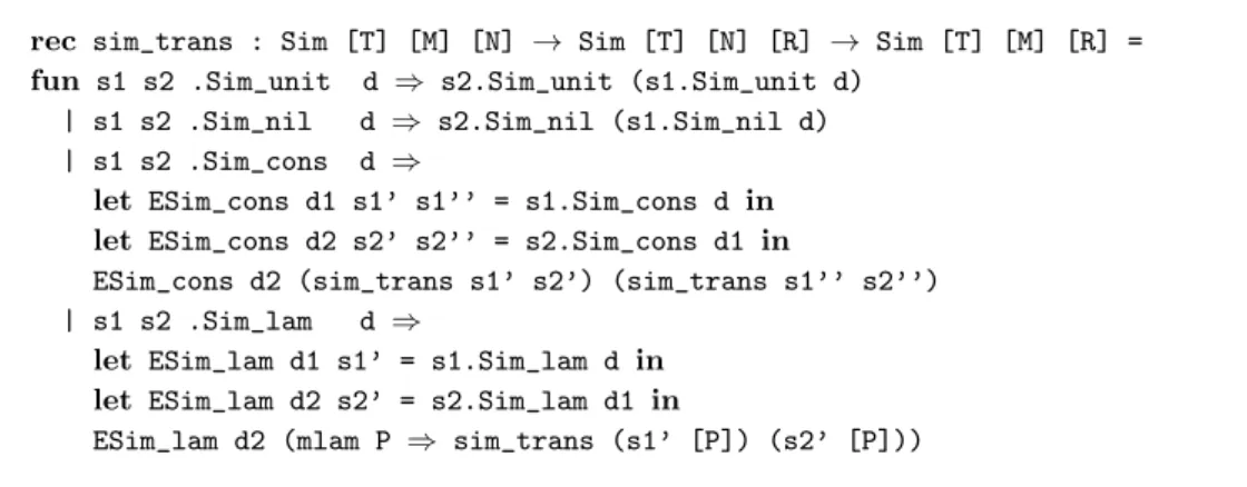
Next, we consider the proof that applicative similarity is transitive: ifSim [T] [M] [N]
andSim [T] [N] [R], thenSim [T] [M] [R](Fig. 8). We comment on a couple of cases:
rec sim_trans : Sim [T] [M] [N] → Sim [T] [N] [R] → Sim [T] [M] [R] =
fun s1 s2 .Sim_unit d ⇒ s2.Sim_unit (s1.Sim_unit d)
| s1 s2 .Sim_nil d ⇒ s2.Sim_nil (s1.Sim_nil d)
| s1 s2 .Sim_cons d ⇒
let ESim_cons d1 s1’ s1’’ = s1.Sim_cons d in
let ESim_cons d2 s2’ s2’’ = s2.Sim_cons d1 in
ESim_cons d2 (sim_trans s1’ s2’) (sim_trans s1’’ s2’’)
| s1 s2 .Sim_lam d ⇒
let ESim_lam d1 s1’ = s1.Sim_lam d in
let ESim_lam d2 s2’ = s2.Sim_lam d1 in
ESim_lam d2 (mlam P ⇒ sim_trans (s1’ [P]) (s2’ [P]))
Fig. 8. Corecursive program showing that similarity is transitive
Observation Sim_unit and T = top. We have the following assumptions: s1: Sim [top
] [M] [N], s2: Sim [top] [N] [R], and d:Eval [M] [unit] and we need to provide
a witness for Eval [R] [unit]. By the observation Sim_unit on s2 (written as the projection s2.Sim_unit), we obtain a function Eval [N] [unit] → Eval [R] [unit]. We pass to it the result ofs1.Sim_unit d.
ObservationSim_lam andT = (arr S S’). We have the assumptions:s1:Sim [arr S T]
[M] [N] ands2:Sim [arr S T] [N] [R]andd:[eval M (lam λx.M’)], and we need to
build a witness forEx_sim_lam [x:term S ` M’] [R]. We first observes1.Sim_lamand
passd:Eval [M] [lam λx.M’]. This hence gives usEx_sim_lam [x:term S ` M’] [N],
which provides us with d1:Eval [N] [lam λx.N’] and s1’:{P:[term S]} Sim [T] [M
’[P]] [N’[P]]. Similarly, we observe s2.Sim_lam passing d1:Eval [N] [lam λx.N’].
Hence we obtainEx_sim_lam [x:term S ` N’] [R], which provides us withd2:Eval
[R] [lam λx.R’]ands2’:{P:[term S]} Sim [T] [N’[P]] [R’[P]]. Building a witness
forEx_sim_lam [x:term S ` M’] [R]requires us to supply a derivationd2:Eval [R]
[lam λx.R’]and a function of type{P:[term S]} Sim [T] [M’[P]] [R’[P]]. We build
3.6. A concrete example of similarity
In this section we show how we can interactively build an actual simulation between two terms, namely that two is simulated by suc one, following the example in (Pitts, 2011). We represent the numbers via Church encodings, where one ≡lamf.lamx. f x,
two≡lamf.lamx. f(f x), andsuc≡lamn.lamx.lamy. x(n x y). We thus want to prove
the following theorem:
rec sim_two_succ_one :
Sim [_] [lam λf.lam λx.app f (app f x)]
[app (lam λn. lam λx. lam λy. app x (app (app n x) y))
(lam λf.lam λx.app f x)]
We will build the proof incrementally, by insertingholes, denoted by?and refining them, analogously to Agda’s methodology. We start with the following program body:
fun .Sim_lam (Ev_val Val_lam) ⇒
ESim_lam (Ev_app (Ev_val Val_lam) (Ev_val Val_lam)) sim_lemma1
wheresim_lemma1is used to abstract over the nested copattern matching:
rec sim_lemma1 : {M:[exp (arr T T)]}
Sim [arr T T]
[lam (λx. app M[] (app M[] x))]
[lam (λy. app M[] (app (app (lam (λf. lam (λw. app f w))) M[]) y))] =
fun [M] .Sim_lam (Ev_val Val_lam) ⇒
ESim_lam (Ev_val Val_lam)
(mlam N ⇒ ?)
Here, the goal has typeSim [_] [app M (app M N)] [app M (app (app (lam (λf. lam
(λw. app f w))) M) N)], which we cannot prove directly using our definition of similarity:
since our evaluation strategy is call-by-name and the metavariable M is not a concrete term, the right-hand side will not reduce. Instead, we use the fact that similarity is a pre-congruence, the main result of this work. We only need property (C3) of Definition 2, which translates to the following lemma.
rec sim_cong_app : Sim [arr S T] [M1] [M2] → Sim [S] [N1] [N2]
→ Sim [T] [app M1 N1] [app M2 N2]
Using this result and reflexivity of similarity, we can thus refine the body ofsim_lemma1:
fun [M] .Sim_lam (Ev_val Val_lam) ⇒
ExSimlam (Ev_val Val_lam)
(mlam N ⇒ sim_cong_app sim_refl ?)
where the current hole has type:
Sim [T] [app M N] [app (app (lam (λu. lam (λw. app u w))) M) N]
Now, we can easily use a derivation of the evaluation of the left-hand side to derive the evaluation of the right-hand side of this similarity as follows:
rec ev1 : Eval [app M N] [V] →
Eval [app (app (lam (λu. lam (λw. app u w))) M) N] [V] =
fun d ⇒ Ev_app (Ev_app (Ev_val Val_lam) (Ev_val Val_lam)) d;
Constructing the above simulation requires us to match on the possible values that
app M Ncan take through the possible observations — in fact all of them as the typeTis
abstract. We then useev1 on the derivations ofEval [app M N] [V] for the givenV and reflexivity when needed.
rec sim_lemma2 : Sim [T] [app M N]
[app (app (lam (λu. lam (λw. app u w))) M) N] =
fun .Sim_lam d ⇒ ESim_lam (ev1 d) (fun [V] ⇒ sim_refl)
| .Sim_unit d ⇒ ev1 d
| .Sim_nil d ⇒ ev1 d
| .Sim_cons d ⇒ ESim_cons (ev1 d) sim_refl sim_refl
Using this lemma, we can complete the body ofsim_lemma1:
fun [M] .Sim_lam (Ev_val Val_lam) ⇒
ExSimlam (Ev_val Val_lam)
(mlam N ⇒ sim_cong_app sim_refl sim_lemma2)
This concludes the proof.
3.7. Defining open similarity using first-class contexts and substitutions
Similarity only relates closed terms. However, in general, we want to be able to reason about similarity of open terms, i.e. terms that depend on a contextγ. InBeluga, we can declare schemas of contexts that classify contexts in the same way that types classify terms and kinds classify types, describing the shape of each declaration in a context. Moreover, we can take advantage of built-in substitutions to relate two contexts. In particular, we can describe grounding substitutions with the type [ ` γ], where the range of the substitution is empty.
We begin by defining the schema of contexts that can occur in our development:
schema ctx = term T;
Here we declare the schemactxthat states that each declaration of a contextγof schema ctxcan only contain variable declarations of typeterm T for some type T. For example, the contextx:term top, y:term (list top)is a valid context of schemactx. On the other hand, a contextx:term unit, a:tpis not.
We can now state open similarity as an inductive type relating well-typed terms in the contextγ. In the kind of the inductive typeOSim, we make the typeTexplicit, but leave
γ implicit. This distinction is reflected in Beluga’s source syntax. We use curly braces
{ } to describe explicit index arguments and round ones ( ) to give type annotations
implicitly.
We can now define open similarity: two terms[γ ` M]and[γ ` N]are openly similar if they are similar for all grounding substitutions σ. Here, we pass γ explicitly toOSimC
inductive Howe: (γ:ctx){T:[tp]}[γ ` term T[] ] → [γ ` term T[] ] → ctype =
| Howe_unit: OSim [top] [γ ` unit] [γ ` M]
→ Howe [top] [γ ` unit] [γ ` M]
| Howe_var : {#p:[γ ` term T[]]} OSim [T] [γ ` #p] [γ ` M]
→ Howe [T] [γ ` #p] [γ ` M]
| Howe_lam : Howe [T] [γ,x:term S[] ` M] [γ,x:term S[] ` N]
→ OSim [arr S T] [γ ` lam λx.N] [γ ` R]
→ Howe [arr S T] [γ ` lam λx.M] [γ ` R]
| Howe_app : Howe [arr S T] [γ ` M] [γ ` M’]
→ Howe [S] [γ ` N] [γ ` N’]
→ OSim [T] [γ ` app M’ N’] [γ ` R]
→ Howe [T] [γ ` app M N] [γ ` R]
...
Fig. 9. The Howe relation
inductive OSim:(γ:ctx){T:[tp]} [γ ` term T[]] → [γ ` term T[]] → ctype =
| OSimC : {γ:ctx}({σ:[ ` γ]} Sim [T] [M[σ]] [N[σ]])
→ OSim [T] [γ ` M] [γ ` N]
We can easily show that open similarity is closed under substitutions by simply com-posing the input substitutionσwith the grounding substitutionσ’.
rec osim_cus : (γ:ctx) (ψ:ctx) {σ:[ψ ` γ]} OSim [T] [γ ` M] [γ ` N]
→ OSim [T] [ψ ` M[σ]] [ψ ` N[σ]] =
fun [ψ ` σ] (OSimC [γ] f) ⇒ OSimC [ψ] (fun [σ’] ⇒ f [σ[σ’]])
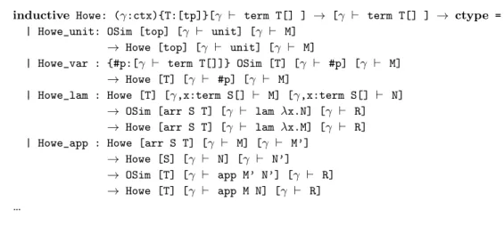
3.8. Defining the Howe relation
The encoding of the Howe relation (see Fig. 9) is, in our view, one of the high points of the formalization: it follows very closely its mathematical formulation, while retaining all the powerful abstractions thatBelugaoffers. This is apparent in the variable case where Beluga’sparameter variables, denoted#p, range over elements from the contextγ. They permit us to precisely characterize when a variable is Howe related to a term M in the given context, while looking remarkably similar to the informal version. The same applies to the lambda abstractions case, where one notes the correct scoping ofM,NandRw.r.t.
γ. The cases forfixandlcasefollow the same principle and we omit them to save space. The structure of the Howe relation makes it trivial to prove that it is a precongruence. We show here the proof in the application case, which is indirectly used for the example of simulation we presented above. The proof of precongruence of similarity in fact follows immediately once we prove equivalent similarity and the Howe relation, see Section 3.10.
rec howe_cong_app : Howe [arr S T] [M1] [M2] → Howe [S] [N1] [N2]
→ Howe [T] [app M1 N1] [app M2 N2] =
inductive Howe_subst: {γ:ctx} (ψ:ctx) {σ1 : [ψ ` γ]} {σ2 : [ψ ` γ]} ctype = | HNil : Howe_subst [] [ψ ` ] [ψ ` ] | HCons : Howe_subst [γ] [ψ ` σ1] [ψ ` σ2] → Howe [T] [ψ ` M] [ψ ` N] → Howe_subst [γ,x:term T[]] [ψ ` σ1, M] [ψ ` σ2, N]
rec howe_subst_wkn : Howe_subst [γ] [ψ ` σ1] [ψ ` σ2]
→ Howe_subst [γ] [ψ,x:term S[] ` σ1[...]] [ψ,x:term S[] ` σ2[...]]
Fig. 10. Howe related substitutions
Using reflexivity and transitivity of open similarity, respectively, we can show reflexivity and semi-transitivity of the candidate relation. We only show the types.
rec howe_refl : (γ:ctx) {M:[γ ` term T[] ]} Howe [T] [γ ` M] [γ ` M]
rec howe_osim_trans : (γ:ctx) Howe [T] [γ ` M] [γ ` N]
→ OSim [T] [γ ` N] [γ ` R]
→ Howe [T] [γ ` M] [γ ` R]
From this it immediately follows that open similarity is a Howe relation.
rec osim_howe:(γ:ctx) OSim [T] [γ ` M] [γ ` N]
→ Howe [T] [γ ` M] [γ ` N] =
fun s ⇒ howe_osim_trans (howe_refl [_ ` _]) s
3.9. Substitutivity of the Howe relation
As remarked in Section 2.2, a crucial point of the proof is showing that the Howe rela-tion is substitutive. Tradirela-tionally, substiturela-tion properties tend to be tedious to prove in proof assistants due to the necessity to reason manually about contexts. Here,Beluga’s contextual abstractions significantly reduces the amount of boilerplate work needed for that proof.
We first encode (Fig. 10) Φ ` σ1 4HΓ σ2 using an inductive type that relates two simultaneous substitutions. The base case relates empty substitutions, written as[ψ `
]. In the inductive case, the substitution[ψ ` σ1, M]and[ψ ` σ2, N] are related, if so are[ψ ` σ1]and[ψ ` σ2]and[ψ ` M]is Howe related to[ψ ` N].
In the subsequent proofs, we rely on the weakening property of simultaneous substi-tutions, namely that weakening preserves Howe-relatedness, see functionhowe_subst_wkn
in Fig. 10. InBeluga, weakening a substitution is simply achieved by composing it with the weakening substitution[...], which has here domainψand rangeψ, x:term S[]. This is supported inBeluga’s theory of simultaneous substitutions (Cave and Pientka, 2013), which internalizes the notions in Fig. 3. The proof ofhowe_subst_wknis done by induction over the predicateHowe_substand by appealing to a special case of substitutivity of Howe
on renamings. In the interest of space, we omit those proofs. In the following, namely in the proof of howe osim (Fig. 12), we will also need the following reflexivity property of
Howe_subst, which holds by a simple induction on substitutions:
rec howe_subst_refl: (γ:ctx)(ψ:ctx){σ:[ψ `γ]}
Howe_subst [γ] [ψ ` σ] [ψ ` σ]
A fragment of the proof of substitutivity inBelugaappears in Fig. 11. We only show here the same two cases we described in the informal proof, together with the variable case, but the remaining cases follow a similar pattern. We make use of the lemmas described above, together with the following additional lemma for the variable case:
rec howe_subst_var : (γ:ctx) (ψ:ctx) Howe [T] [γ ` #p] [γ ` M]
→ Howe_subst [γ] [ψ ` σ1] [ψ ` σ2]
→ Howe [T] [ψ ` #p[σ1]] [ψ ` M[σ2]] =
This is proven by simple induction on the position of the variable in the context which follows the inductive definition ofHowe_subst.
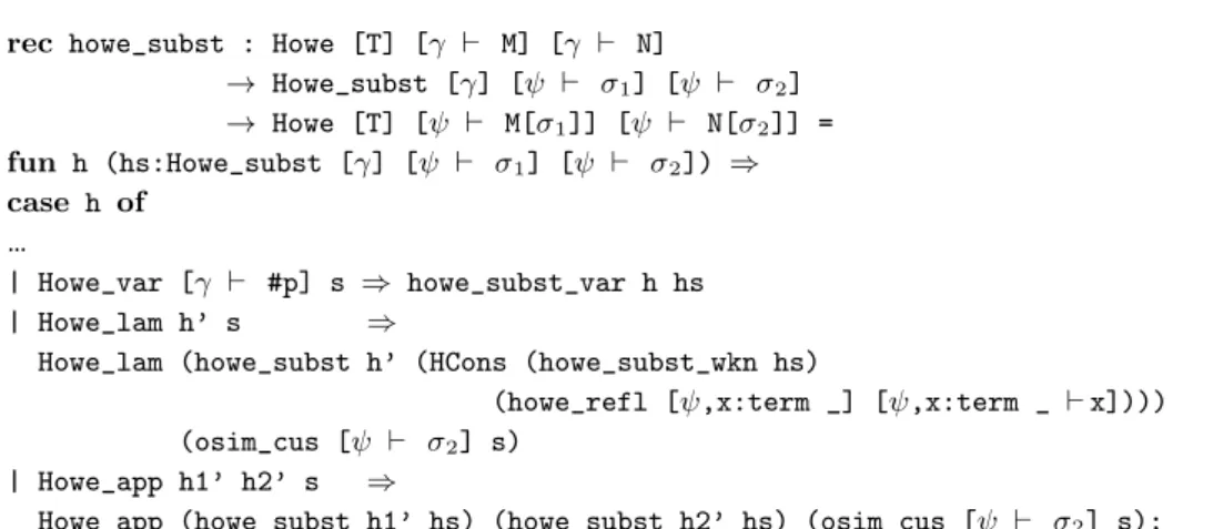
We can see thathowe_subststraightforwardly represents the proof of Lemma 6. What is remarkable in this program with respect to the informal proof is that there are no explicit references to the substitution properties outside of the weakening of the Howe relation on substitutions.
rec howe_subst : Howe [T] [γ ` M] [γ ` N]
→ Howe_subst [γ] [ψ ` σ1] [ψ ` σ2] → Howe [T] [ψ ` M[σ1]] [ψ ` N[σ2]] = fun h (hs:Howe_subst [γ] [ψ ` σ1] [ψ ` σ2]) ⇒ case h of ... | Howe_var [γ ` #p] s ⇒ howe_subst_var h hs | Howe_lam h’ s ⇒
Howe_lam (howe_subst h’ (HCons (howe_subst_wkn hs)
(howe_refl [ψ,x:term _] [ψ,x:term _ `x])))
(osim_cus [ψ ` σ2] s)
| Howe_app h1’ h2’ s ⇒
Howe_app (howe_subst h1’ hs) (howe_subst h2’ hs) (osim_cus [ψ ` σ2] s);
Fig. 11. Substitutivity property of the Howe relation
3.10. Main theorem
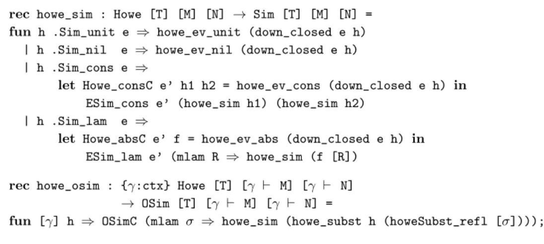
The key lemma in our main theorem is the proof that the Howe relation is downward closed:
rec howe_sim : Howe [T] [M] [N] → Sim [T] [M] [N] =
fun h .Sim_unit e ⇒ howe_ev_unit (down_closed e h)
| h .Sim_nil e ⇒ howe_ev_nil (down_closed e h)
| h .Sim_cons e ⇒
let Howe_consC e’ h1 h2 = howe_ev_cons (down_closed e h) in
ESim_cons e’ (howe_sim h1) (howe_sim h2)
| h .Sim_lam e ⇒
let Howe_absC e’ f = howe_ev_abs (down_closed e h) in
ESim_lam e’ (mlam R ⇒ howe_sim (f [R])
rec howe_osim : {γ:ctx} Howe [T] [γ ` M] [γ ` N]
→ OSim [T] [γ ` M] [γ ` N] =
fun [γ] h ⇒ OSimC (mlam σ ⇒ howe_sim (howe_subst h (howeSubst_refl [σ])));
Fig. 12. The Howe relation is included in open similarity
The proof of this lemma (point 2.1 at page 8) relies on several previous lemmas such as transitivity of closed and open similarity, semi-transitivity and substitutivity of the Howe relation, together with the unfolding of similarity using the observations. The proof is otherwise straightforward but long, and we leave it to the online documentation.
Moving on, we first establish lemmas that mimic the similarity conditions (previous point 2.1). For example: If lamx. m 4Hτ→τ0 n, then n ⇓ lam x. m0 and for every q:τ
we have [q/x]m 4Hτ0 [q/x]m0. Again, as we do not have existential types, we encode
the existence of a term N’ using the inductive types Howe_abs. A fragment of the type signature is as follows:
inductive Howe_abs: [x:term S ` term T[]] → [term (arr S T)] → ctype =
| Howe_absC : Eval [N] [lam λx.N’]
→ ({R:[term T]} Howe [T’] [M’[R]] [N’[R]])
→ HoweAbs [x:term S ` M’] [N];
rec howe_ev_abs : Howe [arr S T] [lam λx.M’] [N]
→ HoweAbs [x:term S ` M’] [N]
We are now ready to prove that the Howe relation coincides with open similarity. We do this by first proving that, in the empty context, the Howe relation is a similarity, then we embed the open version into an open similarity. To do so, we construct out of the input substitutionσfor open similarity a derivation · `σ4HΓ σ by reflexivity. The proofs appear in Fig. 12.
4. Related work
As we mentioned before, Beluga implements indexed copatterns following Thibodeau et al. (2016).Belugais certainly not the only system to feature copatterns, which have been first implemented in MiniAgda (Abel, 2012) in an early form and then in Agda as a
prototype (Abel et al., 2013). Copatterns now show up even in mainstream programming languages such as OCaml (Laforgue and R´egis-Gianas, 2017) as they allow us to integrate elegantly lazy evaluation within an eager language. However,Belugais the only system supporting coinductive reasoning about HOAS representation using copatterns.
The observation paradigm differs from a more traditional approach using lazy con-structors as adopted by Coq (Gim´enez, 1996), in that coinductive types are defined by their elimination rules as opposed to their introduction rules. Coq’s intensional type the-ory offers a strong decidable equational thethe-ory through dependent pattern matching, but loses subject reduction in the presence of coinduction (Oury, 2008). In fact, the change of paradigm to observations was proposed to overcome that very issue with subject re-duction when mixing lazy constructors with dependent case analysis (Abel et al., 2013). Isabelle recently also overhauled (see for example (Biendarra et al., 2017)) their handling of coinduction.
The first HOAS-like formal verification of the congruence of a notion of bisimilarity concerned theπ-calculus (Honsell et al., 2001) and was carried out in Coq using the Weak HOAS approach and instantiating theTheory of Contexts to axiomatizing properties of names. As common in many coinductive developments in Coq, the authors soon ran afoul of the guardedness checker inCofix-style proofs and had to resort to an explicit greatest-fixed point encoding for Strong Late Bisimilairy. Abella’s take on the same issue (Tiu and Miller, 2010) seems preferable; that paper details, among so much more, a proof that similarity is a pre-congruence for the finite π-calculus. The encoding is rather elegant, where all issues involving bindings, names, and substitutions are handled declaratively without explicit side-conditions, thanks to the ∇-quantifier. This style of encoding has been extended in (Chaudhuri et al., 2015) to handle bisimilarity “up-to”. This is achieved via a limited form of quantification on relations that does not have, to our knowledge, a consistency proof yet. The authors do not pursue a proof of congruence in the cited paper.
Recent years have seen much work regarding the formalization of process calculi, in particular using Nominal Isabelle. We do not have the space to discuss this line of work in detail but simply cite some of the many contributions from Parrow and his asso-ciates (Bengtson and Parrow, 2009; Parrow et al., 2014; Bengtson et al., 2016) about various versions of the π/ψ-calculus and their congruence properties, proven without resorting to the Howe’s proof strategy.
Encoding bisimilarity in the λ-calculus, in particular via Howe’s method, brings in additional challenges, as we have seen. We are aware of several formalizations through the years:
1. In (Ambler and Crole, 1999) the authors verify in Isabelle/HOL 98 the same result of the present paper and a bit more (they also show that similarity coincides with contextual pre-order) for PCFL using de Bruijn indexes as an encoding techniques for binders. The development, for the congruence part, consists of around 160 lem-mas/theorems, and it confirms a common belief about (standard) concrete syntax approaches: doable, but very hard-going;