A neutron noise solver based on a discrete ordinates method

(1)

THESIS FOR THE DEGREE OF LICENTIATE OF ENGINEERING

CTH-NT-341 February 2020

A neutron noise solver based on a discrete ordinates method

HUAIQIAN YI

Division of Subatomic, High Energy and Plasma Physics Department of Physics

CHALMERS UNIVERSITY OF TECHNOLOGY Gothenburg, Sweden 2020

(2)

A neutron noise solver based on a discrete ordinates method HUAIQIAN YI

Technical report no CTH-NT-341

Chalmers University of Technology SE-412 96 Gothenburg

Sweden

Telephone + 46 (0)31-772 1000

Chalmers Digital Print Gothenburg, Sweden 2020

(3)

I

A neutron noise solver based on a discrete ordinates method HUAIQIAN YI

Chalmers University of Technology

Abstract

A neutron noise transport modelling tool is presented in this thesis. The simulator allows to determine the static solution of a critical system and the neutron noise induced by a prescribed perturbation of the critical system. The simulator is based on the neutron balance equations in the frequency domain and for two-dimensional systems. The discrete ordinates method is used for the angular discretization and the diamond finite difference method for the treatment of the spatial variable. The energy dependence is modelled with two neutron energy groups. The conventional inner-outer iterative scheme is employed for solving the discretized neutron transport equations. For the acceleration of the iterative scheme, the diffusion synthetic acceleration is implemented.

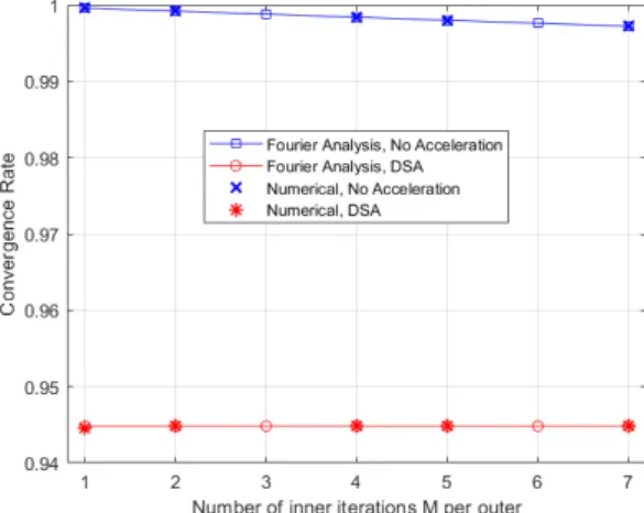
The convergence rate of the accelerated and unaccelerated versions of the simulator is studied for the case of a perturbed infinite homogeneous system. The theoretical behavior predicted by the Fourier convergence analysis agrees well with the numerical performance of the simulator. The diffusion synthetic acceleration decreases significantly the number of numerical iterations, but its convergence rate is still slow, especially for perturbations at low frequencies.

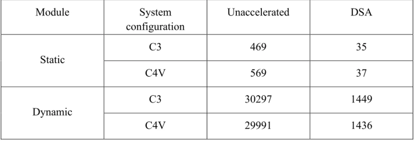
The simulator is further tested on neutron noise problems in more realistic, heterogeneous systems and compared with the diffusion-based solver. The diffusion synthetic acceleration leads to a reduction of the computational burden by a factor of 20. In addition, the simulator shows results that are consistent with the diffusion-based approximation. However, discrepancies are found because of the local effects of the neutron noise source and the strong variations of material properties in the system, which are expected to be better reproduced by a higher-order transport method such as the one used in the new solver.

Keywords: Neutron noise, nuclear reactor modelling, deterministic neutron transport methods, discrete ordinates, diffusion synthetic acceleration, convergence analysis

(4)

(5)

III

List of Publications

Papers included in the thesis: PAPER I

H. Yi, P. Vinai and C. Demazière, “A discrete ordinates solver with diffusion synthetic acceleration for simulations of 2-D and 2-energy group neutron noise problems,” International Conference on Mathematics and Computational Methods applied to Nuclear Science and Engineering, M&C 2019, Portland, Oregon USA, August 25-29, 2019.

https://doi.org/10.5281/zenodo.3567612 PAPER II

A. Mylonakis, H. Yi, P. Vinai and C. Demazière, “Neutron noise simulations in a heterogeneous system: A comparison between a diffusion-based and a discrete ordinates solver,” International Conference on Mathematics and Computational Methods applied to Nuclear Science and Engineering, M&C 2019, Portland, Oregon USA, August 25-29, 2019.

https://doi.org/10.5281/zenodo.3567577

The author’s contribution to the included papers:

PAPER I: Huaiqian Yi (HY) developed the transport neutron noise code, performed the theoretical and the simulation work for the convergence analysis of the solver, interpreted the results, and wrote the paper together with the co-authors.

PAPER II: HY developed the model for the discrete ordinates solver, performed the simulations with the discrete ordinates solver, prepared the plots about the comparison between the discrete ordinates solver and CORE SIM, contributed to the interpretation of the results.

Papers not related to the thesis subject and not included in the thesis:

H. Yi, C. Demazière, P. Vinai and J. Leppänen, “Development and Test of a Hybrid Probabilistic-Deterministic Framework Based on The Interface Current Method,” International Conference on Mathematics and Computational Methods applied to Nuclear Science and Engineering, M&C 2019, Portland, Oregon USA, August 25-29, 2019.

(6)

(7)

V

Acknowledgements

First and foremost, I would like to thank my supervisor Assoc. Prof. Paolo Vinai for his guidance in my daily work and in the preparation this thesis. The works could not be accomplished and the thesis would not be close to its final state without his enormous help and support with great patience and dedication.

I would also like to thank my co-supervisor and examiner Prof. Christophe Demazière for insightful discussions and suggestions that helped to improve my work and the thesis.

Special thanks to Dr. Antonios Mylonakis for all the discussions we had in the office which helped me to overcome obstacles I encountered.

Lots of thanks to my family for their support and care throughout the whole time of my studies. The research leading to these results has received funding from the Euratom research and training program 2014-2018 under grant agreement No. 754316. The financial support is gratefully appreciated.

(8)

(9)

VII

Chapter 1 Introduction

The general background and the motivations of the work reported in this thesis are discussed together with the structure of the thesis.

1.1 Reactor neutron noise, and core monitoring and

diagnostics

In nuclear reactors, the neutron flux is an important quantity to monitor, from an operational and safety viewpoint, since it is proportional to the reactor power output. Therefore, nuclear reactors are equipped with detectors for neutron flux measurements. The signals of these detectors show small fluctuations around the expected mean values, even under normal, steady state operating conditions. Such fluctuations are referred to as reactor neutron noise. In reactors operating at a high-power-level, this phenomenon is driven by perturbations such as vibrations of reactor components, disturbances in the operational conditions, etc. From the analysis of the neutron noise it is possible to obtain information about the dynamic properties of a reactor, identify anomalous patterns and, if necessary, take appropriate actions before dangerous situations arise [1, 2, 3].

Figure 1.1 Illustration of using reactor neutron noise for core monitoring and diagnostics. [3] The use of neutron noise analysis for core monitoring and diagnostics requires the modelling of the reactor transfer function. The function describes the response of the neutron flux in the core induced by any possible perturbation. Its inversion allows to identify and locate the noise source from the measured neutron noise. Given the complexity of a reactor system, this task cannot be performed in an analytical manner, so numerical methods must be used.

(12)

Chapter 1 Introduction

2

Most of the past work in the modelling of the transfer function relies on neutron diffusion theory, e.g. [4]. The advantage of this approach is that neutron noise problems in relatively large systems can be simulated without heavy computational efforts. Nevertheless, recent efforts also focus on higher-order deterministic [5] or stochastic [6, 7, 8] methods for solving the transport neutron noise equation. Although these methods are more computationally expensive, they can provide more detailed results and be used to assess the limitations of the diffusion approximation for neutron noise applications.

In the current thesis the first steps in the development of a higher-order transport solver for neutron noise simulations are presented. This research activity is part of the CORTEX project which aims to investigate reactor core monitoring and diagnostic techniques based on the analysis of neutron noise [2] and is supported by EU within the framework HORIZON 2020 – EURATOM.

1.2 Structure of the thesis

The thesis is built from the contents of Paper I and Paper II and is structured as follows. In Chapter 2, the multi-energy-group neutron noise equations in the frequency domain are derived. In Chapter 3, the numerical algorithms used to solve the neutron noise equation in the case of two-energy groups and two-dimensional geometry, are described. In Chapter 4, the analysis of the convergence of the solver and the comparison with a diffusion-based solution for a two-dimensional heterogeneous system with a localized neutron noise source are discussed. In Chapter 5, conclusions and an outlook for future work are provided.

(13)

Chapter 2 Multi-energy-group neutron noise equation

3

Chapter 2 Multi-energy-group neutron noise equation

The time-dependent neutron balance equations used to describe nuclear reactor kinetics are introduced in Section 2.1. The transport neutron noise equation in the frequency domain is derived in Section 2.2. The solution of the neutron noise equations in the frequency domain is an advantageous strategy since it avoids expensive time-dependent simulations and requires only calculations for the frequency at which the neutron noise sources fluctuate.

2.1 Neutron kinetics equations

In a nuclear reactor, a fraction of the neutrons released from the fission reactions appears with a delay of seconds to minutes because of the beta decay of some fission products (the so-called precursors of delayed neutrons). Therefore, the modelling of the time-dependent behaviour of a reactor consists of a balance equation for the neutron density coupled to balance equations for the precursors of delayed neutrons. The precursors of delayed neutrons are usually grouped into a number of families according to their decay constants and a balance equation is given for each family. Then the neutron kinetics equations (with scattering treated as isotropic) reads, in a macroscopic sense, as:

�_𝑣𝑣₍_𝑟𝑟⃗1_,_𝐸𝐸₎_{𝜕𝜕𝜕𝜕}𝜕𝜕 +𝛺𝛺� ∙ 𝛻𝛻+𝛴𝛴𝑡𝑡(𝑟𝑟⃗,𝐸𝐸,𝜕𝜕)� 𝜓𝜓�𝑟𝑟⃗,𝛺𝛺�,𝐸𝐸,𝜕𝜕� =₄1_{𝜋𝜋 � 𝛴𝛴}𝑠𝑠(𝑟𝑟⃗,𝐸𝐸′→ 𝐸𝐸,𝜕𝜕)𝜙𝜙(𝑟𝑟⃗,𝐸𝐸′,𝜕𝜕)𝑑𝑑𝐸𝐸′ + 1 4𝜋𝜋𝑘𝑘𝑒𝑒𝑒𝑒𝑒𝑒�𝜒𝜒𝑝𝑝(𝑟𝑟⃗,𝐸𝐸)� �_𝑞𝑞 1− 𝛽𝛽𝑞𝑞(𝑟𝑟⃗)�� 𝜈𝜈𝛴𝛴𝑒𝑒(𝑟𝑟⃗,𝐸𝐸 ′_,_𝜕𝜕₎_𝜙𝜙₍_𝑟𝑟⃗_,_𝐸𝐸′_,_𝜕𝜕₎_{𝑑𝑑𝐸𝐸}′₊_{� 𝜒𝜒} 𝑑𝑑,𝑞𝑞(𝑟𝑟⃗,𝐸𝐸)𝜆𝜆𝑞𝑞𝐶𝐶𝑞𝑞(𝑟𝑟⃗,𝜕𝜕) 𝑞𝑞 �( 2. 1 ) and 𝜕𝜕𝐶𝐶𝑞𝑞(𝑟𝑟⃗,𝜕𝜕) 𝜕𝜕𝜕𝜕 = 𝛽𝛽𝑞𝑞(𝑟𝑟⃗)� 𝜈𝜈𝛴𝛴𝑒𝑒(𝑟𝑟⃗,𝐸𝐸′,𝜕𝜕)𝜙𝜙(𝑟𝑟⃗,𝐸𝐸′,𝜕𝜕)𝑑𝑑𝐸𝐸′− 𝜆𝜆𝑞𝑞𝐶𝐶𝑞𝑞(𝑟𝑟⃗,𝜕𝜕),𝑤𝑤𝑤𝑤𝜕𝜕ℎ𝑞𝑞= 1, … ,𝑄𝑄 ( 2. 2 )

Eq. (2.1) is the balance equation for the neutrons and is written in terms of the angular flux

𝜓𝜓�𝑟𝑟⃗,𝛺𝛺�,𝐸𝐸,𝜕𝜕�, which depends on the space vector 𝑟𝑟⃗, the angular direction Ω�, the energy 𝐸𝐸 and the time 𝜕𝜕. On the left-hand side, the three terms represent, respectively, the time variation of the neutron density, the streaming of neutrons and the disappearance of neutrons in the unit phase space. The right-hand side contains three source terms related to scattering, prompt and delayed neutrons emitted from fission reactions, respectively. For the scattering and prompt fission contributions, the scalar flux 𝜙𝜙(𝑟𝑟⃗,𝐸𝐸,𝜕𝜕) estimated from the integration of the angular flux over all the angular directions, is used. In this equation, isotropy for the directions of the neutrons emitted from both prompt and delayed fission events are also assumed. The

(14)

4

contribution from the fission reactions is normalized using the effective multiplication factor

𝑘𝑘𝑒𝑒𝑒𝑒𝑒𝑒, since in the current work only perturbations in critical systems are considered.

Eq. (2.2) gives the rate of change in the concentration 𝐶𝐶𝑞𝑞(𝑟𝑟⃗,𝜕𝜕) of the 𝑞𝑞-th family of delayed

neutron precursors as the difference between the precursors created by fission and the precursors disappearing because of decay. This balance is equivalent to the balance of delayed neutrons since each precursor ultimately emits 1 delayed neutron.

In order to simplify the problem, the energy dependence is treated with the multi-group formalism. The range of all possible neutron energy is divided into G energy bins as:

[𝐸𝐸𝑚𝑚𝑚𝑚𝑚𝑚:𝐸𝐸𝑚𝑚𝑚𝑚𝑚𝑚] =��𝐸𝐸𝑔𝑔:𝐸𝐸𝑔𝑔−1� 1

𝑔𝑔=𝐺𝐺

( 2. 3 ) where the first group (𝑔𝑔=1) has the neutrons with highest energies and the lowest energy neutrons belong to the last group (𝑔𝑔= 𝐺𝐺). Eqs. (2.1) and (2.2) are integrated over the predefined energy bins and the following multi-group kinetics equations are obtained:

� 1 𝑣𝑣𝑔𝑔(𝑟𝑟⃗) 𝜕𝜕 𝜕𝜕𝜕𝜕+𝛺𝛺� ∙ 𝛻𝛻+𝛴𝛴𝑡𝑡,𝑔𝑔(𝑟𝑟⃗,𝜕𝜕)� 𝜓𝜓𝑔𝑔�𝑟𝑟⃗,𝛺𝛺�,𝜕𝜕� = ₄1_{𝜋𝜋 � 𝛴𝛴}_𝑠𝑠_,_𝑔𝑔′_→𝑔𝑔(𝑟𝑟⃗,𝜕𝜕)𝜙𝜙_𝑔𝑔′(𝑟𝑟⃗,𝜕𝜕) 𝑔𝑔′ +₄_{𝜋𝜋𝑘𝑘}1 𝑒𝑒𝑒𝑒𝑒𝑒�𝜒𝜒𝑝𝑝,𝑔𝑔(𝑟𝑟⃗)� �_𝑞𝑞 1− 𝛽𝛽𝑞𝑞(𝑟𝑟⃗)�� 𝜈𝜈𝛴𝛴_𝑔𝑔_′ 𝑒𝑒,𝑔𝑔′(𝑟𝑟⃗,𝜕𝜕)𝜙𝜙𝑔𝑔′(𝑟𝑟⃗,𝜕𝜕)+� 𝜒𝜒_𝑞𝑞 𝑑𝑑,𝑞𝑞,𝑔𝑔(𝑟𝑟⃗)𝜆𝜆𝑞𝑞𝐶𝐶𝑞𝑞(𝑟𝑟⃗,𝜕𝜕)� ( 2. 4 ) and 𝜕𝜕𝐶𝐶𝑞𝑞(𝑟𝑟⃗,𝜕𝜕) 𝜕𝜕𝜕𝜕 =𝛽𝛽𝑞𝑞(𝑟𝑟⃗)� 𝜈𝜈𝛴𝛴𝑒𝑒,𝑔𝑔′(𝑟𝑟⃗,𝜕𝜕)𝜙𝜙𝑔𝑔′(𝑟𝑟⃗,𝜕𝜕) 𝑔𝑔′ − 𝜆𝜆𝑞𝑞𝐶𝐶𝑞𝑞(𝑟𝑟⃗,𝜕𝜕) ( 2. 5 )

Setting the time derivatives in Eqs. (2.4) and (2.5) equal to zero, leads to the static equation:

�𝛺𝛺� ∙ 𝛻𝛻+𝛴𝛴𝑡𝑡,𝑔𝑔,0(𝑟𝑟⃗)�𝜓𝜓𝑔𝑔,0�𝑟𝑟⃗,𝛺𝛺��= ₄1_{𝜋𝜋 � 𝛴𝛴}𝑠𝑠,𝑔𝑔′→𝑔𝑔,0(𝑟𝑟⃗)𝜙𝜙𝑔𝑔′,0(𝑟𝑟⃗) 𝑔𝑔′

+₄_{𝜋𝜋𝑘𝑘}1

𝑒𝑒𝑒𝑒𝑒𝑒�𝜒𝜒𝑝𝑝,𝑔𝑔(𝑟𝑟⃗)� �_𝑞𝑞 1− 𝛽𝛽𝑞𝑞(𝑟𝑟⃗)�+� 𝜒𝜒_𝑞𝑞 𝑑𝑑,𝑞𝑞,𝑔𝑔(𝑟𝑟⃗)𝛽𝛽𝑞𝑞(𝑟𝑟⃗)� � 𝜈𝜈𝛴𝛴_𝑔𝑔_′ 𝑒𝑒,𝑔𝑔′,0(𝑟𝑟⃗)𝜙𝜙𝑔𝑔′,0(𝑟𝑟⃗) ( 2. 6 )

where the static quantities are denoted with the subscript “0”. Eq. (2.6) corresponds to an eigenvalue problem whose solution gives both the eigenvalue 𝑘𝑘𝑒𝑒𝑒𝑒𝑒𝑒 and the static neutron

(15)

5

2.2 Frequency domain transport neutron noise equation

The derivation of the transport neutron noise equation in the frequency domain follows a standard procedure used already in other works, e.g. [1, 4].

A critical system is assumed to be affected by a perturbation that can be described by a small, stationary fluctuation of the macroscopic neutron cross-sections around their mean values. The perturbation induces small fluctuations of the neutron flux and of the delayed neutron precursor concentrations. These quantities then can be written as the sum of a static mean value and a fluctuating part, such as:

𝑋𝑋(𝑟𝑟⃗,𝜕𝜕) =𝑋𝑋0(𝑟𝑟⃗) +𝛿𝛿𝑋𝑋(𝑟𝑟⃗,𝜕𝜕) ( 2. 7 )

Eq. (2.7) is used for the macroscopic cross-sections, the delayed neutron precursor concentrations, the angular and the scalar neutron flux, into the neutron kinetics equations (2.4) and (2.5). The second order perturbation terms are neglected because the fluctuations are small and linear theory can be applied. The static equation (2.6) is subtracted and a temporal Fourier transform is performed. The resulting equation is the transport neutron noise equation in the frequency domain and reads as:

�𝛺𝛺� ∙ 𝛻𝛻+𝛴𝛴𝑡𝑡,𝑔𝑔,0(𝑟𝑟⃗) +_𝑣𝑣𝑤𝑤𝑖𝑖 𝑔𝑔(𝑟𝑟⃗)� 𝛿𝛿𝜓𝜓𝑔𝑔�𝑟𝑟⃗,𝛺𝛺�,𝑖𝑖�= 1 4𝜋𝜋 � 𝛴𝛴_𝑔𝑔′ 𝑠𝑠,𝑔𝑔′→𝑔𝑔,0(𝑟𝑟⃗)𝛿𝛿𝜙𝜙𝑔𝑔′(𝑟𝑟⃗,𝑖𝑖) +₄_{𝜋𝜋𝑘𝑘}1 𝑒𝑒𝑒𝑒𝑒𝑒�𝜒𝜒𝑝𝑝,𝑔𝑔(𝑟𝑟⃗)� �_𝑞𝑞 1− 𝛽𝛽𝑞𝑞(𝑟𝑟⃗)�+� 𝜒𝜒𝑑𝑑,𝑞𝑞,𝑔𝑔(𝑟𝑟⃗) 𝜆𝜆𝑞𝑞𝛽𝛽𝑞𝑞(𝑟𝑟⃗) 𝑤𝑤𝑖𝑖+𝜆𝜆𝑞𝑞 𝑞𝑞 � � 𝜈𝜈𝛴𝛴𝑒𝑒,𝑔𝑔′,0(𝑟𝑟⃗)𝛿𝛿𝜙𝜙𝑔𝑔′(𝑟𝑟⃗,𝑖𝑖) 𝑔𝑔′ +𝑆𝑆𝑔𝑔�𝑟𝑟⃗,𝛺𝛺�,𝑖𝑖� ( 2. 8 )

where the noise source 𝑆𝑆𝑔𝑔�𝑟𝑟⃗,𝛺𝛺�,𝑖𝑖� has the following expression:

Sg�𝑟𝑟⃗,𝛺𝛺�,𝑖𝑖�=−δ𝛴𝛴𝑡𝑡,𝑔𝑔(𝑟𝑟⃗,𝑖𝑖)𝜓𝜓𝑔𝑔,0�𝑟𝑟⃗,𝛺𝛺��+₄1_{𝜋𝜋 � δ𝛴𝛴}𝑠𝑠,𝑔𝑔′_→𝑔𝑔(𝑟𝑟⃗,𝑖𝑖)𝜙𝜙_𝑔𝑔′_,₀(𝑟𝑟⃗) 𝑔𝑔′ +₄_{𝜋𝜋𝑘𝑘}1 𝑒𝑒𝑒𝑒𝑒𝑒�𝜒𝜒𝑝𝑝,𝑔𝑔(𝑟𝑟⃗)� �_𝑞𝑞 1− 𝛽𝛽𝑞𝑞(𝑟𝑟⃗)�+� 𝜒𝜒𝑑𝑑,𝑞𝑞,𝑔𝑔(𝑟𝑟⃗) 𝜆𝜆𝑞𝑞𝛽𝛽𝑞𝑞(𝑟𝑟⃗) 𝑤𝑤𝑖𝑖+𝜆𝜆𝑞𝑞 𝑞𝑞 � � 𝜈𝜈𝛿𝛿𝛴𝛴𝑒𝑒,𝑔𝑔′(𝑟𝑟⃗,𝑖𝑖)𝜙𝜙_𝑔𝑔′_,₀(𝑟𝑟⃗) 𝑔𝑔′ ( 2. 9 ) In the neutron noise equations, 𝑤𝑤 is the imaginary unit and 𝑖𝑖 = 2𝜋𝜋𝜋𝜋 is the angular frequency of the perturbation. As can be seen in Eqs. (2.8) and (2.9), 𝑘𝑘𝑒𝑒𝑒𝑒𝑒𝑒 and the static neutron fluxes are

needed; therefore Eq. (2.6) must be first solved. Eq. (2.8) represents a fixed source problem with the fixed 𝑘𝑘𝑒𝑒𝑒𝑒𝑒𝑒 obtained from the static problem. The solution to the noise problem

provides the angular neutron noise 𝛿𝛿𝜓𝜓𝑔𝑔 and the scalar neutron noise δ𝜙𝜙𝑔𝑔 as complex numbers.

Combining the real and imaginary parts of these quantities, amplitude and phase of the angular and scalar neutron noise can be estimated.

(16)

(17)

Chapter 3 Neutron noise solver

7

Chapter 3 Neutron noise solver

The computational methods and algorithms applied to solve the neutron noise equation are presented. In Section 3.1, the overall calculation scheme of the solver is provided. In Section 3.2, the discrete ordinates method for the angular discretization and the diamond finite difference method for the spatial discretization are introduced. In Section 3.3, the transport sweeps and the iterative procedure for solving the multigroup transport equations are discussed. In Section 3.4, the diffusion synthetic acceleration method is described.

3.1 Calculation scheme

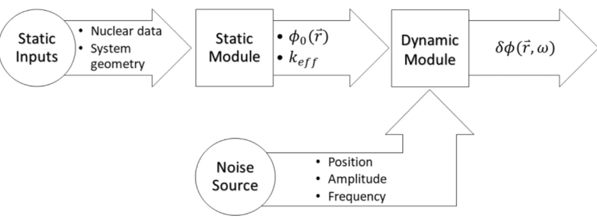
As shown in Section 2.2, the solution of the neutron noise equations in the frequency domain needs the value of 𝑘𝑘𝑒𝑒𝑒𝑒𝑒𝑒 and the static fluxes. Therefore, the solver that is under development in

this project, consists of a static and a dynamic module (see Fig. 3.1). The static module first solves the eigenvalue problem represented by Eq. (2.6) so that the space dependent static angular and scalar fluxes and the effective multiplication factor 𝑘𝑘𝑒𝑒𝑒𝑒𝑒𝑒 are estimated. The

dynamic module then solves Eq. (2.8), provided with the inputs from the static module and the position, amplitude and frequency of the fluctuating perturbation. The two modules are independent, so the first step in the calculation does not need to be repeated for problems with the same static configuration but different neutron noise sources.

(18)

8

3.2 Angular and spatial differencing schemes

When solving numerically the problem, the equations are discretized with respect to the independent variables. The energy discretization is discussed in Section 2.1 and leads to the multi-energy-group equations. In addition, the discrete ordinates method and the diamond finite difference method are used for the angular variable Ω� and the spatial variable 𝑟𝑟⃗, respectively. Consistently with the neutron noise solver presented in this thesis, the discussions are hereinafter based on two-dimensional cases.

3.2.1 Discrete ordinates method

In this work, a discrete ordinate method is applied to the angular discretization of Eqs. (2.6) and (2.8). The discrete ordinates (SN) method has been widely used in the nuclear community for solving the neutron transport equation because it is acknowledged for its simplicity in the derivation process, and for its good computational efficiency while avoiding excessive computer memory consumption [9].

The angular variable 𝛺𝛺� is expressed by the direction cosines. In the 2-D case, it is then given as:

𝛺𝛺� =𝛺𝛺��𝛺𝛺�𝑚𝑚,𝛺𝛺�𝑦𝑦�= 𝛺𝛺��𝛺𝛺� ∙ 𝑒𝑒̂𝑚𝑚,𝛺𝛺� ∙ 𝑒𝑒̂𝑦𝑦�= 𝛺𝛺�(𝜇𝜇,𝜂𝜂) (3. 1)

where 𝑒𝑒̂𝑚𝑚 and 𝑒𝑒̂𝑦𝑦 are the unit vectors in the positive direction of the two axes of the cartesian

coordinate system. In the SN method, the transport equations are evaluated along a fixed number of discrete angular directions.

Similar to the static case, the transport neutron noise equation for the generic discrete angular direction 𝛺𝛺�𝑚𝑚 =𝛺𝛺�(𝜇𝜇𝑚𝑚,𝜂𝜂𝑚𝑚) can thus be written as:

�𝜇𝜇𝑚𝑚_{𝜕𝜕𝜕𝜕}𝜕𝜕 +𝜂𝜂𝑚𝑚_{𝜕𝜕𝜕𝜕}𝜕𝜕 +𝛴𝛴𝑡𝑡,𝑔𝑔,0(𝑟𝑟⃗) +_𝑣𝑣𝑤𝑤𝑖𝑖 𝑔𝑔(𝑟𝑟⃗)� 𝛿𝛿𝜓𝜓𝑔𝑔,𝑚𝑚(𝑟𝑟⃗,𝑖𝑖) = 1 2𝜋𝜋 � 𝛴𝛴𝑠𝑠,𝑔𝑔′→𝑔𝑔,0(𝑟𝑟⃗)𝛿𝛿𝜙𝜙𝑔𝑔′(𝑟𝑟⃗,𝑖𝑖) 𝑔𝑔′ +₂_{𝜋𝜋𝑘𝑘}1 𝑒𝑒𝑒𝑒𝑒𝑒�𝜒𝜒𝑝𝑝,𝑔𝑔(𝑟𝑟⃗)� �_𝑞𝑞 1− 𝛽𝛽𝑞𝑞(𝑟𝑟⃗)�+� 𝜒𝜒𝑑𝑑,𝑞𝑞,𝑔𝑔(𝑟𝑟⃗) 𝜆𝜆𝑞𝑞𝛽𝛽𝑞𝑞(𝑟𝑟⃗) 𝑤𝑤𝑖𝑖+𝜆𝜆𝑞𝑞 𝑞𝑞 � � 𝜈𝜈𝛴𝛴𝑒𝑒,𝑔𝑔′_,₀(𝑟𝑟⃗)𝛿𝛿𝜙𝜙_𝑔𝑔′(𝑟𝑟⃗,𝑖𝑖) 𝑔𝑔′ +𝑆𝑆𝑔𝑔,𝑚𝑚(𝑟𝑟⃗,𝑖𝑖) (3. 2)

with the noise source given as:

𝑆𝑆𝑔𝑔,𝑚𝑚(𝑟𝑟⃗,𝑖𝑖) =−δ𝛴𝛴𝑡𝑡,𝑔𝑔(𝑟𝑟⃗,𝑖𝑖)𝜓𝜓𝑔𝑔,𝑚𝑚,0(𝑟𝑟⃗) +₂1_{𝜋𝜋 � δ𝛴𝛴}𝑠𝑠,𝑔𝑔′_→𝑔𝑔(𝑟𝑟⃗,𝑖𝑖)𝜙𝜙_𝑔𝑔′_,₀(𝑟𝑟⃗) 𝑔𝑔′ +₂_{𝜋𝜋𝑘𝑘}1 𝑒𝑒𝑒𝑒𝑒𝑒�𝜒𝜒𝑝𝑝,𝑔𝑔(𝑟𝑟⃗)� �_𝑞𝑞 1− 𝛽𝛽𝑞𝑞(𝑟𝑟⃗)�+� 𝜒𝜒𝑑𝑑,𝑞𝑞,𝑔𝑔(𝑟𝑟⃗) 𝜆𝜆𝑞𝑞𝛽𝛽𝑞𝑞(𝑟𝑟⃗) 𝑤𝑤𝑖𝑖+𝜆𝜆𝑞𝑞 𝑞𝑞 � � 𝜈𝜈𝛿𝛿𝛴𝛴_𝑒𝑒_,_𝑔𝑔′(𝑟𝑟⃗,𝑖𝑖)𝜙𝜙_𝑔𝑔′_,₀(𝑟𝑟⃗) 𝑔𝑔′ (3. 3) In Eq. (3.2) the notation 𝛿𝛿𝜓𝜓𝑔𝑔,𝑚𝑚(𝑟𝑟⃗,𝑖𝑖) =𝛿𝛿𝜓𝜓𝑔𝑔�𝑟𝑟��⃗ 𝛺𝛺�, 𝑚𝑚,𝑖𝑖� is used to represent the angular neutron

noise for the 𝑛𝑛-th discrete angular direction. The scalar neutron noise is calculated with a quadrature formula that approximates the angle integration:

(19)

Chapter 3 Neutron noise solver 9 𝛿𝛿𝜙𝜙𝑔𝑔(𝑟𝑟⃗,𝑖𝑖) =𝜋𝜋₂� 𝑤𝑤𝑚𝑚𝛿𝛿𝜓𝜓𝑔𝑔,𝑚𝑚(𝑟𝑟⃗,𝑖𝑖) 𝑁𝑁0 𝑚𝑚=1 (3. 4) The parameter 𝑁𝑁0 is the total number of discrete angular directions and the weights 𝑤𝑤𝑚𝑚 are

normalized according to the following relationship:

� 𝑤𝑤𝑚𝑚 𝑁𝑁0

𝑚𝑚=1

= 4 (3. 5)

The direction cosines and their corresponding weights can be determined with different quadrature sets. The widely applied level symmetric quadrature set (𝐿𝐿𝑄𝑄𝑁𝑁) is chosen in this

work. Using the 𝐿𝐿𝑄𝑄𝑁𝑁 sets in two-dimensional geometry, the discrete ordinates approximation

of order 𝑁𝑁 has (𝑁𝑁+ 2)𝑁𝑁/2 discrete directions. The details of the level symmetric method can be found, e.g., in [9].

One major drawback of the SN method applied to static calculations is the so called “ray effects”. Unphysical results may be generated if a low order SN approximation is used to solve problems defined in a highly absorbent media with localized source. This effect is also observed in the neutron noise problems that are discussed in Chapter 4. In this work, the most straightforward remedy, where the number of discrete ordinates is increased, is tested and it is shown to improve the results.

3.2.2 Diamond finite difference scheme

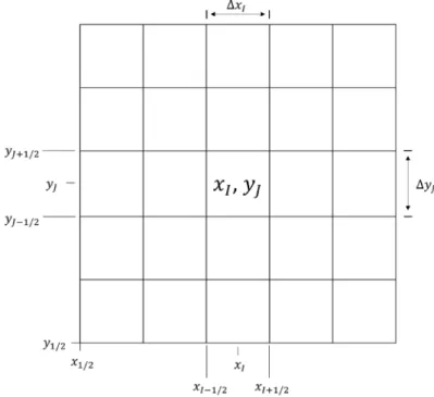
The discretization of the spatial variable is based on the diamond finite difference scheme. The method has been largely applied to the static equations [9]. Then the discussion is focused on the neutron noise equations.

(20)

10

A 2-dimensional domain is considered in the 𝜕𝜕 − 𝜕𝜕 plane. As shown in Figure 3.2, the domain is divided into cells bounded by the coordinates 𝜕𝜕1/2, 𝜕𝜕3/2,⋯,𝜕𝜕𝐼𝐼𝑚𝑚𝑚𝑚𝑚𝑚+/2 in the direction 𝜕𝜕 and

𝜕𝜕1/2, 𝜕𝜕3/2,⋯,𝜕𝜕𝐽𝐽𝑚𝑚𝑚𝑚𝑚𝑚+/2 in the direction 𝜕𝜕. Each cell thus are rectangles with width ∆𝜕𝜕𝐼𝐼 =

𝜕𝜕𝐼𝐼+1/2− 𝜕𝜕𝐼𝐼−1/2 and ∆𝜕𝜕𝐽𝐽 =𝜕𝜕𝐽𝐽+1/2− 𝜕𝜕𝐽𝐽−1/2. In each cell, the system parameters take constant

values and change only at the boundaries of the cells denoted by the half-integers. By integrating Eq. (3.2) over the generic cell (𝐼𝐼, 𝐽𝐽), the following relationship is obtained:

𝜇𝜇𝑚𝑚 ∆𝜕𝜕𝐼𝐼�𝛿𝛿𝜓𝜓𝑔𝑔,𝑚𝑚,𝐼𝐼+1/2,𝐽𝐽(𝑖𝑖)− 𝛿𝛿𝜓𝜓𝑔𝑔,𝑚𝑚,𝐼𝐼−1/2,𝐽𝐽(𝑖𝑖)�+ 𝜂𝜂𝑚𝑚 ∆𝜕𝜕𝐽𝐽�𝛿𝛿𝜓𝜓𝑔𝑔,𝑚𝑚,𝐼𝐼,𝐽𝐽+1/2(𝑖𝑖)− 𝛿𝛿𝜓𝜓𝑔𝑔,𝑚𝑚,𝐼𝐼,𝐽𝐽−1/2(𝑖𝑖)� +�𝛴𝛴𝑡𝑡,𝑔𝑔,0,𝐼𝐼,𝐽𝐽+_𝑣𝑣𝑤𝑤𝑖𝑖 𝑔𝑔,𝐼𝐼,𝐽𝐽� 𝛿𝛿𝜓𝜓𝑔𝑔,𝑚𝑚,𝐼𝐼,𝐽𝐽(𝑖𝑖) = 1 2𝜋𝜋 � 𝛴𝛴_𝑔𝑔′ 𝑠𝑠,𝑔𝑔′→𝑔𝑔,0,𝐼𝐼,𝐽𝐽δ𝜙𝜙𝑔𝑔′,𝐼𝐼,𝐽𝐽(𝑖𝑖) +₂_{𝜋𝜋𝑘𝑘}1 𝑒𝑒𝑒𝑒𝑒𝑒�χ𝑝𝑝,𝑔𝑔,𝐼𝐼,𝐽𝐽��_q 1− 𝛽𝛽𝑞𝑞,𝐼𝐼,𝐽𝐽�+� 𝜒𝜒𝑑𝑑,𝑞𝑞,𝑔𝑔,𝐼𝐼,𝐽𝐽 𝜆𝜆𝑞𝑞𝛽𝛽𝑞𝑞,𝐼𝐼,𝐽𝐽 𝑤𝑤𝑖𝑖+𝜆𝜆𝑞𝑞 q � � 𝜈𝜈𝛴𝛴𝑒𝑒,𝑔𝑔′_,₀_,_𝐼𝐼_,_𝐽𝐽𝛿𝛿𝜙𝜙_𝑔𝑔′_,_𝐼𝐼_,_𝐽𝐽(𝑖𝑖) 𝑔𝑔′ +𝑆𝑆𝑔𝑔,𝑚𝑚,𝐼𝐼,𝐽𝐽(𝑖𝑖) (3. 6)

The neutron noise source term is equal to:

𝑆𝑆𝑔𝑔,𝑚𝑚,𝐼𝐼,𝐽𝐽(𝑖𝑖) =−δ𝛴𝛴𝑡𝑡,𝑔𝑔,I,J(𝑖𝑖)𝜓𝜓𝑔𝑔,𝑚𝑚,0,I,J+₂1_{𝜋𝜋 � δ𝛴𝛴}𝑠𝑠,𝑔𝑔′→𝑔𝑔,I,J(𝑖𝑖)𝜙𝜙𝑔𝑔′,0,I,J 𝑔𝑔′ +₂_{𝜋𝜋𝑘𝑘}1 𝑒𝑒𝑒𝑒𝑒𝑒�𝜒𝜒𝑝𝑝,𝑔𝑔,𝐼𝐼,𝐽𝐽��_𝑞𝑞 1− 𝛽𝛽𝑞𝑞,𝐼𝐼,𝐽𝐽�+� 𝜒𝜒𝑑𝑑,𝑞𝑞,𝑔𝑔,𝐼𝐼,𝐽𝐽 𝜆𝜆𝑞𝑞𝛽𝛽𝑞𝑞,𝐼𝐼,𝐽𝐽 𝑤𝑤𝑖𝑖+𝜆𝜆𝑞𝑞 q � � 𝜈𝜈𝛿𝛿𝛴𝛴𝑒𝑒,𝑔𝑔′_,_𝐼𝐼_,_𝐽𝐽(𝑖𝑖)𝜙𝜙_𝑔𝑔′_,₀_,_𝐼𝐼_,_𝐽𝐽 𝑔𝑔′ (3. 7) In Eqs. (3.6) and (3.7) the edge averaged angular neutron noise values are defined as:

𝛿𝛿𝜓𝜓_𝑔𝑔_,_𝑚𝑚_,_𝐼𝐼_±1 2,𝐽𝐽 = 1 ∆yJ� 𝛿𝛿𝜓𝜓𝑔𝑔,𝑚𝑚�𝜕𝜕𝐼𝐼±12,𝜕𝜕� 𝑑𝑑𝜕𝜕 ∆𝑦𝑦 𝐽𝐽+12 ∆𝑦𝑦 𝐽𝐽−12 (3. 8) 𝛿𝛿𝜓𝜓_𝑔𝑔_,_𝑚𝑚_,_𝐼𝐼_,_𝐽𝐽_±1 2 = 1 ∆xI� 𝛿𝛿𝜓𝜓𝑔𝑔,𝑚𝑚�𝜕𝜕,𝜕𝜕𝐽𝐽±12� 𝑑𝑑𝜕𝜕 ∆𝑚𝑚 𝐼𝐼+12 ∆𝑚𝑚 𝐼𝐼−12 (3. 9) and the cell averaged angular neutron noise is defined as:

𝛿𝛿𝜓𝜓𝑔𝑔,𝑚𝑚,𝐼𝐼,𝐽𝐽 =_∆_y1 J∆xI� � 𝛿𝛿𝜓𝜓𝑔𝑔,𝑚𝑚(𝜕𝜕,𝜕𝜕)𝑑𝑑𝜕𝜕𝑑𝑑𝜕𝜕 ∆x I+12 ∆x I−12 ∆y J+12 ∆y J−12 (3. 10) To relate the cell averaged angular neutron noise values to the edge averaged values, two auxiliary diamond difference approximations are required, such as:

𝛿𝛿𝜓𝜓𝑔𝑔,𝑚𝑚,𝐼𝐼,𝐽𝐽 =1₂�𝛿𝛿𝜓𝜓_𝑔𝑔_,_𝑚𝑚_,_𝐼𝐼+12_,_𝐽𝐽+𝛿𝛿𝜓𝜓_𝑔𝑔_,_𝑚𝑚_,_{𝐼𝐼−12}_,_𝐽𝐽� (3. 11)

(21)

11

The mesh for the dynamic module is the same as the mesh for the static module, so that the neutron noise source can be constructed using directly the fluxes and the correct 𝑘𝑘𝑒𝑒𝑒𝑒𝑒𝑒 from the

criticality calculation.

Vacuum and reflective boundary conditions are implemented for the fully discretized transport equations. For vacuum boundary conditions, the boundary angular flux with directions pointing into the system is set to zero. For reflective boundary conditions, since the angle quadrature set is defined such that the directions are symmetric with respect to the origin, the entering boundary flux is set equal to the corresponding outgoing boundary flux.

The diamond difference method is an advantageous scheme because of the simplicity in its implementation. However, for static calculations, the method may cause negative surface fluxes, which are unphysical. This usually happens in systems with strong absorbing material while the computational mesh is not sufficiently fine. In the static module, the negative flux fixup algorithm is included: if negative fluxes are calculated, they are set to zero and the discretized transport equation is re-evaluated with zero exiting flux(es). For the dynamic module the issue of negative fluxes has not been encountered so far, since the calculations are performed in the frequency domain and the estimated neutron noise is a complex quantity.

3.3 Iterative scheme based on the transport sweep

The discussion is restricted to the case of two energy-groups, where the first group is the fast one, the second group is the thermal one, and up-scattering from the thermal to the fast group is neglected. The multi-energy-group case is planned to be investigated in the future of this research (see Chapter 5).

Both the static and dynamic modules rely on the conventional inner-outer iterative scheme for solving the multigroup discrete ordinates problem.

In the inner part of the iterative scheme, the spatial distribution of the neutron fluxes is solved using the conventional transport sweep algorithm. For the sweep procedure in the dynamic calculation, the 𝑔𝑔-th energy group and a direction that lies in the quadrant of the 2-D plane with

𝜇𝜇𝑚𝑚 > 0 and 𝜂𝜂𝑚𝑚 > 0, is considered. For the cell (𝐼𝐼,𝐽𝐽), the following equation is derived from Eq.

(3.6):

𝜇𝜇𝑚𝑚

∆𝜕𝜕 �𝛿𝛿𝜓𝜓��𝑚𝑚(l,,𝐼𝐼+1m+1/2/,2𝐽𝐽)(𝑖𝑖)− 𝛿𝛿𝜓𝜓��𝑚𝑚(l,,𝐼𝐼−1m+1/2/,2𝐽𝐽)(𝑖𝑖)�+_{∆𝜕𝜕 �𝛿𝛿𝜓𝜓}𝜂𝜂𝑚𝑚 ��𝑚𝑚(l,,𝐼𝐼m+1,𝐽𝐽+1//22)(ω)− 𝛿𝛿𝜓𝜓��𝑚𝑚(l,,𝐼𝐼m+1,𝐽𝐽−1//22)(ω)�

+��𝛴𝛴_tdyn_,_𝐼𝐼_,_𝐽𝐽 𝛿𝛿𝜓𝜓��_𝑚𝑚(𝑙𝑙_,_𝐼𝐼,𝑚𝑚+1_,_𝐽𝐽 /2)(𝑖𝑖)

(22)

12

In the equation above, column-vectors and matrices are defined as:

𝛿𝛿𝜓𝜓 ��_𝑚𝑚(𝑙𝑙_,_𝐼𝐼,𝑚𝑚+1_,_𝐽𝐽 /2) ₌ _�𝛿𝛿𝜓𝜓1(,𝑙𝑙𝑚𝑚,𝑚𝑚+1,𝐼𝐼,𝐽𝐽 /2) 𝛿𝛿𝜓𝜓₂(𝑙𝑙_,_𝑚𝑚,𝑚𝑚+1_,_𝐼𝐼_,_𝐽𝐽 /2)� (3. 14) δ𝜙𝜙 ��_𝐼𝐼(_,𝑙𝑙_𝐽𝐽,𝑚𝑚) ₌ _�δ𝜙𝜙1(,𝑙𝑙𝐼𝐼,𝑚𝑚,𝐽𝐽) δ𝜙𝜙₂(_,𝑙𝑙_𝐼𝐼,𝑚𝑚_,_𝐽𝐽)� (3. 15) 𝑆𝑆̅𝑚𝑚,𝑗𝑗(𝑖𝑖) =�_𝑆𝑆𝑆𝑆1,𝑚𝑚,𝐼𝐼,𝐽𝐽(𝑖𝑖) 2,𝑚𝑚,𝐼𝐼,𝐽𝐽(𝑖𝑖)� (3. 16) 𝛴𝛴𝑠𝑠𝑠𝑠 ��_𝐼𝐼_,_𝐽𝐽 ₌ _�𝛴𝛴𝑠𝑠,1→1,0,𝐼𝐼,𝐽𝐽 0 0 𝛴𝛴𝑠𝑠,2→2,0,𝐼𝐼,𝐽𝐽� (3. 17) 𝛴𝛴𝑠𝑠𝑑𝑑 ��_𝐼𝐼_,_𝐽𝐽 ₌_�0 𝛴𝛴𝑠𝑠,1→2,0,𝐼𝐼,𝐽𝐽 0 0 � (3. 18) 𝛴𝛴_tdyn_,_𝐼𝐼_,_𝐽𝐽 ��₌ ⎣ ⎢ ⎢ ⎢ ⎡𝛴𝛴𝑡𝑡,1,0,𝐼𝐼,𝐽𝐽 +_𝑣𝑣𝑤𝑤𝑖𝑖 1,𝐼𝐼,𝐽𝐽 0 0 𝛴𝛴𝑡𝑡,2,0,𝐼𝐼,𝐽𝐽+_𝑣𝑣𝑤𝑤𝑖𝑖 2,𝐼𝐼,𝐽𝐽⎦⎥ ⎥ ⎥ ⎤ (3. 19) 𝜈𝜈𝛴𝛴𝑒𝑒 �� 𝐼𝐼,𝐽𝐽 = 1 𝑘𝑘𝑒𝑒𝑒𝑒𝑒𝑒[𝜈𝜈𝛴𝛴𝑒𝑒,1,0,𝐼𝐼,𝐽𝐽 𝜈𝜈𝛴𝛴𝑒𝑒,2,0,𝐼𝐼,𝐽𝐽] 𝑇𝑇 _{(3. 20)} χ�𝐼𝐼,𝐽𝐽 = ⎣ ⎢ ⎢ ⎢ ⎢ ⎡χp,1,𝐼𝐼,𝐽𝐽��1− βq,𝐼𝐼,𝐽𝐽� q +� χd,q,1,𝐼𝐼,𝐽𝐽_{𝑤𝑤𝑖𝑖}λqβ₊q,𝐼𝐼_λ,𝐽𝐽 q q χp,2,𝐼𝐼,𝐽𝐽��1− βq,𝐼𝐼,𝐽𝐽� q +� χd,q,2,𝐼𝐼,𝐽𝐽_{𝑤𝑤𝑖𝑖}λqβ₊q,𝐼𝐼_λ,𝐽𝐽 q q ⎦⎥ ⎥ ⎥ ⎥ ⎤ (3. 21)

Eq. (3.13) is written for the sweep performed at the (𝑚𝑚+ 1)-th inner iteration within the (𝑙𝑙+ 1)-th outer iteration. The index (𝑚𝑚+ 1/2) denotes evaluations of quantities before the updates made at the end of the (𝑚𝑚+ 1)-th inner iteration. The right-hand side of Eq. (3.13) contains four source terms. The first term that represents the self-scattering source is updated from the previous 𝑚𝑚-th inner iteration. The maximum number of inner iterations is fixed to 𝑀𝑀. The second term is the down scattering term and it is estimated after performing the prescribed 𝑀𝑀

inner iterations for the first energy group. The third term is the fission source term and it is updated after each outer iteration. The last term is related to the neutron noise source. Thus, all these source terms are known from either the input or the information from the previous iterations, and Eq. (3.13) can be used to compute the spatial distribution of the angular neutron noise 𝛿𝛿𝜓𝜓��_𝑚𝑚(𝑙𝑙_,_𝐼𝐼,𝑚𝑚+1_,_𝐽𝐽 /2) as described in the following.

(23)

13

The sweep starts from the bottom left corner cell of the computational domain. The left surface angular neutron noise 𝛿𝛿𝜓𝜓��_𝑚𝑚(l_,,_𝐼𝐼−1m+1_/₂/_,2_𝐽𝐽)(𝑖𝑖) and the bottom surface angular neutron noise

𝛿𝛿𝜓𝜓

��_𝑚𝑚(l_,_𝐼𝐼,m+1_,_𝐽𝐽−1_//2₂)₍_𝑖𝑖₎_{are assumed to be known from the boundary conditions. The right surface}

angular neutron noise 𝛿𝛿𝜓𝜓��_𝑚𝑚(l_,,_𝐼𝐼+1m+1_/₂/_,2_𝐽𝐽)(𝑖𝑖) and the top surface angular neutron noise 𝛿𝛿𝜓𝜓��_𝑚𝑚(l_,_𝐼𝐼,m+1_,_𝐽𝐽+1_//₂2)(𝑖𝑖) are eliminated from Eq. (3.13) by making use of the diamond difference expressions Eqs. (3.11) and (3.12), i.e. 𝛿𝛿𝜓𝜓 ��_𝑚𝑚(𝑙𝑙_,,_𝐼𝐼+1𝑚𝑚+1_/₂/_,_𝐽𝐽2)₍_𝑖𝑖_{) = 2}_{𝛿𝛿𝜓𝜓}_�� 𝑚𝑚(𝑙𝑙,𝐼𝐼,𝑚𝑚+1,𝐽𝐽 /2)(𝑖𝑖)− 𝛿𝛿𝜓𝜓��𝑚𝑚(𝑙𝑙,𝐼𝐼−1,𝑚𝑚+1/2/,2𝐽𝐽)(𝑖𝑖) (3. 22) 𝛿𝛿𝜓𝜓 ��_𝑚𝑚(𝑙𝑙_,,_𝐼𝐼𝑚𝑚+1_,_𝐽𝐽+1_//₂2)₍_𝑖𝑖_{) = 2}_{𝛿𝛿𝜓𝜓}_�� 𝑚𝑚(𝑙𝑙,𝐼𝐼,𝑚𝑚+1,𝐽𝐽 /2)(𝑖𝑖)− 𝛿𝛿𝜓𝜓��𝑚𝑚(𝑙𝑙,𝐼𝐼,𝑚𝑚+1,𝐽𝐽−1//22)(𝑖𝑖) (3. 23)

Therefore, the cell averaged angular neutron noise 𝛿𝛿𝜓𝜓��_𝑚𝑚(𝑙𝑙_,_𝐼𝐼,𝑚𝑚+1_,_𝐽𝐽 /2) is computed as:

𝛿𝛿𝜓𝜓 ��_𝑚𝑚(𝑙𝑙_,_𝐼𝐼,𝑚𝑚+1_,_𝐽𝐽 /2)₍_𝑖𝑖_{) =}�2 𝜇𝜇𝑚𝑚 ∆𝜕𝜕𝑚𝑚𝛿𝛿𝜓𝜓��𝑚𝑚,𝐼𝐼−1/2,𝐽𝐽 (𝑙𝑙,𝑚𝑚+1/2)₍_𝑖𝑖_{) + 2} 𝜂𝜂_𝑚𝑚 ∆𝜕𝜕𝑗𝑗𝛿𝛿𝜓𝜓��𝑚𝑚,𝐼𝐼,𝐽𝐽−1/2 (𝑙𝑙,𝑚𝑚+1/2)₍_𝑖𝑖_{) +}_𝑞𝑞� 𝑚𝑚,𝐼𝐼,𝐽𝐽� �𝛴𝛴��_tdyn_,_𝐼𝐼_,_𝐽𝐽 + 2 𝜇𝜇𝑚𝑚 ∆𝜕𝜕𝐼𝐼+ 2 𝜂𝜂𝑚𝑚 ∆𝜕𝜕𝐽𝐽� (3. 24) In Eq. (3.24), the sum of all the source terms in Eq. (3.13) is denoted by the vector 𝑞𝑞�𝑚𝑚,𝐼𝐼,𝐽𝐽 and in

the solver, the arithmetic operations shown in this equation are done for each group separately. Obtaining the updated cell center neutron noise value from Eq. (3.24) and knowing the values for the left and bottom surfaces, then the neutron noise values at the right and top surface can be determined using Eqs. (3.22) and (3.23). From the initial cell in the bottom-left corner, the algorithm takes, one by one, the cells of the first row along the direction x. When the first row is completed, the algorithm moves to the cells of the next row and repeats the procedure until all the domain is covered. The directions lying in the other quadrants are evaluated with a similar strategy where the sweep follows the direction of neutron travel. Once the sweeps for all the directions are performed, the scalar neutron noise is calculated according to Eq. (3.4), i.e. δ𝜙𝜙 ��_𝐼𝐼(_,𝑙𝑙_𝐽𝐽,𝑚𝑚+1)₍_𝑖𝑖_{) =}π 2� 𝑤𝑤𝑚𝑚𝛿𝛿𝜓𝜓��𝑚𝑚(l,,𝐼𝐼m+1,𝐽𝐽 /2)(𝑖𝑖) N0 n=1 (3. 25) The self-scattering term in 𝑞𝑞�𝑚𝑚,𝐼𝐼,𝐽𝐽 is updated for each spatial cell, and one inner iteration is over.

The advantage of the transport sweep procedure is that it requires relatively few computational operations in each cell. However, the computational time can be significant for problems with a large number of cells and discrete ordinates. To alleviate this issue, the solver relies on a simple parallelization of the sweeps for different directions.

The inner iterations are embedded into one outer iteration. Accordingly, a prescribed number

𝑀𝑀 of inner iterations are performed for the first energy group. Then the down-scattering term is updated and 𝑀𝑀 inner iterations are also run for the second energy group. After the 𝑀𝑀 inner iterations for both groups, the scalar neutron noise in the fission source term is updated for the next outer iteration:

(24)

14

δ𝜙𝜙

��_𝐼𝐼(_,𝑙𝑙+1_𝐽𝐽 ,0)₍_𝑖𝑖_{) =}_δ𝜙𝜙_��

𝐼𝐼(,𝑙𝑙𝐽𝐽,𝑀𝑀)(𝑖𝑖) (3. 26)

In the static module, the iteration procedure is similar but with some differences. In fact, the static module solves an eigenvalue problem without external source. Therefore, after the sweeps are performed for the last energy group, the power iteration method is applied to update 𝑘𝑘𝑒𝑒𝑒𝑒𝑒𝑒,

which is part of the fission source term. In the dynamic module, 𝑘𝑘𝑒𝑒𝑒𝑒𝑒𝑒 is fixed and the noise

source is known, so both do not need to be updated iteratively.

At the end of the outer iteration, the convergence is checked. For the static calculations, the relative differences between the last two iterations for both 𝑘𝑘𝑒𝑒𝑒𝑒𝑒𝑒 and the pointwise scalar fluxes

are evaluated. In the dynamic module, since the values of the neutron noise are complex quantities, the convergence is checked on the real part, the imaginary part, the amplitude and the phase of the scalar neutron noise. For each of these quantities the relative differences between the last two iterations are calculated pointwise. The iterative process stops when the relative differences are all below a certain predefined value.

3.4 Diffusion synthetic acceleration

The inner-outer iterative scheme can be inefficient and costly in terms of computational effort. To improve the convergence rate of a transport solver, various acceleration methods have been devised. Most of the previous work on acceleration methods has been done for static and time-dependent schemes. The acceleration methods that are most commonly employed in neutron transport codes are the coarse mesh rebalance (CMR) method [10], the diffusion synthetic acceleration (DSA) method [11] and the coarse mesh finite difference (CMFD) method [12]. In all these three methods, the “high-order” transport calculations are accelerated with “low-order” calculations. CMR is one of the first acceleration techniques that were studied. Its performance is very sensitive to how the fine and coarse mesh are chosen. The CMR method suffers from instability problems if too few fine mesh cells are contained in a coarse mesh. On the other hand, it becomes stable but inefficient if the cells of the coarse mesh are large and contains many fine cells. The DSA method has the advantage to be a linear and unconditional stable scheme, but the improvement of the convergence rate may be limited. The CMFD method has recently attracted great interest since, even though it is conditionally stable, its efficiency does not degrade when the coarse mesh size is small. For the acceleration of dynamic transport solvers in the frequency domain, little work is reported in the open literature.

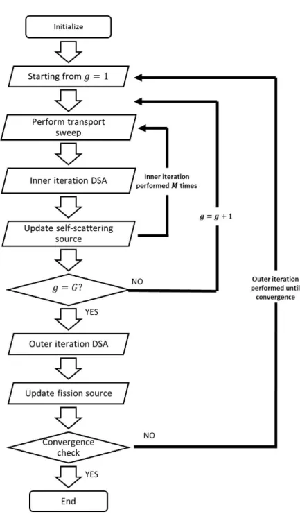
In the current work, the DSA method was investigated as a first attempt to accelerate the 2-energy-group neutron noise algorithm. The derivation and implementation of the DSA equations for the inner and outer iterations of the static module follow closely the work reported in [11] and [13]. The same approach is adapted to the acceleration of the inner and outer iterations of the dynamic module. The general DSA-based scheme is shown in Figure 3.3 and the details are discussed only for the dynamic calculations.

(25)

15

(26)

16

The dynamic module starts with the inner iterations, in which Eq. (3.13) is solved for

𝛿𝛿𝜓𝜓

��_𝑚𝑚(𝑙𝑙,m+1/2)_{and used to update the scalar neutron noise}_{𝛿𝛿𝜙𝜙}_��

𝑚𝑚(𝑙𝑙,𝑚𝑚+1/2) (instead of 𝛿𝛿𝜙𝜙��𝑚𝑚(𝑙𝑙,𝑚𝑚+1) in

the unaccelerated case) with the quadrature formula:

δ𝜙𝜙 ��_𝐼𝐼�𝑙𝑙_,_𝐽𝐽,𝑚𝑚+12�₍_𝑖𝑖_{) =}π 2� 𝑤𝑤𝑚𝑚𝛿𝛿𝜓𝜓��𝑚𝑚,𝐼𝐼,𝐽𝐽 �𝑙𝑙,_{𝑚𝑚+12�} (𝑖𝑖) 𝑁𝑁0 n=1 (3. 27) In these inner iterations, the estimates of the scalar neutron noise 𝛿𝛿𝜙𝜙��𝑚𝑚(𝑙𝑙,𝑚𝑚+1/2) are adjusted in

order to favor convergence. The acceleration step at the (𝑚𝑚+ 1)-th inner iteration, within the (𝑙𝑙+ 1)-th outer iteration, consists of a low-order diffusion problem that provides the quantities

𝛿𝛿𝜋𝜋_𝑔𝑔(_,𝑙𝑙_𝐼𝐼+1,𝑚𝑚+1_/₂)_,_𝐽𝐽+1_/₂ located at cell vertices for the correction of the neutron noise associated with the

𝑔𝑔-th energy-group, at cell center positions. The discretized equation for the correction quantities reads as: 2 ∆𝜕𝜕𝐼𝐼�∆𝜕𝜕𝐽𝐽𝐷𝐷𝑔𝑔,𝐼𝐼,𝐽𝐽+∆𝜕𝜕𝐽𝐽+1𝐷𝐷𝑔𝑔,𝐼𝐼,𝐽𝐽+1� �𝛿𝛿𝜋𝜋𝑔𝑔,𝐼𝐼+1/2,𝐽𝐽+1/2 (𝑙𝑙,𝑚𝑚+1) _{− 𝛿𝛿𝜋𝜋} 𝑔𝑔(,𝑙𝑙𝐼𝐼−1,𝑚𝑚+1/2,)𝐽𝐽+1/2� − 2 ∆𝜕𝜕𝐼𝐼+1�∆𝜕𝜕𝐽𝐽𝐷𝐷𝑔𝑔,𝐼𝐼+1,𝐽𝐽+∆𝜕𝜕𝐽𝐽+1𝐷𝐷𝑔𝑔,𝐼𝐼+1,𝐽𝐽+1� �𝛿𝛿𝜋𝜋𝑔𝑔,𝐼𝐼+3/2,𝐽𝐽+1/2 (𝑙𝑙,𝑚𝑚+1) _{− 𝛿𝛿𝜋𝜋} 𝑔𝑔(,𝑙𝑙𝐼𝐼+1,𝑚𝑚+1/2),𝐽𝐽+1/2� +_∆𝜕𝜕2 𝐽𝐽�∆𝜕𝜕𝐼𝐼𝐷𝐷𝑔𝑔,𝐼𝐼,𝐽𝐽+∆𝜕𝜕𝐼𝐼+1𝐷𝐷𝑔𝑔,𝐼𝐼+1,𝐽𝐽� �𝛿𝛿𝜋𝜋𝑔𝑔,𝐼𝐼+1/2,𝐽𝐽+1/2 (𝑙𝑙,𝑚𝑚+1) _{− 𝛿𝛿𝜋𝜋} 𝑔𝑔(,𝑙𝑙𝐼𝐼+1,𝑚𝑚+1/2),𝐽𝐽−1/2� − 2 ∆𝜕𝜕𝐽𝐽+1�∆𝜕𝜕𝐼𝐼𝐷𝐷𝑔𝑔,𝐼𝐼,𝐽𝐽+1+∆𝜕𝜕𝐼𝐼+1𝐷𝐷𝑔𝑔,𝐼𝐼+1,𝐽𝐽+1� �𝛿𝛿𝜋𝜋𝑔𝑔,𝐼𝐼+1/2,𝐽𝐽+3/2 (𝑙𝑙,𝑚𝑚+1) _{− 𝛿𝛿𝜋𝜋} 𝑔𝑔(,𝑙𝑙𝐼𝐼+1,𝑚𝑚+1/2),𝐽𝐽+1/2� +�� 𝛴𝛴𝑅𝑅,𝑔𝑔,𝐼𝐼′,𝐽𝐽′𝑉𝑉𝐼𝐼′,𝐽𝐽′� 𝐽𝐽+1 𝐽𝐽′_=𝐽𝐽 𝐼𝐼+1 𝐼𝐼′_=𝐼𝐼 � 𝛿𝛿𝜋𝜋_𝑔𝑔(_,𝑙𝑙_𝐼𝐼+1,𝑚𝑚+1_/₂)_,_𝐽𝐽+1_/₂=� � 𝛴𝛴𝑠𝑠𝑠𝑠,𝑔𝑔,𝐼𝐼′,𝐽𝐽′𝑉𝑉𝐼𝐼′,𝐽𝐽′�𝛿𝛿𝜙𝜙𝑔𝑔(𝑙𝑙,𝐼𝐼′,𝑚𝑚+1,𝐽𝐽′ /2)− 𝛿𝛿𝜙𝜙𝑔𝑔(𝑙𝑙,𝐼𝐼′,𝑚𝑚,𝐽𝐽′)� 𝐽𝐽+1 𝐽𝐽′_=𝐽𝐽 𝐼𝐼+1 𝐼𝐼′_=𝐼𝐼 (3. 28) where 𝐷𝐷𝑔𝑔,𝐼𝐼,𝐽𝐽 = 1 �3𝛴𝛴_𝑡𝑡𝑑𝑑𝑦𝑦𝑚𝑚_,_𝑔𝑔_,_𝐼𝐼_,_𝐽𝐽� (3. 29) 𝛴𝛴𝑅𝑅,𝑔𝑔,𝐼𝐼,𝐽𝐽 =𝛴𝛴𝑡𝑡𝑑𝑑𝑦𝑦𝑚𝑚,𝑔𝑔,𝐼𝐼,𝐽𝐽− 𝛴𝛴𝑠𝑠𝑠𝑠,𝑔𝑔,𝐼𝐼,𝐽𝐽 (3. 30)

Eq. (3.28) is a fixed source problem and by taking all the cell (𝐼𝐼, 𝐽𝐽) of the discretized domain, a system of linear equations is built for each energy group, and then it is solved with the LU factorization method. Instead of the update equation used in the unaccelerated scheme (Eq. 3.25) to calculate the scalar neutron noise for next inner iteration, the calculated quantities

𝛿𝛿𝜋𝜋_𝑔𝑔(_,𝑙𝑙_𝐼𝐼+1,𝑚𝑚+1_/₂)_,_𝐽𝐽+1_/₂ are used to modify cell center scalar neutron noise as follows:

𝛿𝛿𝜙𝜙_𝑔𝑔(𝑙𝑙_,_𝐼𝐼,𝑚𝑚+1_,_𝐽𝐽 ) =𝛿𝛿𝜙𝜙_𝑔𝑔�𝑙𝑙_,_𝐼𝐼,𝑚𝑚+12�_,_𝐽𝐽 +₄1� � 𝛿𝛿𝜋𝜋_𝑔𝑔(_,𝑙𝑙_𝐼𝐼,′𝑚𝑚+1₋₁_/₂)_,_𝐽𝐽′₋₁_/₂ 𝐽𝐽+1 𝐽𝐽′_=𝐽𝐽 𝐼𝐼+1 𝐼𝐼′_=𝐼𝐼 (3. 31) The new values given by Eq. (3.31) updates the self-scattering term in Eq. (3.13) before the next inner iteration. As in the unaccelerated case, 𝑀𝑀 inner iterations are performed for each energy group.

(27)

17

When the inner iterations are completed for all the energy groups, the calculation continues with the outer iteration. For the acceleration of the (𝑙𝑙+ 1)-th outer iteration, the correction quantities𝛿𝛿𝛿𝛿��_𝑔𝑔(_,𝑙𝑙+1_𝐼𝐼+1)_/₂_,_𝐽𝐽+1_/₂ for both energy groups are calculated at the cell vertices using the following equation: 2 ∆𝜕𝜕𝐼𝐼�∆𝜕𝜕𝐽𝐽𝐷𝐷�𝐼𝐼,𝐽𝐽+∆𝜕𝜕𝐽𝐽+1𝐷𝐷�𝐼𝐼,𝐽𝐽+1��𝛿𝛿𝛿𝛿 ��_𝐼𝐼+1(𝑙𝑙+1_/₂)_,_𝐽𝐽+1_/₂_{− 𝛿𝛿𝛿𝛿}_�� 𝐼𝐼−1(𝑙𝑙+1/2),𝐽𝐽+1/2� −_∆𝜕𝜕2 𝐼𝐼+1�∆𝜕𝜕𝐽𝐽𝐷𝐷�𝐼𝐼+1,𝐽𝐽+∆𝜕𝜕𝐽𝐽+1𝐷𝐷�𝐼𝐼+1,𝐽𝐽+1��𝛿𝛿𝛿𝛿��𝐼𝐼+3/2,𝐽𝐽+1/2 (𝑙𝑙+1) _{− 𝛿𝛿𝛿𝛿}_�� 𝐼𝐼+1(𝑙𝑙+1/2),𝐽𝐽+1/2� +_∆𝜕𝜕2 𝐽𝐽�∆𝜕𝜕𝐼𝐼𝐷𝐷�𝐼𝐼,𝐽𝐽+∆𝜕𝜕𝐼𝐼+1𝐷𝐷�𝐼𝐼+1,𝐽𝐽��𝛿𝛿𝛿𝛿 ��_𝐼𝐼+1(𝑙𝑙+1_/₂)_,_𝐽𝐽+1_/₂_{− 𝛿𝛿𝛿𝛿}_�� 𝐼𝐼+1(𝑙𝑙+1/2),𝐽𝐽−1/2� −_∆𝜕𝜕2 𝐽𝐽+1�∆𝜕𝜕𝐼𝐼𝐷𝐷�𝐼𝐼,𝐽𝐽+1+∆𝜕𝜕𝐼𝐼+1𝐷𝐷�𝐼𝐼+1,𝐽𝐽+1��𝛿𝛿𝛿𝛿��𝐼𝐼+1/2,𝐽𝐽+3/2 (𝑙𝑙+1) _{− 𝛿𝛿𝛿𝛿}_�� 𝐼𝐼+1(𝑙𝑙+1/2),𝐽𝐽+1/2� +�� 𝛴𝛴��𝑅𝑅_,_𝐼𝐼′_,_𝐽𝐽′𝑉𝑉𝐼𝐼′,𝐽𝐽′� 𝐽𝐽+1 𝐽𝐽′_=𝐽𝐽 𝐼𝐼+1 𝐼𝐼′_=𝐼𝐼 � 𝛿𝛿𝛿𝛿��_𝐼𝐼+1(𝑙𝑙+1_/₂)_,_𝐽𝐽+1_/₂ − �� 𝛴𝛴��𝑠𝑠𝑑𝑑_,_𝐼𝐼′_,_𝐽𝐽′𝑉𝑉𝐼𝐼′_,_𝐽𝐽′� 𝐽𝐽+1 𝐽𝐽′_=𝐽𝐽 𝐼𝐼+1 𝐼𝐼′_=𝐼𝐼 � 𝛿𝛿𝛿𝛿�� 𝐼𝐼+12,_𝐽𝐽+12 (𝑙𝑙+1) ₌_{� � χ�} I′_,_J′νΣ��_f_I′_,_J′𝑉𝑉_𝐼𝐼′_,_𝐽𝐽′�𝛿𝛿𝜙𝜙��_𝐼𝐼(′𝑙𝑙_,,_𝐽𝐽𝑀𝑀′)− 𝛿𝛿𝜙𝜙��_𝐼𝐼(′𝑙𝑙_,)_𝐽𝐽′� 𝐽𝐽+1 𝐽𝐽′_=𝐽𝐽 𝐼𝐼+1 𝐼𝐼′_=𝐼𝐼 (3. 32) with 𝛿𝛿𝛿𝛿 ��_𝐼𝐼+1(𝑙𝑙+1_/₂)_,_𝐽𝐽+1_/₂ ₌_�𝛿𝛿𝛿𝛿𝑔𝑔=1(𝑙𝑙+1,𝐼𝐼+1) /2,𝐽𝐽+1/2 𝛿𝛿𝛿𝛿_𝑔𝑔=2(𝑙𝑙+1_,_𝐼𝐼+1) _/₂_,_𝐽𝐽+1_/₂� (3. 33)

Eq. (3.32) also represents a fixed source problem where the two energy groups are coupled. Therefore, the linear system constructed for the overall discretized domain, in each outer iteration, includes both energy groups. The calculated values of 𝛿𝛿𝛿𝛿��_𝐼𝐼+1(𝑙𝑙+1_/₂)_,_𝐽𝐽+1_/₂ are used to correct the neutron noise at cell centers with the following relationship:

𝛿𝛿𝜙𝜙 ��_𝐼𝐼(_,𝑙𝑙+1_𝐽𝐽 ) ₌_{𝛿𝛿𝜙𝜙}_�� 𝐼𝐼(,𝑙𝑙𝐽𝐽,𝑀𝑀)+1₄� � 𝛿𝛿𝛿𝛿��𝐼𝐼(′𝑙𝑙+1₋₁_/)₂_,_𝐽𝐽′₋₁_/₂ 𝐽𝐽+1 𝐽𝐽′_=𝐽𝐽 𝐼𝐼+1 𝐼𝐼′_=𝐼𝐼 (3. 34) Before checking whether the calculation has converged, an updated evaluation of the fission source term of Eq. (3.13) is obtained from the new values of 𝛿𝛿𝜙𝜙��_𝐼𝐼(_,𝑙𝑙+1_𝐽𝐽 ). According to the outcome of the convergence criteria, the calculation is stopped or the next inner-outer iteration is started. As mentioned above, the accelerated iterative scheme applied in the static and dynamic modules are similar. However, the calculation of the static neutron fluxes requires the update of the value

of 𝑘𝑘𝑒𝑒𝑒𝑒𝑒𝑒 in the fission source term after every outer iteration, while the neutron noise is

(28)

(29)

Chapter 4 Verification of the neutron noise solver

19

Chapter 4 Verification of the neutron noise solver

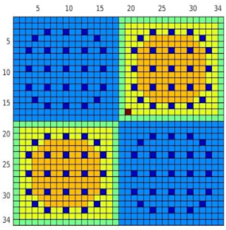
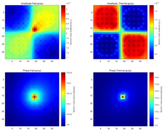
The performance of the dynamic module in the frequency domain is examined. In Section 4.1, the convergence rate of the unaccelerated and DSA inner-outer iteration schemes for dynamic calculations is studied in the case of an infinite homogeneous system. In Section 4.2, a neutron noise problem in a 2-D heterogeneous system was simulated with the SN solver and the results are compared with the ones obtained from the diffusion-based solver CORE SIM [4].

4.1 Fourier convergence analysis of the dynamic module

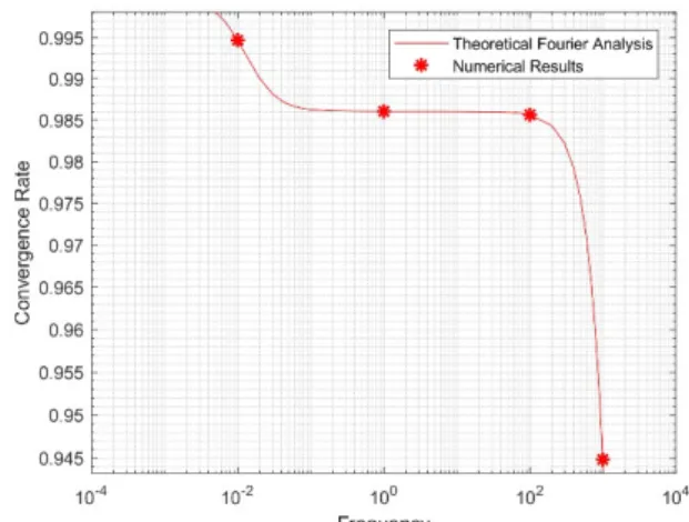
The Fourier convergence analysis method has been widely applied to deterministic neutron transport methods for static calculations [14] and to some extent for time-dependent calculations [15]. The convergence rate of the dynamic module is estimated from the analytical Fourier analysis and compared to numerical results generated by the SN solver.

In Paper I, the theoretical analysis is based on the one-dimensional continuous form of the iterative equations, while the numerical analysis is performed for a two-dimensional problem. In static calculations, it was shown in [16] that the theoretical results do not depend on the numbers of spatial dimensions when the diamond differencing method is considered. For the dynamic calculations, the same outcome is observed. The Fourier analysis reported below, is based on two-dimensional fully discretized equations.

4.1.1 Spectral radius for the unaccelerated scheme

The 2-dimensional system under study is homogeneous, so cross-sections and kinetic parameters are independent on the spatial position. The spatial discretization is such that the mesh nodes are identical with constant ∆𝜕𝜕 and ∆𝜕𝜕. The spatial vector that identifies the centre of the node (𝐼𝐼, 𝐽𝐽) is defined as:

𝑟𝑟⃗= ��𝐼𝐼 −1₂� ∆x,�𝐽𝐽 −1

2� ∆y�, 𝐼𝐼= 1, …𝐼𝐼𝑚𝑚𝑚𝑚𝑚𝑚,𝐽𝐽= 1, … ,𝐽𝐽𝑚𝑚𝑚𝑚𝑚𝑚 (4. 1) Additional spatial vectors to locate the surfaces and vertices of the nodes are defined as:

𝑎𝑎1

��⃗= �∆𝜕𝜕_{2 , 0}�, ��⃗𝑎𝑎2 =�0,∆𝜕𝜕₂ � (4. 2)

Using the notations above, the location of surface with index (𝐼𝐼+ 1/2,𝐽𝐽) can be given by 𝑟𝑟⃗+

𝑎𝑎1

��⃗. Similarly, the vertex location with index (𝐼𝐼+ 1/2,𝐽𝐽+ 1/2) can be expressed as 𝑟𝑟⃗+𝑎𝑎��⃗1+

𝑎𝑎2

(30)

20

The errors for the angular neutron noise (at the surfaces or at the center of a cell) and the scalar neutron noise are respectively:

𝛿𝛿𝜓𝜓 ��_𝑚𝑚err,(𝑙𝑙,𝑚𝑚+1/2) ₌_{𝛿𝛿𝜓𝜓}_�� 𝑚𝑚− 𝛿𝛿𝜓𝜓��𝑚𝑚(𝑙𝑙,𝑚𝑚+1/2) (4. 3) and δ𝜙𝜙 ��_𝐼𝐼𝑒𝑒𝑒𝑒𝑒𝑒_,_𝐽𝐽 ,(𝑙𝑙,𝑚𝑚) ₌ _δ𝜙𝜙_�� 𝐼𝐼,𝐽𝐽− δ𝜙𝜙��𝐼𝐼(,𝑙𝑙𝐽𝐽,𝑚𝑚) (4. 4)

where 𝛿𝛿𝜓𝜓��𝑚𝑚 and δ𝜙𝜙��𝐼𝐼,𝐽𝐽 are the exact (or converged) solutions and 𝛿𝛿𝜓𝜓��𝑚𝑚(𝑙𝑙,𝑚𝑚+1/2) and δ𝜙𝜙��𝐼𝐼(,𝑙𝑙𝐽𝐽,𝑚𝑚) are the

values estimated at the 𝑚𝑚-th inner iteration, within the (𝑙𝑙+ 1)-th outer iteration.

In the case of the unaccelerated scheme, the equation for the error quantities is obtained by subtracting Eq. (3.13) from Eq. (3.6):

𝜇𝜇𝑚𝑚 ∆𝜕𝜕 �𝛿𝛿𝜓𝜓��𝑚𝑚𝑒𝑒𝑒𝑒𝑒𝑒,𝐼𝐼+1,(𝑙𝑙/,𝑚𝑚+12,𝐽𝐽 /2)(𝑖𝑖)− 𝛿𝛿𝜓𝜓��𝑚𝑚𝑒𝑒𝑒𝑒𝑒𝑒,𝐼𝐼−1,(𝑙𝑙/,𝑚𝑚+12,𝐽𝐽 /2)(𝑖𝑖)�+ 𝜂𝜂𝑚𝑚 ∆𝜕𝜕 �𝛿𝛿𝜓𝜓��𝑚𝑚𝑒𝑒𝑒𝑒𝑒𝑒,𝐼𝐼,𝐽𝐽+1,(𝑙𝑙,𝑚𝑚+1/2 /2)(ω)− 𝛿𝛿𝜓𝜓��𝑚𝑚𝑒𝑒𝑒𝑒𝑒𝑒,𝐼𝐼,𝐽𝐽−1,(𝑙𝑙,𝑚𝑚+1/2 /2)(ω)� +��𝛴𝛴_tdyn_,_𝐼𝐼_,_𝐽𝐽 𝛿𝛿𝜓𝜓��_𝑚𝑚𝑒𝑒𝑒𝑒𝑒𝑒_,_𝐼𝐼_,_𝐽𝐽,(𝑙𝑙,𝑚𝑚+1/2)(𝑖𝑖) = 1 2π 𝛴𝛴��𝑠𝑠𝑠𝑠𝐼𝐼,𝐽𝐽δ𝜙𝜙��𝐼𝐼𝑒𝑒𝑒𝑒𝑒𝑒,𝐽𝐽 ,(𝑙𝑙,𝑚𝑚)(𝑖𝑖) +_{2π 𝛴𝛴}1 ��𝑠𝑠𝑑𝑑_𝐼𝐼_,_𝐽𝐽 δ𝜙𝜙��𝐼𝐼𝑒𝑒𝑒𝑒𝑒𝑒,𝐽𝐽 ,(𝑙𝑙,𝑀𝑀)(𝑖𝑖) +₂1_{𝜋𝜋 𝜒𝜒̿}𝐼𝐼,𝐽𝐽𝜈𝜈𝛴𝛴��𝑒𝑒_𝐼𝐼_,_𝐽𝐽δ𝜙𝜙��𝐼𝐼𝑒𝑒𝑒𝑒𝑒𝑒,𝐽𝐽 ,(𝑙𝑙,0)(𝑖𝑖) (4. 5)

Eq. (4.5) is similar to Eq. (3.13), but the angular and the scalar neutron noise are replaced by the corresponding error quantities and the source term is equal to zero. Then the rate of convergence for the solution of Eq. (3.13) is equivalent to the rate at which the error quantities tend to zero.

In order to study the rate at which the error quantities tend to zero, it is convenient to define the error quantities according to the following Fourier ansatz:

δ𝜙𝜙 ��_𝐼𝐼𝑒𝑒𝑒𝑒𝑒𝑒_,_𝐽𝐽 ,(𝑙𝑙)₍_𝑟𝑟⃗_,_𝑖𝑖_{) =}_𝐴𝐴̿₍_𝑙𝑙₎₍_𝑖𝑖₎_{𝑏𝑏�𝑒𝑒}_𝑚𝑚Θ_{��⃗∙𝑒𝑒⃗} _{(4. 6)} 𝛿𝛿𝜓𝜓 ��_𝑚𝑚err_,_𝐼𝐼_,_𝐽𝐽,(l,m+1/2)₍ 𝑟𝑟⃗,𝑖𝑖) =𝐴𝐴̿(𝑙𝑙)₍_𝑖𝑖₎_𝛼𝛼� 𝑚𝑚(𝑙𝑙,𝑚𝑚)(𝑖𝑖)𝑏𝑏�𝑒𝑒𝑚𝑚Θ��⃗∙𝑒𝑒⃗ (4. 7) 𝛿𝛿𝜓𝜓 ��_𝑚𝑚err_,_𝐼𝐼+1,(l,_/m+1₂_,_𝐽𝐽 /2)₍_𝑟𝑟⃗_,_𝑖𝑖_{) =}_𝐴𝐴̿(𝑙𝑙)₍_𝑖𝑖₎_𝛼𝛼� 𝑚𝑚(𝑙𝑙,𝑚𝑚)(𝑖𝑖)𝑏𝑏�𝑒𝑒𝑚𝑚Θ��⃗∙(𝑒𝑒⃗+𝑚𝑚��⃗1) (4. 8) 𝛿𝛿𝜓𝜓 ��_𝑚𝑚err_,_𝐼𝐼−1,(l,_/m+1₂_,_𝐽𝐽 /2)₍_𝑟𝑟⃗_,_𝑖𝑖_{) =}_𝐴𝐴̿₍_𝑙𝑙₎₍_𝑖𝑖₎_𝛼𝛼� 𝑚𝑚(𝑙𝑙,𝑚𝑚)(𝑖𝑖)𝑏𝑏�𝑒𝑒𝑚𝑚Θ��⃗∙(𝑒𝑒⃗−𝑚𝑚��⃗1) (4. 9) 𝛿𝛿𝜓𝜓 ��_𝑚𝑚err_,_𝐼𝐼_,_𝐽𝐽+1,(l,m+1_/₂ /2)₍_𝑟𝑟⃗_,_𝑖𝑖_{) =}_𝐴𝐴̿₍_𝑙𝑙₎₍_𝑖𝑖₎_𝛼𝛼� 𝑗𝑗(𝑙𝑙,𝑚𝑚)(𝑖𝑖)𝑏𝑏�𝑒𝑒𝑚𝑚Θ��⃗∙(𝑒𝑒⃗+𝑚𝑚��⃗2) (4. 10) 𝛿𝛿𝜓𝜓 ��_𝑚𝑚err_,_𝐼𝐼_,_𝐽𝐽−1,(l,m+1_/₂ /2)₍_𝑟𝑟⃗_,_𝑖𝑖_{) =}_𝐴𝐴̿₍_𝑙𝑙₎₍_𝑖𝑖₎_𝛼𝛼� 𝑗𝑗(𝑙𝑙,𝑚𝑚)(𝑖𝑖)𝑏𝑏�𝑒𝑒𝑚𝑚Θ��⃗∙(𝑒𝑒⃗−𝑚𝑚��⃗2) (4. 11) δ𝜙𝜙 ��_𝐼𝐼𝑒𝑒𝑒𝑒𝑒𝑒_,_𝐽𝐽 ,(𝑙𝑙,𝑚𝑚)₍_𝑟𝑟⃗_,_𝑖𝑖_{) =}_𝐴𝐴̿(𝑙𝑙)₍_𝑖𝑖₎_𝜉𝜉̿ 𝑢𝑢𝑚𝑚(𝑙𝑙,𝑚𝑚,2−𝐷𝐷) (𝑖𝑖)𝑏𝑏�𝑒𝑒𝑚𝑚Θ��⃗∙𝑒𝑒⃗ (4. 12)

In Eqs. (4.6) to (4.12), 𝛩𝛩�⃗ = (𝛩𝛩1,𝛩𝛩2) is the Fourier error mode. It consists of two components

that are, respectively, the error modes in the 𝜕𝜕 and 𝜕𝜕 directions and can take any values in the interval [−∞, +∞]. The elements of the column vector 𝑏𝑏� are equal to 1. The matrix 𝐴𝐴̿(𝑙𝑙)_is

diagonal and each element of the diagonal is associated with the error for one neutron energy group, after the 𝑙𝑙-th outer iteration. The matrices 𝛼𝛼�𝑚𝑚(𝑙𝑙,𝑚𝑚), 𝛼𝛼�𝑚𝑚(𝑙𝑙,𝑚𝑚), 𝛼𝛼�𝑗𝑗(𝑙𝑙,𝑚𝑚) and 𝜉𝜉̿𝑢𝑢𝑚𝑚(𝑙𝑙,𝑚𝑚,2−𝐷𝐷) are diagonal

(31)

21

matrices, and each element of the diagonal is associated with the error for one neutron energy group at the 𝑚𝑚-th inner iteration, within the (𝑙𝑙+ 1)-th outer iteration.

The convergence rate is related to the variation of the matrix 𝐴𝐴̿ between the two successive outer iterations 𝑙𝑙 and 𝑙𝑙+ 1. This variation depends on the properties of the matrix 𝜉𝜉̿_{𝑢𝑢𝑚𝑚}(𝑙𝑙,𝑚𝑚_,_2−𝐷𝐷) . In fact, once all the prescribed 𝑀𝑀 inner iterations are performed within the (𝑙𝑙+ 1)-th outer iteration, the error δ𝜙𝜙��_𝐼𝐼𝑒𝑒𝑒𝑒𝑒𝑒_,_𝐽𝐽 ,(𝑙𝑙,𝑀𝑀) given by Eq. (4.12) is equal to the error δ𝜙𝜙��_𝐼𝐼𝑒𝑒𝑒𝑒𝑒𝑒_,_𝐽𝐽 ,(𝑙𝑙+1) given by Eq. (4.6) at the end of the (𝑙𝑙+ 1)-th outer iteration, i.e.:

𝐴𝐴̿(𝑙𝑙+1) ₌_𝐴𝐴̿(𝑙𝑙)₍_𝑖𝑖₎_𝜉𝜉̿

𝑢𝑢𝑚𝑚(𝑙𝑙,𝑀𝑀,2−𝐷𝐷) (4. 13)

For the determination of 𝜉𝜉̿_{𝑢𝑢𝑚𝑚}(𝑙𝑙,𝑀𝑀_,_2−𝐷𝐷) , the Fourier ansatz is entered in Eq. (4.5) and 𝑒𝑒𝑚𝑚Θ��⃗∙𝑒𝑒⃗_is

eliminated from all the terms. The expressions:

𝑒𝑒𝑚𝑚Θ��⃗∙𝑚𝑚��⃗1− 𝑒𝑒−𝑚𝑚Θ��⃗∙𝑚𝑚��⃗1 = 2𝑤𝑤sin�𝛩𝛩₁Δ𝜕𝜕

2 � (4. 14)

𝑒𝑒𝑚𝑚Θ��⃗∙𝑚𝑚��⃗2 − 𝑒𝑒−𝑚𝑚Θ��⃗∙𝑚𝑚��⃗2 = 2𝑤𝑤sin�𝛩𝛩₂Δ𝜕𝜕

2� (4. 15)

are used in the first two terms of the left-hand side, so that the equation is rewritten as:

𝜇𝜇𝑚𝑚

∆𝜕𝜕 𝛼𝛼�𝑚𝑚(𝑙𝑙,𝑚𝑚)2𝑤𝑤sin�𝛩𝛩1Δ𝜕𝜕₂ �+_{∆𝜕𝜕 𝛼𝛼�}𝜂𝜂𝑚𝑚 𝑗𝑗(𝑙𝑙,𝑚𝑚)2𝑤𝑤sin�𝛩𝛩2Δ𝜕𝜕₂ �+𝛴𝛴��𝛼𝛼�𝑡𝑡𝑑𝑑𝑦𝑦𝑚𝑚 𝑚𝑚(𝑙𝑙,𝑚𝑚)

=_{2π 𝛴𝛴}1 ��𝜉𝜉̿𝑠𝑠𝑠𝑠 𝑢𝑢𝑚𝑚(𝑙𝑙,𝑚𝑚,2−𝐷𝐷) +_{2π 𝛴𝛴}1 ��𝑠𝑠𝑑𝑑 𝜉𝜉̿𝑢𝑢𝑚𝑚(𝑙𝑙,𝑀𝑀,2−𝐷𝐷) +_{2π χ�}1 νΣ��f (4. 16)

The coefficient matrices 𝛼𝛼�_𝑚𝑚(𝑙𝑙,𝑚𝑚) and 𝛼𝛼�_𝑗𝑗(𝑙𝑙,𝑚𝑚) are replaced with 𝛼𝛼�𝑚𝑚(𝑙𝑙,𝑚𝑚) through the relationships

derived from the diamond difference scheme:

𝛼𝛼�𝑚𝑚(𝑙𝑙,𝑚𝑚) = 1₂𝛼𝛼�𝑚𝑚(𝑙𝑙,𝑚𝑚)�𝑒𝑒𝑚𝑚𝛩𝛩��⃗∙𝑚𝑚��⃗1 +𝑒𝑒−𝑚𝑚𝛩𝛩��⃗∙𝑚𝑚��⃗1�=𝛼𝛼�𝑚𝑚(𝑙𝑙,𝑚𝑚)cos�𝛩𝛩1Δ𝜕𝜕₂ � (4. 17)

𝛼𝛼�𝑚𝑚(𝑙𝑙,𝑚𝑚) =1₂𝛼𝛼�𝑗𝑗(𝑙𝑙,𝑚𝑚)�𝑒𝑒𝑚𝑚𝛩𝛩��⃗∙𝑚𝑚��⃗2+𝑒𝑒−𝑚𝑚𝛩𝛩��⃗∙𝑚𝑚��⃗2�= 𝛼𝛼�𝑗𝑗(𝑙𝑙,𝑚𝑚)cos�𝛩𝛩2Δ𝜕𝜕₂� (4. 18)

As a result, Eq. (4.16) becomes:

𝜇𝜇𝑚𝑚 ∆𝜕𝜕 𝛼𝛼�𝑚𝑚(𝑙𝑙,𝑚𝑚)2𝑤𝑤tan�𝛩𝛩1 Δ𝜕𝜕 2�+ 𝜂𝜂𝑚𝑚 ∆𝜕𝜕 𝛼𝛼�𝑚𝑚(𝑙𝑙,𝑚𝑚)2𝑤𝑤tan�𝛩𝛩2 Δ𝜕𝜕 2 �+𝛴𝛴��𝛼𝛼�𝑡𝑡𝑑𝑑𝑦𝑦𝑚𝑚 𝑚𝑚(𝑙𝑙,𝑚𝑚) = 1 2π 𝛴𝛴��𝜉𝜉̿𝑠𝑠𝑠𝑠 𝑢𝑢𝑚𝑚(𝑙𝑙,𝑚𝑚,2−𝐷𝐷) + 1 2π 𝛴𝛴��𝑠𝑠𝑑𝑑 𝜉𝜉̿𝑢𝑢𝑚𝑚(𝑙𝑙,𝑀𝑀,2−𝐷𝐷) + 1 2π χ�νΣ��f (4. 19)

Isolating 𝛼𝛼�𝑚𝑚(𝑙𝑙,𝑚𝑚) leads to:

𝛼𝛼�𝑚𝑚(𝑙𝑙,𝑚𝑚) = _{2π ∙}1 𝛴𝛴��𝜉𝜉̿𝑠𝑠𝑠𝑠 𝑢𝑢𝑚𝑚,2−𝐷𝐷 (𝑙𝑙,𝑚𝑚) ₊_𝛴𝛴 𝑠𝑠𝑑𝑑 ��_𝜉𝜉̿_{𝑢𝑢𝑚𝑚}(𝑙𝑙,𝑀𝑀_,_2−𝐷𝐷) ₊_χ�_νΣ f �� μn ∆x 2𝑤𝑤tan�Θ1Δ𝜕𝜕₂ �+η_∆n_{y 2}𝑤𝑤tan�Θ2Δ𝜕𝜕₂ �+𝛴𝛴��𝑡𝑡𝑑𝑑𝑦𝑦𝑚𝑚 (4. 20)