Issues in Design of Maximum-Power-Point-Tracking Control – Power Electronics Perspective

Issues in Design of Maximum-Power-Point-Tracking

Control

–

Power Electronics Perspective

Tampereen teknillinen yliopisto. Julkaisu 1571 Tampere University of Technology. Publication 1571

Jyri Kivimäki

Issues in Design of Maximum-Power-Point-Tracking

Control – Power Electronics Perspective

Thesis for the degree of Doctor of Science in Technology to be presented with due permission for public examination and criticism in Rakennustalo Building, Auditorium RG202, at Tampere University of Technology, on the 5th _{of October 2018, at 12 noon.}

Tampereen teknillinen yliopisto - Tampere University of Technology Tampere 2018

Doctoral candidate: Jyri Kivimäki

Laboratory of Electrical Energy Engineering Faculty of Computing and Electrical Engineering Tampere University of Technology

Finland

Supervisor: Teuvo Suntio, Professor

Laboratory of Electrical Energy Engineering Faculty of Computing and Electrical Engineering Tampere University of Technology

Finland

Pre-examiners: Giovanni Spagnuolo, Professor

Department of Information Engineering,

Electrical Engineering, and Applied Mathematics University of Salerno

Italy

Pertti Silventoinen, Professor School of Energy Systems

Lappeenranta University of Technology Finland

Opponents: Jorma Kyyrä, Professor

Department of Electrical Engineering and Automation Aalto University

Finland

Giovanni Spagnuolo, Professor

Department of Information Engineering,

Electrical Engineering, and Applied Mathematics University of Salerno

Italy

ISBN 978-952-15-4194-0 (printed) ISBN 978-952-15-4213-8 (PDF)

This thesis provides a comprehensive study of the dynamic characteristics and operation of maximum-power-point-tracking (MPPT) dc-dc converters, especially for those parts that concern the MPPT-control design. The study concentrates on the widely-utilized heuristic perturb-based MPPT algorithms and their design constraints when equipped with photovoltaic-interfacing converter. The main objective is to provide an explicit formulation of the input-power dynamics of the photovoltaic-generator-interfacing dc-dc converter for addressing the MPP-tracking control. The dynamics introduce design constraints for the aforementioned MPPT-control algorithms and provide tools for de-terministic MPPT design.

A photovoltaic (PV) generator has nonlinear current-voltage characteristics with a par-ticular maximum power point (MPP), which depends on the environmental factors such as temperature and irradiation. Thus, to ensure the maximization of the power extracted from the PV source, the interfacing power converter must be capable of controlling its parameters, i.e., changing its input voltage and current levels based on the MPP of the PV generator. That is done by implementing an MPPT controller, which generates the reference control signal for the interfacing converter. Despite the way of implementation, the fundamental operation is to find the electrical operating point, i.e., the voltage and the current, at which the PV generator either generates the maximum power or follows a given power reference at every time instant. However, the dynamic characteristics of a photovoltaic generator are determined by the environmental conditions as well as the dynamics of the interfacing converter, which creates limitations for the MPPT-control design. It has been noticed recently that the characteristic curve of a PV generator can be separated into three different operation regions each having their distinct char-acteristics. Thus, to ensure reliability and efficiency of a maximum-power tracking, all of these regions should be analyzed separately and choose the condition corresponding to the slowest settling dynamics of the PV system. Up to now, that is not completely recognized, and deterministic analytical models are missing to provide design guidelines for the MPPT-control design.

This thesis presents a detailed dynamic model for PV-generator power dynamics in case of open-loop and closed-loop-operated switched-mode dc-dc converter. Two common design examples of closed-loop-operated converters were provided, where the closed-loop dynamics of the converter was slow and fast by adjusting the control bandwidth and phase margin of the feedback loop. With the developed models, a proper evaluation of the MPPT control imposed by the converter dynamics was presented. Thus, previously developed design guidelines were revised, or new guidelines were established.

This research was carried out at the Laboratory of Electrical Energy Engineering (LEEE) at Tampere University of Technology (TUT) during the years 2015–2018. The research was mainly funded by TUT and ABB Ltd. In addition, the financial support received from Fortum Foundation is greatly appreciated.

First of all, I want to express my gratitude to Professor Teuvo Suntio for supervising my thesis and providing guidance throughout my journey towards the doctoral degree. Also, many discussions with Professor Seppo Valkealahti are highly valued. Secondly, I want to thank all my current and former colleagues who have influenced my research, especially D.Sc. (Tech.) Aapo Aapro, Assistant Professor Tuomas Messo, D.Sc. (Tech.) Jukka Viinam¨aki, D.Sc. (Tech.) Juha Jokipii, D.Sc. (Tech.) Jenni Rekola, D.Sc. (Tech.) Kari Lappalainen, M.Sc. Julius Schnabel, M.Sc. Matti Marjanen, M.Sc. Markku J¨arvel¨a, M.Sc. Matias Berg, B.Sc. Antti Hild´en and M.Sc. Roosa-Maria Sallinen for sharing your ideas and offering valuable comments during these years. It has been motivating to work together with highly talented people working with positive and encouraging attitude. Furthermore, all the staff at LEEE deserve my thanks for making these years at the university extremely pleasant by providing the great working environment. I am also most grateful to Professors Giovanni Spagnuolo and Pertti Silventoinen for examining my thesis and for the resulting supportive discussion which helped me to improve the quality of the thesis.

Finally, and most importantly, I want to thank my fianc´ee Nette, parents Marjatta and Reijo, and brother Antti for all the support and encouragement they have given me during my academic career.

Tampere, September 6, 2018

Abstract . . . iii

Preface . . . v

Contents . . . vi

Symbols and Abbreviations . . . ix

1. Introduction . . . 1

1.1 Electricity production using renewable energy sources . . . 1

1.2 Properties of a photovoltaic generator . . . 2

1.3 DC-DC converters in photovoltaic systems . . . 8

1.4 Maximum-power-point tracking in photovoltaic applications . . . 12

1.4.1 Overview of existing methods . . . 13

1.4.2 Reliability and efficiency of maximum-power-point tracking . . . 15

1.5 Objectives and scientific contributions . . . 22

1.6 Related publications and author’s contribution . . . 23

1.7 Structure of the thesis . . . 24

2. Modeling . . . 25

2.1 Photovoltaic generator . . . 25

2.2 Dynamic modeling of dc-dc converters . . . 30

2.2.1 State-space averaging . . . 30

2.2.2 Transient characteristics of first-order and second-order systems . . . . 33

2.2.3 Dynamic modeling under feedback control . . . 36

2.2.4 Effect of photovoltaic generator . . . 45

2.2.5 Dynamic model of a PVG-interfacing voltage-boosting dc-dc converter 47 2.3 Conclusions . . . 50

3. Maximum-power-point tracking in photovoltaic applications . . . 51

3.1 Perturbative MPPT techniques . . . 51

3.2 Perturbation frequency constraints . . . 54

3.2.1 Open-loop-operated converters . . . 55

3.2.2 Closed-loop-operated converters . . . 61

3.3 Perturbation step-size constraints . . . 66

3.3.1 Varying irradiance conditions . . . 69

3.3.2 The effect of different noise sources . . . 72

3.3.3 The effect of discontinuous inductor current . . . 74

4.1 Experimental setup . . . 81

4.2 Open-loop settling time estimation . . . 82

4.3 Closed-loop settling-time estimation . . . 84

4.3.1 I-type control . . . 84

4.3.2 PID-type control . . . 86

4.4 Maximum perturbation-step size based on discontinuous inductor current . 87 5. Conclusions . . . 91

5.1 Final conclusions . . . 91

5.2 Future research topics . . . 93

References . . . 95

A.Tables . . . 105

GREEK CHARACTERS

∆ Relative magnitude of settling time band, determinant

η Diode ideality factor

ηmppt Maximum-power-point-tracking efficiency L Laplace operator

ωd Damped natural angular frequency

ωn Undamped natural angular frequency of a open-loop-operated converter

ωn-c Undamped natural angular frequency of a closed-loop-operated converter ωp Input voltage controller pole angular frequency

ωs Grid fundamental angular frequency

ωz Input voltage controller zero angular frequency

ωz-esr Capacitor-induced zero angular frequency

ζ Damping factor

θ Phase angle

τ Time constant

LATIN CHARACTERS

A System coefficient matrix of the state-space representation

B Input coefficient matrix of the state-space representation

B Maximum bits in an analog-to-digital converter

C Output coefficient matrix of the state-space representation

cd Capacitance of a PV cell Cdc DC-link capacitance

C1 Capacitance of the input terminal capacitor C2 Capacitance of the output terminal capacitor

D, d Duty ratio

D0, d0 Complement of the duty ratio ∆D Increment in the duty ratio

D Input-output coefficient matrix of the state-space representation

fs Switching frequency

G Matrix containing transfer functions of a converter

G Irradiance

Gci Control-to-input transfer function

GcL Control-to-inductor current transfer function

Gco Control-to-output transfer function

Gio Input-to-output transfer function

Gise Input-current sensing gain Gv

se Input-voltage sensing gain

I Identity matrix of the state-space representation

H Auxiliary variable

Impp Current of the maximum-power point

ipv, Ipv Current of a photovoltaic generator

∆IG Incremental change in current due to variation in irradiance ∆Ix Incremental change in current due to perturbation step

∆Ipv Incremental change in the terminal current of a photovoltaic generator

id Diode current

iin Input current of a converter

iinS Input current of non-ideal source iL Inductor current

io Output current of a converter iph Photocurrent

ipv Terminal current of a photovoltaic generator k Boltzmann constant or time instant

Kc Input voltage controller gain Kph Material constant

L Inductance

Lin Input-voltage-control loop

N Scaling factor

Ns Number of series-connected cells in photovoltaic module

Np Number of parallel-connected cells in photovoltaic module

Ppv Average output power of a photovoltaic generator

∆PG Power change in a photovoltaic generator due to irradiance variation ∆Ppv Incremental change in the terminal power of a photovoltaic generator ∆Px Power change in a photovoltaic generator due to perturbation step

q Elementary charge

Rmpp Static resistance of a photovoltaic generator at maximum power point

Rpv Static resistance of a photovoltaic generator rC Equivalent resistance of an capacitor

rpv Dynamic resistance of a photovoltaic generator

rs Parasitic series resistance of a photovoltaic cell

rsh Parasitic shunt resistance of a photovoltaic cell

s Laplace variable

t, T Time

TK Temperature

Ts Switching period

Toi Reverse transfer function

T∆ Power settling time of a photovoltaic generator

u,U Vector containing Laplace transformed input variables

vadc Voltage resolution

Vd Diode threshold voltage Vdc DC-link voltage

Ve Low-frequency gain of a transfer function Vmpp Voltage of the maximum power point

vpv, Vpv Voltage of a photovoltaic generator

Vfs Full-scale voltage in analog-to-digital converter ∆Vo Amplitude of output voltage fluctuation

∆Vpv Incremental change in the terminal voltage of a photovoltaic generator ∆Vx Incremental change in voltage due to perturbation step

∆T Perturbation period of a maximum-power-point tracking algorithm

Vpv Terminal voltage of a photovoltaic generator

∆Vref

in Incremental change in input-voltage reference

x,X Vector containing Laplace transformed state variables ˆ

x AC-perturbation around a steady-state operation point

hxi Average value of variable x

∆x Incremental change in a perturbed variable

y Output variable, optimization function

y,Y Vector containing Laplace transformed output variables

Yo Output admittance

YS Output admittance of a non-ideal source

ac Alternating current ADC Analog-to-digital converter CC Constant current

CCM Continuous conduction mode CCR Constant-current region CPR Constant-power region CVR Constant-voltage region CF Current fed CV Constant voltage dc Direct current

DCM Discontinuous conduction mode

DMPPT Distributed maximum-power-point tracking ES Extremum seeking

ESR Equivalent series resistance GM Gain margin

IC Incremental conductance LSB Least significant bit MPP Maximum-power point

MPPT Maximum-power-point tracking OC Open circuit

PID Proportional integral derivative PM Phase margin

PV Photovoltaic

PVG Photovoltaic generator PWM Pulse width modulation P&O Perturb and observe RCC Ripple correlation control SC Short circuit

-c Refers to closed-loop transfer function in Refers to input-side transfer function max Refers to defined maximum value min Refers to defined minimum value

mpp, MPP Refers to operation at the maximum-power point -o Refers to open-loop transfer function

oc, OC Refers to operation in open-circuit condition -oco Refers to output terminal open-circuit out Refers to output-side transfer function

pv Refers to PV-generator affected function or variable p-p Refers to peak-to-peak value

sc, SC Refers to operation in short-circuit condition -sci Refers to input terminal short-circuit -∞ Refers to ideal transfer function

SUPERSCRIPTS

-1 Inverse operator

CCR Refers to operation in constant-current region CPR Refers to operation in constant-power region CVR Refers to operation in constant-voltage region I Refers to integral-controller-transfer function PID Refers to integral-controller-transfer function pv Refers to PV-generator affected function or variable -RO Refers to reduced-order transfer function

S Refers to source-affected transfer function T Transpose

This chapter introduces the background of the research, clarifies the motivation for the conducted research, and reviews the existing knowledge related to the topic.

1.1

Electricity production using renewable energy sources

Modern society has become increasingly dependent on energy. Since theIndustrial Rev-olution in the late 18th century, humankind has developed alternative ways to utilize energy for power generation and electrification purposes, which have accelerated depen-dency of energy. Up to now, coal with its different forms has been the primary source of energy. However, excessive use of these fossil fuels increases the emissions of carbon diox-ide, which have been shown to be the main contributor to the global warming. As shown in Table 1.1, fossil fuels are still dominating the world electricity generation. Thus, growing energy demand and the impact of the extensive use of fossil fuels has driven researchers to further develop renewable energy resources such as hydro, geothermal, biofuel, wind, and solar due to their lack of harmful emissions and being inexhaustible as primary energy sources [1]. As Table 1.1 indicates, hydro has already widely utilized and therefore, a significant increase is difficult to obtain. Thus, the highest potential of future electricity generation can be seen in other renewable energy sources.

Table 1.1: World electricity generation by source in 2015 [2].

Source Coal Natural gas Hydro Nuclear Renewables (excl. hydro) Oil Share (%) 39.3 22.9 16 10.6 7.1 4.1

Among renewable energy sources, solar energy seems to be the most appealing al-ternative to fossil fuels, because it is free, clean and abundantly available [3]. Energy from the Sun is carried by electromagnetic radiation, which can be measured to be 1361 W/m2 _{on the Earth’s upper atmosphere [4]. A significant amount of incoming radiation}

is either reflected or absorbed in the atmosphere, and therefore, average irradiance on the Earth’s surface can be measured to be around 1000 W/m2. Thus, the total solar power on the surface of the Earth can be approximated to be 86 PW [5]. According to [2], world energy consumption was approximated to be 109.1 PWh in 2015, which means that the solar power can fulfill the energy demand less than one and half hour. That

energy flow can be exploited to heat water by using a solar thermal collector, or it can be converted directly into electricity by using a photovoltaic (PV) generator.

Since the beginning of PV productization, solar energy has two main disadvantages: high costs and its unpredictability. The high price of the PV system is related to their low conversion efficiency, which has prevented the extensive adaption of solar energy. Research era of modern silicon-based PV cells for energy production can be considered to be started in 1954 when a PV cell with 6 % efficiency was developed [6]. Up to now, widely utilized wafer-based crystalline silicon modules have commercial efficiencies between 14 and 24 % [7]. In recent years, the combination of increased efficiency with reduced manufacturing costs, photovoltaic energy is approaching and has already reached in some countries, so-calledgrid parity, i.e., costs becomes equal or less than the electricity generated by utilizing the conventional energy sources such as fossil fuels.

As a consequence of the price development and political decisions, the installed solar photovoltaic capacity has increased significantly in recent years. Based on the latest published reports by International Energy Agency (IEA), global cumulative PV instal-lations continued its exponential growth reaching 303 GW by the end of 2016 indicating 50 % increase from the previous year [7] mainly due to the significant investments in the United States and Asia Pacific. Especially China and Japan, have a major contribution to the growth having over 30 % of the global cumulative PV capacity by the end of 2016. Along with the PV power price development, PV is becoming cost competitive with fossil fuels and onshore wind power [8]. Thus, the future challenges of photovoltaic can be seen to be its uncontrollability. Photovoltaic energy has strong daily and seasonal patterns, which in turn, also has a significant variance between successive years. Up to now, the energy demand characteristics of the consumers and the availability of the solar energy do not match with each other. Therefore, the standalone PV energy systems are not feasible as such. As a consequence, the way to fully exploiting the renewable energy is the grid connection, generally at the distribution level. An adaptation of various fast varying renewable sources requires intelligently controlled power electronic converter to fulfill the requirements of the grid connections, including frequency, voltage, control of active and reactive power and harmonic minimization, for example [9].

1.2

Properties of a photovoltaic generator

The operation of PV cells is based on the photovoltaic effect, which was first observed by Alexandre-Edmond Becquerel in 1839 and later explained by Albert Einstein in 1905. The fundamental behavior of photovoltaic phenomenon inside the p-n junction can be summarized as the absorption of solar irradiation, the generation and transport of free carriers and collection of these electric charges at the terminals of the cell. Essentially, a basic building block of every photovoltaic system is a single PV cell, where the generated

dc current in the p-n junction is determined by the area of the cell and the amount of exposed solar irradiation. PV cells can be classified as either wafer-based crystalline, compound semiconductor, or organic. Currently, crystalline silicon technologies (sin-gle crystal and multicrystalline silicon) account for more than 90 % of the overall cell production [7].

The terminal voltage of a single cell is in the order of 0.5 V. Thus several cells need to be connected in series to form panels (also known as modules) to fulfill the voltage and power requirements of a downstream system. Commercial PV panels contain typically 30 to 60 cells connected in series, yielding panel open-circuit voltage of approximately 20– 40 V with maximum-power-point (MPP) voltage of 18–32 V, and reaching power rating from 40 W to 400 W. The amount of maximum current can be increased by increasing the cell area or by connecting cells in parallel. PV panels can be further connected in series or parallel to form a PV array to increase voltage or current output, respectively. In general, the combination of interconnected PV subsystems is called PV generator (PVG) having the same fundamental characteristics as a single cell [10].

In order to model the effect of PVG on the interconnected system, a static electrical model is required. Several PV cell models have been introduced in literature differing in complexity and implementation purposes, where two main PV models proposed are the double-diode and the single-diode models [11]. Despite the higher accuracy of the double-diode model, it is not widely adopted due to parametrization difficulty and a high computational burden [12]. Thus, a single-diode model represented in [13] and shown in Fig. 1.1, is commonly used to model the static electrical characteristics of PV cell due to the excellent compromise between accuracy and complexity. Such a simplified electrical equivalent circuit of a PV cell composes of a photocurrent source with a parallel-connected diode and parasitic elements, where a non-ideal diode represents the internal semiconductor junction, and parasitic resistances correspond to the power losses.

An equation for PVG terminal current ipv can be formed based on non-closed-form Shockley diode equation as follows

ipv=NpIph−NpIs exp

vpv+Ns Nprsipv NsηkTK/q ! −1 ! − vpv+ Ns Nprsipvvpv Ns Nprsh , (1.1)

where Ns denotes the number of series-connected cells and Np the number of parallel-connected strings,Iphis the current generated by the incident light,Isis the diode reverse saturation current,q is the elementary charge,TK is the absolute temperature,k is the Boltzmann constant, andη is the diode ideality factor. Clearly, due to the non-closed-formed equation, numerical computational methods need to be used to calculate PV current in respect to PV voltage. It is worth noting that the accuracy of the PV model does not solely depend on its complexity but also the identification of equivalent circuit parameters. All the parameters may be extracted by utilizing manufacturer’s datasheet data [11, 14–16]. The datasheet generally gives information on the characteristics and performance in respect to the so-calledstandard test condition (STC), which corresponds to irradiation of 1000 W/m2 at 25◦C. Typically, only the values of open-circuit (OC) voltage, short-circuit (SC) current, MPP voltage and MPP current are provided, and therefore, the other parameters need to be derived.

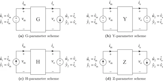
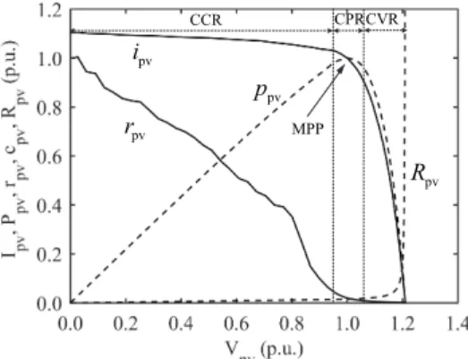
The PV cell can be considered to be a highly non-linear current source, which has lim-ited output voltage and power as well as distinct operation regions. The current-voltage (I-V) curve of a PV generator (cf. Fig. 1.2) contains two distinct regions separated by the MPP, which is created by the behavior of the diodes when they start conducting cur-rent along the increase in the cell terminal voltage. The operation regions are commonly categorized based on the variable, which stays practically constant within the named re-gion. Thus, constant current region (CCR) lies at the voltage less than the MPP voltage and constant voltage region (CVR) at the voltage higher than MPP voltage. The lower boundary of CCR and the upper boundary of CVR are limited by SC and OC conditions, respectively. A PV panel operates at SC if the PV-panel voltage Vpv is zero and at OC if the PV-panel current Ipv is zero, and therefore, the PV panel does not generate any power in either of these conditions. In addition to CCR and CVR, the third region can be determined around the MPP as shown in Fig. 1.2. That is because the finite resolution of the digitally controlled measurement system will make it impossible to locate exactly the MPP, and therefore, the vicinity of MPP will form a region, which can be named as the constant-power region (CPR), as explicitly justified in Section 2.1.

Figure 1.2 also illustrates the behavior of dynamic (rpv =−∆vpv/∆ipv) and static (Rpv=Vpv/Ipv) resistances of the PV panel. The dynamic resistance represents the

Fig. 1.2: Normalized behavior ofIpv,Vpv,Ppv,rpvandRpvwhen the operating point is varied.

that the current is flowing out form the PVG. As shown in the figure, the dynamic resistance is non-linear and operation-point dependent. Dynamic resistance is higher than the static resistance in CCR, whereas the relation is opposite in CVR. At the MPP, the derivative of PVG output powerppvis zero, which can be represented by (1.2). Thus, static and dynamic resistances are equal at MPP as stated in [17].

dppv dvpv = d(vpvipv) dvpv =Vpv+Ipv ∆vpv ∆ipv = 0 ⇔ Vpv Ipv =− ∆vpv ∆ipv, (1.2)

Photovoltaic cells are highly affected by operating conditions. These are mainly the value of irradiance on a PV cell and the temperature of the p-n junction. In Fig. 1.3, two power-voltage (P-V) curves were plotted based on (1.1) with different irradiance and temperature levels scaled to per unit values for convenience. As illustrated in Fig. 1.3a, the PV-generated current is directly proportional to incoming irradiation. Thus, the maximum power can be achieved in bright sunshine conditions. The maximum power can be extracted while the PVG is operated at MPP voltage, which stays practically constant along different irradiance levels. As the figure indicates, however, the irradiance also affects slightly the OC voltage shifting the MPP voltage correspondingly. The effect is much smaller than the effect of the irradiance, and it is only noticeable at very low irradiance levels, which in turn, are not reached in practical applications due to the existing diffuse irradiance. In contrast, as can be seen in Fig. 1.3b, the temperature of a PV cell has a significant effect on the OC voltage also affecting the MPP voltage. The silicon has a negative temperature coefficient, approximately -2.3 mV/◦C, hence the maximum power is achieved at low temperature and bright sunshine conditions. In the Northern hemisphere, for instance, that means that maximum PVG power peaks can be expected in spring at the beginning of the second quarter of the year.

0 0.2 0.4 0.6 0.8 1 1.2 Voltage (p.u.) 0 0.2 0.4 0.6 0.8 1 1.2 Power (p.u.)

(a) The effect of irradiance

0 0.2 0.4 0.6 0.8 1 1.2 Voltage (p.u.) 0 0.2 0.4 0.6 0.8 1 1.2 Power (p.u.)

(b)The effect of temperature Fig. 1.3: The effect of temperature and irradiance on P-V curve of a PV panel.

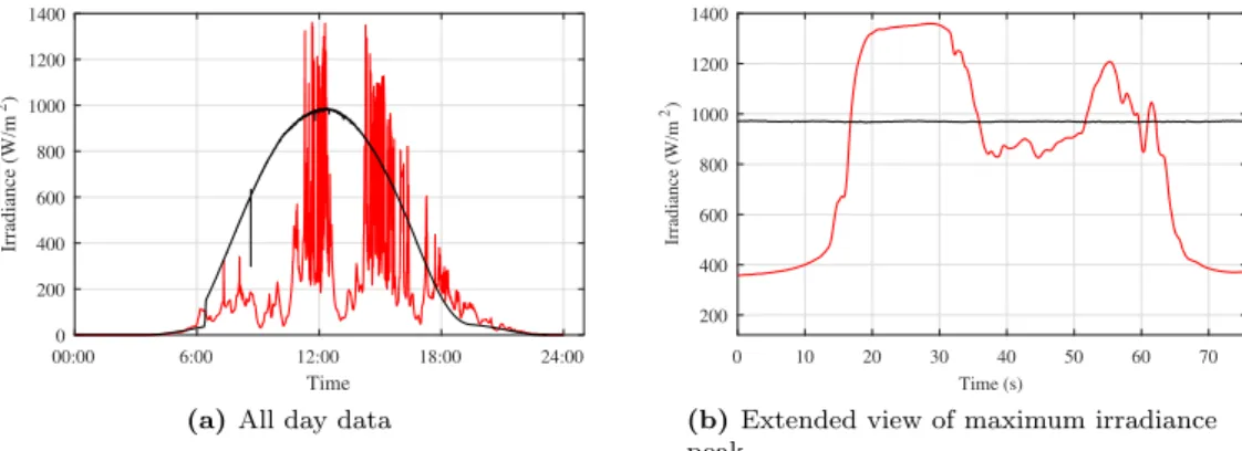
PV systems are prone to irradiance fluctuations caused by overpassing cloud shadows that are the main cause of fluctuating PV power production. Since the MPP voltage stays practically constant along the day, the output power of the PV system is directly proportional to the highly-varying irradiance-dependent PV current. The unpredictable behavior of the PV system is illustrated in Fig. 1.4 showing the behavior of irradiance curves during two particular days recorded on the rooftop of Tampere University of Tech-nology. The black line represents the typical clear sky day yielding uniform parabolic irradiance distribution along the day while the irradiance is typically maximized at noon. The nominal value of the direct and diffused irradiations at the Earth’s surface is consid-ered to be 1000 W/m2, but it is naturally varied depending on the atmospheric conditions and the angle of incidence of the irradiation over the location of the PV panel.

In contrast, the red line represents the half-cloudy day when the clouds are moving over the PV panels removing the direct irradiation temporarily from the spectrum of the light on the surface of the PV panels. In that case, several decreased and increased irradiance variations occur during the day indicating the problematic behavior of the varying irradiance conditions. According to [18–20], the usual and maximum irradiance slopes are considered to be 30 or 100 W/m2_{s, while the maximum value for irradiance is}

considered to be STC irradiance, i.e., 1000 W/m2_{, which are further utilized for designing}

MPP-tracking control, for instance. However, as shown in Fig. 1.4, these values can be exceeded due to fast-moving passing-by clouds yielding potential problems in PV systems if they are not taken into account. As the PV power production replaces more traditional non-weather-dependent power sources, power fluctuating PV systems need to be supported by other forms of electricity productions. Therefore, it is clear that PV systems increase technical requirements for the interconnected systems in order to control

the grid power according to the grid requirements [21]. 00:00 6:00 12:00 18:00 24:00 Time 0 200 400 600 800 1000 1200 1400 Irradiance (W/m 2)

(a) All day data

0 10 20 30 40 50 60 70 Time (s) 200 400 600 800 1000 1200 1400 Irradiance (W/m 2)

(b)Extended view of maximum irradiance peak

Fig. 1.4: The behavior of irradiance during particular clear-sky (black line) and half-cloudy (red line) day.

In addition to fast varying irradiance, non-uniform irradiance distribution on series-connected PV cells can cause mismatch power losses. Those mismatching conditions occur in PV system if interconnected PV cells have different electrical characteristics at the same time instant. Due to the series connection, if a single cell is shaded, the total current available from the module is limited to the value dictated by the shaded cell. Thus, the bypass diodes are needed to be connected anti-parallel with the PV cells to limit the negative voltage of a cell group to its threshold voltage enabling current to flow. Figure 1.5 represents the condition, where one-third of a PV module with three bypass diodes is shaded with different shading intensities. As can be concluded from the figure, the global MPP is found at higher voltages in low shading intensities, whereas high shading intensity causes the global MPP to be found at lower voltages making the tracking of global MPP more challenging for MPP-tracking controller [22].

1.3

DC-DC converters in photovoltaic systems

In the field of modern electrical engineering, power electronic converters are an essential part of the integration of distributed generation unit in order to achieve high efficiency and performance in power systems. Typically, these power electronic converters are based on the switching actions, in which energy is periodically stored into the magnetic or electric field of inductors and capacitors, respectively. Periodic behavior is forced by controlling on and off time of the switch (or switches) in order to achieve desired power conversion between the source and the load with theoretically zero losses. The practical systems, however, introduce losses, which can be expected to be accountable for a couple of percents up to twenty percent of the full system power due to various loss mechanisms in the electronic components.

PV power systems can be divided into stand-alone and grid-connected systems. As the terms indicate, stand-alone PV systems are independent of electrical grids, whereas grid-connected PV systems are power plants feeding their energy into electrical grids. Nowadays, majority of the built PV systems, up to 99 %, can be considered to be grid-connected PV systems due to the technical development of grid-grid-connected converters, reduced costs combined with incentives of local regulations [3]. Those grid-connected PV power electronic converters have two main tasks to fulfill: In addition to the requirement of the grid-connected power electronic converter to transform dc voltage from the PVG to suitable ac current for the utility grid, they need to be able to control the output voltage of the PVG in order to perform maximum-power-point tracking (MPPT) for maximizing energy yield [9]. In addition, modern PV converters have several grid-supporting features related to security and power control as well.

In grid-connected PV systems, the final stage in the power conversion chain is the grid-connected inverter, which enables power transfer from a dc source into an ac load. The conversion can be implemented either with one or two-stage conversion scheme [23]. Different configurations can be used to implement the conversion, typically divided into four different configurations: string, central, multistring and module-integrated inverter as depicted in Fig. 1.6 [9, 23].

In the single-stage scheme, as shown in Figs. 1.6a and 1.6b, the PVG is directly connected to the input of an inverter, which feeds the ac voltages and currents to the grid. In that case, the inverter is controlling its dc-link voltage to perform MPPT, and therefore, forcing the system to operate at the MPP of the PV array. A single-stage inverter requires that the PVG voltage is higher than the peak ac voltage value due to the inherent step-down characteristics of the inverter bridge. Therefore, series-connected PV modules need to be connected into parallel strings to fulfill voltage and power re-quirements for the grid. Figure 1.6b illustrates the central inverter topology, which is widely utilized in the past. It is mainly used in megawatt-scale PV systems since large

Fig. 1.6: Common PV system configurations (a) string inverter (b) central inverter (c) string inverter with two-stage conversion (d) modular system.

inverters have a low price-per-power ratio due to the lowest number of power conversion stages [24]. The PV array is formed by connecting separate strings in parallel using a blocking diode in series with each string. These string blocking diodes can be used to prevent reverse current, which could damage shaded strings in partial shading conditions as discussed in Section 1.2. This approach is efficient and effective only when MPP cur-rent levels are well matched. Thus, it has substantially reduced power output when even one segment is degraded. As a reduced version of central inverter topology, the string inverter topology shown in Fig. 1.6a utilizes one-string-per-inverter approach improving tolerance of partial shading conditions. Such a PV configuration uses a distributed ap-proach by providing each parallel string with an individual MPP tracking converter. In this way, the strings can be forced to operate at their MPP despite the partial shading occurring in one of the parallel strings, thus, increasing the total power fed into the grid. With the increased costs of the inverters, the system modularity can be greatly increased enabling modifications into the existing system.

In contrast to the single-stage approach, the two-stage scheme is based on cascaded dc-dc and dc-ac converters as illustrated in Fig. 1.6c. The dc-dc converter stage controls the PVG voltage via the MPPT algorithm while the inverter retains dc-link voltage constant. By adding a voltage-boosting dc-dc converter between PVG and inverter, usable voltage range can be expanded, and therefore, less series-connected photovoltaic cells and modules are needed to be connected in series. That reduces the maximum voltage stress of the inverter components enabling the use of switches with a lower voltage rating. In addition, the two-stage conversion scheme offers other advantages over single-stage scheme such as increased performance of the MPPT, galvanic isolation, better

attenuation of the double-line-frequency voltage ripple and easy implementation of energy storage for attenuating power fluctuations in grid-connected PV systems favoring it to future PV systems.

In two-stage conversion scheme, double-line-frequency voltage ripple can be effectively mitigated without the need to increase input capacitor. In grid-connected single-phase systems, the output power of inverter fluctuates at twice the grid frequency causing double-line-frequency voltage ripple in the PVG output terminals. Sinusoidal voltage ripple in the PVG terminals deviates the operating point from the MPP yielding addi-tional energy losses and incorrect operation of MPPT algorithm [23, 25, 26]. Typically, in single-stage configurations, dc-link voltage control bandwidth is designed to be at very low frequencies, up to 10 Hz, in order to achieve sufficient attenuation of voltage ripple, which may cause the corresponding grid-current harmonic components. Moreover, it may be required to increase the capacitance value of the dc-link capacitor. Thus, the speed of the MPPT is limited up to a few hertz due to the constraints of cascaded control loops making the system slow to react to sudden changes in atmospheric conditions. In con-trast, in case of the two-stage configuration, the input-voltage control loop bandwidth of the dc-dc converter can be designed much higher for reducing voltage ripple effec-tively without large input capacitor for power decoupling and enabling faster response for MPPT with the increased energy yield. Moreover, PV system can be commanded via MPPT to perform fast power curtailment, where only a certain amount of power is trans-ferred into the grid to prevent overvoltage or complying with the other grid requirements [27–29].

Figures 1.6a-1.6c represent the so-called centralized PV system configurations. Sev-eral solutions are introduced to overcome the drawbacks associated with mismatching phenomena in PV applications such as implementing global MPPT for traditional cen-tralized inverters, reconfiguring interconnections between the PV panels and utilizing module-dedicated dc-dc and dc-ac converters. Despite the improved efficiency of cen-tralized PV topology with global MPPT or reconfiguration approach, those architectures still cannot utilize all available energy of the PV generator, i.e., such power is lower than the sum of the maximum available powers that the mismatched modules can provide. Therefore, energy loss due to mismatch losses has driven significant interest in distributed power electronics, including micro-inverters and distributed dc-dc topologies.

Due to the series connection, each module has to carry equal current, which may force the operating point of the other modules away from the MPP. Thus, distributed MPPT (DMPPT) systems have been proposed, where each PV module has a dedicated interfacing converter. Basically, two different DMPPT approaches are developed: The first one is based on the adaption of module-dedicated dc-ac converters, called micro-inverters, and realizing the MPPT for each PV module. In contrast, the second approach

relies on the use of module-dedicated dc-dc converters, realizing the MPPT for each module and centralized inverters. DMPPT converters are the first part of a two-stage conversion chain, where the dc power produced by the PV modules is interfaced into the ac utility grid using an inverter. Typically, there are some individual converters transferring power into the common dc link. As a consequence, the P-V curve of a string of PV modules equipped with own dc-dc converters will have only one MPP, since all PV modules in the string are forced to behave as a PV module with average output power. That makes finding the MPP much more straightforward for the string inverter, as opposed to the case without an individual dc-dc converter, where the differences in output power between the modules lead to multiple MPPs.

Fig. 1.7: Classification of PV module integrated dc-dc converter concepts into full-power and partial-power processing converters (redrawn from [30]).

These modular DMPPT systems can be further categorized as full-power and partial-power converters as illustrated in Fig. 1.7 with the common converter topologies [31–33]. As the name indicates, full-power converters process the entire PV power generated by its associated PV module regardless of shading conditions. In contrast, partial-power converters process only a small fraction of the generated power to balance the operating point of the modules. This feature enables several advantages, but most importantly, the effective conversion efficiency and power density can be much higher than in the series-connected power electronics due to the need for lower average power handling. The main idea of the concept is to enable module-level dc-dc converters only when differences between PV modules or their substrings occur. That limits the operation time of the converters, and therefore, has a positive impact on reliability. When active, the converters only operate on differences in power, while the bulk of the power is still delivered by the regular series-connected string of PV modules. That implies that the efficiency of the converters has less impact on the total system output power, and therefore, cheaper converters with lower efficiency can be used.

1.4

Maximum-power-point tracking in photovoltaic applications

Despite the chosen PV system configuration, they all need to have an MPPT controller implemented into their control system in order to extract the maximum amount of energy from the PVG. By connecting a PVG directly to the input port of the power processing system with a constant voltage would be a simple but very inefficient solution from the energy production point of view. If an interconnected converter is designed to maintain its input terminals at a constant voltage, this essentially forces a PVG to operate at the voltage determined by the converter. As discussed in Section 1.2, the MPP of the PVG has very non-linear characteristics causing the global MPP to vary widely as a function of irradiance, temperature and the level of mismatching during the lifetime of PV system. Therefore, it is impossible to determine a single operating point that would yield acceptable energy yield during the whole lifetime of PVG. In the worst case, the atmospheric conditions can vary so that the operating point is moved to SC or OC condition resulting in zero energy production.

Thus, in order to ensure the maximization of the power extracted from the PV source, the interfacing power converter must be capable of controlling its parameters, i.e., chang-ing its input voltage and current levels based on the MPP of the PVG. That can be done by implementing an MPPT controller, which generates the reference control signal for an interfacing converter. Despite the way of implementation, the fundamental operation is relatively simple: To find the electrical operating point, i.e., the voltage and current, at which the PV module generates maximum power at every time instant. Basically, the ma-jority of the introduced MPPT algorithms are focusing on maximizing the power output of the PV module yielding also the maximized output power in practical PV-interfacing converters.

MPPT controller can also be modified to limit the output power of the PV inverter to prevent overvoltage and inverter tripping in distribution grids with high PV penetration [28, 34]. As the share of the electricity produced by PV power plants increases, it becomes more important to implement grid-supporting functions in the PV inverters. Due to a non-controllable nature of the power source, PV systems can create overvoltages in distribution feeders during the periods of high power generation and low load due to reverse power flow [35]. The problem occurs especially in so-called weak grids having low short-circuit current. That is usually prevented by limiting the penetration level of PV to very conservative values or implementing voltage-frequency or active-power-reactive-power droop control methods similarly as with the traditional synchronous generators in order to balance the power flow between the source and load [36, 37]. Alternatively, some recent studies have been focused to convert an MPPT controller to perform the same tasks [28, 29, 38]. Instead of maximum power, a power output reference is given for the MPPT controller, which changes the operating point on the P-V curve correspondingly. In order

to utilize such a constant power generation in fast varying environmental conditions, two-stage conversion might be compulsory providing fast enough tracking performance and wider voltage range for PVG [28].

In addition to the electrical MPPT, the produced energy can be further maximized by utilizing so-calledsolar tracking. PV panels are normally installed at a fixed inclination angle towards the Sun at which the normal of the module surface is maintained towards the Sun as much as possible. Because solar altitude and azimuth vary over the course of any given day, a complex bi-axial solar tracking mechanism is needed to maintain this solar-radiation-maximized state, which can increase energy yield by roughly 25 to 40 % [10]. However, due to the increased demand for space combined with increased instal-lation and maintenance costs of a solar tracking system, they seem not to be profitable enough in the era of steadily decreasing prices of PV panels.

1.4.1

Overview of existing methods

MPPT algorithms have been widely studied in recent decades [18, 39–41]. Up to now, over 7000 articles have been published solely on the popular IEEE Xplore research database indicating its importance and interest among PV systems. The developed MPPT tech-niques can be divided into indirect and direct techtech-niques referring to the method how the MPP is evaluated. The indirect methods are based on the prior knowledge of the PVG, and they do not measure the extracted power directly from PVG but rather estimate the MPP based on a single measurement of voltage or current. On the contrary, direct MPPT techniques utilize both voltage and current measurements to calculate the PV power being independent of the prior knowledge of the PVG characteristics.

The indirect methods are usually based on the approximate knowledge on the location of the MPP through thefill factor (FF) of the PV array by measuring the short-circuit current Isc and/or open-circuit voltage Voc. The maximum power extracted from the

PVG is always lower than the value obtained by multiplying short-circuit current by open-circuit voltagePmax =IscVoc, thus yielding the ratio known as FF, which can be

defined as [42]

FF =ImppVmpp

IscVoc . (1.3)

The fill factor for commercially available solar cells varies typically within the range of 0.6–0.8 [10]. Under uniform irradiation, only one MPP exists with the corresponding values of MPP current Impp and voltage Vmpp with relatively linear dependency with short-circuit current and open-circuit voltage, respectively. Such a approximation is utilized in MPPT techniques calledfractional open-circuit voltage andfractional

short-circuit current methods. There, a fixed coefficients (k1 ≈Vmpp/Voc or k2 ≈Impp/Isc) are determined from the prior knowledge of the PV panel in order to approximate the location of the corresponding MPP values [43]. That naturally requires interrupting the energy supply during the measurement of the desired variables. It is worth noting that these methods would very seldom give the exact location of the MPP but only its rough estimation. However, these methods perform sufficiently well as long as there is only a single MPP. In case of partial shading condition, where the global MPP is found at lower voltage levels (cf. Fig. 1.5), the coefficients are not valid anymore. Moreover, they seem to be effective with the combination of direct MPPT techniques by providing an initial operating point for the system before more accurate MPPT algorithm is executed.

On the contrary to indirect computational MPPT techniques, the most widely uti-lized MPPT algorithms are based on heuristic search approaches, which aim to simplify the process and to make the prior knowledge of PV module characteristics unnecessary [39]. Those methods are typically based on injecting a small perturbation in the con-trol variable of the interfacing power converter and observing the effect of voltage and current of the PVG to locate the MPP. Various perturbative algorithms have been in-troduced differing either from the observed variable or the type of perturbation. The basic and most popular form of perturbative algorithm isperturb & observe(P&O) (also known as hill climbing) and incremental conductance (IC) techniques, which are based on perturbing the PVG operating point periodically via switched-mode converter with a fixed step-wise perturbation step and observing the effect in power or in conductance ∆ipv/∆vpv of consecutive operating points. Furthermore, different perturb-based algo-rithms have been introduced such as extremum seeking and theself-oscillation method

based on the sinusoidal perturbation.

Extremum seeking (ES) and the ripple correlation control (RCC) techniques are based on the detection of low and high-frequency oscillating components of a converter, respec-tively. In grid-connected PV applications, the dc-link voltage fluctuation can end up to PVG terminals, where ES can use the 100 Hz voltage ripple component for tracking the MPP. Using the information that the amplitude of sinusoidal disturbance minimizes at MPP, the operating point can be forced to MPP by observing the amplitude of the rip-ple. [44] In contrast, RCC utilizes the high-frequency ripple generated by the switching action to perform MPPT [40]. Basically, since the time derivative of the power is related to the time derivative of the current or of the voltage, the power gradient is driven to zero indicating that the operating point matches the MPP.

In addition to the perturbative algorithms, increasing computational performance have made the soft computing methods such as fuzzy logic and neural network based algorithms popular for MPPT over the last decade in different PV applications [40, 45]. The advantage of such techniques is that they handle the nonlinearity well, and

therefore, they are very suitable for nonlinear power maximization task. Unfortunately, general rules how to select optimal values do not exist. In fuzzy logic controllers, the performance is highly depended on choosing the right error computation and rule base table. Therefore, a lot of knowledge is needed in choosing right parameters to ensure optimal operation. In contrast, the neural network strategies require specific training for each type of PVG since the input variables can be any of the PV cell parameters such as open-circuit voltage, short-circuit current or atmospheric data, for instance. Moreover, due to the highly nonlinear behavior, it would be very challenging to model its dynamical effect on the rest PV system.

The MPPT algorithms designed for uniform irradiance conditions may be stuck in partial shading condition, where the MPPT is operating in the neighborhood of a relative MPP instead of that close to the absolute MPP reducing the energy yield of system [46]. That is a problem especially in the cases, where the global MPP is at the lower voltage, yielding the higher voltage difference between the unshaded and partially shaded situation as demonstrated in Fig. 1.5. Therefore, there has been a lot of research related to the development of global algorithms [47]. In order to prevent such behavior, global MPP-tracking requires more intelligent algorithms, which can distinguish a local MPP from the global one in varying atmospheric conditions. The global MPPT algorithms are typically based on scanning the whole P-V curve and then alternatively using local MPPT algorithms such as perturbative algorithms for fine adjusting [48]. The scanning can be performed by using the current sweep method to sweep the operating point from open-circuit to short-circuit condition. The main disadvantage is that energy is lost every time the search is performed. The more intelligent approaches to performing P-V curve scanning can be done when utilizing the knowledge about the system and operating conditions. For example, the proposed method in [49] uses the information that the minimum distance between two local MPPs is the MPP voltage of the shaded series-connected PV cells series-connected in anti-parallel with a bypass diode.

1.4.2

Reliability and efficiency of maximum-power-point tracking

The reliability of a PV system depends on several factors of which the most important ones can be listed as i) issues related to PV system configuration and interconnected converters in hardware level ii) control system design in each respective conversion stage and iii) climatic variance in the respective area [50]. The performance of MPPT is falling in the second and third category affecting both stability and efficiency of the system. Thus, it has been observed to have a significant contribution to the reliability problems in photovoltaic energy systems.

Essentially, the improvement of electrical efficiency is the primary issue in all PV sys-tems regardless of the application. Compared to the other industrial sources of electricity,

PV panels have low conversion efficiency combined with its relatively high initial price. Thus, they should be operated at the maximum available power to reduce the time of return on investment. In that regard, the chosen MPPT algorithm has an essential role in any PV system, and it should have high MPPT efficiencyηmppt, i.e., the ratio between

actual gathered energy and maximum energy available from the PVG. Several efficiency comparison reviews have been published between different MPPT techniques highlighting their tracking abilities under steady-state or dynamic atmospheric conditions. However, the value of the outcome of those reviews is often questionable since the comprehensive review would require the deep understanding of the MPPT algorithm and interconnected PV system to optimize design parameters. Typically, only the steady-state behavior of the converters is taken into account despite the fact that dynamic behaviors have a significant impact on the efficiency and reliability of the operation of MPPT algorithms. Fast growing installations of grid-connected PV systems have highlighted some power quality problems caused by PV inverters [51–54]. Recent studies have revealed that large-scale adaption of grid-connected PV inverters may be one contributor to the increasing inter-harmonics appearing in the grid currents, causing voltage fluctuations and light flicker as stated in [52]. One of the sources of inter-harmonics is related to unoptimized perturbative MPPT algorithms yielding power quality problems. Origin of the harmon-ics is observed to be the step-wise operation of P&O algorithm generating harmonic frequencies, which are dependent on the perturbation step size [53].

Focusing on the widely adapted P&O algorithm, its MPPT efficiency can be approx-imated by analyzing the basic operation principle of the algorithm. The P&O method is generic by its implementation, and therefore, it can be adapted to various applications by choosing the optimization functiony(t) and perturbed variablex(t) correspondingly. In its simplest form, it is very suitable for finding the MPP for PV or wind power application [55] on the uniform P-V curve, for instance. There, a perturbation ∆xis injected into the system by the MPPT algorithm every ∆T seconds as illustrated in Fig. 1.8a. After perturbation, the polarity (and sometimes size) of corresponding optimization function (i.e., the PVG power in the P&O method and sum of static and dynamic conductances in the IC method) change ∆y(k) =y(k)−y(k−1) is detected. Thus, the next pertur-bation x(k+ 1) is updated based on (1.4). In this respect, two design parameters are perturbation frequency (i.e., the inverse of time interval ∆T between two consecutive perturbation instants) and perturbation step size ∆x.

x(k+ 1) =x(k)±∆x=x(k) + ∆x·sign(y(k)−y(k−1)) (1.4)

Despite the generic approach of the P&O algorithm, its design parameters are not generic. Thus, its parameters need to be optimized for the specific application by taking

(a) Short time dynamics of the algorithm (b)Basic behavior of the perturbative al-gorithms

Fig. 1.8: A demonstration of the basic operation principle of the fixed-step P&O MPPT algorithm.

into account the dynamic behavior of the interfacing converter and changes in atmo-spheric conditions to maximize the energy yield from the source and to ensure proper operation of the system as discussed comprehensively in [18]. The reasons for the errors can be the change of irradiance level, the ripple of the measured variables, or the transient settling process of the corresponding power electronic converters.

Figure 1.8b illustrates the basic operation behavior of the algorithm in PV system starting from CCR, which locates at the lower voltage level. According to (1.4), where

y(k) = Ppv(k), the change of consecutive power measurements is positive towards the

MPP as long as the time instantk= 7 is reached. After the MPP,Ppv(k= 6)−Ppv(k= 7)<0 and the sign of the perturbation is reversed yielding three-point operation behav-ior highlighted in red dots. Due to the discrete operating point changes in perturbative MPPT techniques, the system cannot exactly reach and maintain the operating point at MPP but rather oscillating around it causing so-calledlimit cycle oscillation. These steady-state oscillations are a common problem in the perturb-based MPP-tracking de-vices leading to reduced MPPT efficiency and even power quality issues discussed later. If the three-point operation of the P&O algorithm is guaranteed in all atmospheric conditions (i.e., the combination of perturbation step size and frequency have been chosen carefully), the MPPT efficiency is solely determined by the perturbed PVG-power change ∆Px caused by the perturbation step size ∆x. Thus, the MPPT efficiency for the PV

system operated under the fixed-step P&O algorithm can be approximated as follows [18] ηmppt= R ppv(t)dt R Pmpp(t)dt = 2Pmpp+ 2|Pmpp− |∆Px|| 4Pmpp = 1− |∆Px| 2Pmpp. (1.5)

Therefore, while these three points lie relatively close to each other, the P-V curve in the vicinity of MPP can be modeled with parabolic approximation and the MPPT efficiency can be approximated based on the perturbed PV-power step size. Clearly, the perturba-tion step size should be chosen as small as possible to maximize MPPT efficiency. Up to 99.8 % MPPT efficiencies have been measured from experimental systems as reported in [56] indicating that such an algorithm can yield very high MPPT efficiency if the design parameters are properly chosen.

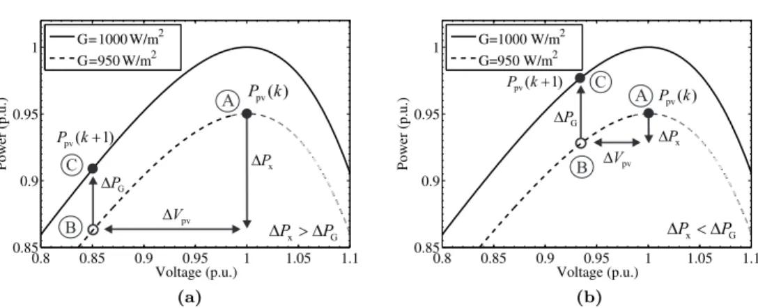
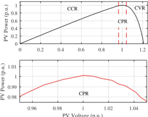
Perturbation step size cannot be reduced to an arbitrarily low value due to varying irradiance and noise in the measurement circuit affecting the accuracy of two consecutive PVG-power measurements. The erratic operation of the perturbative algorithm under varying irradiance condition can be explained by inspecting Fig. 1.9a, where the present operating point is at point A, and the sign of the next perturbation step is leftwards, i.e., to lower voltage level. If irradiance is increasing during the MPPT perturbation period, the new operating point moves from A to C instead of A to B. However, this is not a problem, since the power change caused by the perturbation is larger than the power change caused by the irradiance change corresponding toPpv(k+ 1)−Ppv(k)<0. Therefore, the sign of the next perturbation is inverted, i.e., the voltage is increased and the operating point converges towards the MPP. In contrast, the false response to the changing irradiance condition is illustrated in Fig. 1.9b. The starting point is the same as in Fig. 1.9a, the operating point is located at point A, and the sign of the next perturbation is leftwards. Due to the changing irradiance level between the perturbation periods, the operating point is moved from A to C. In this case, the sign of the next perturbation is calculated as Ppv(k+ 1)−Ppv(k) >0 and the direction of

next perturbation is leftward indicating the wrong operation of the MPPT algorithm. Such behavior will occur as long as the irradiance transition lasts, and eventually, the operating point will move towards OC or SC condition. In order to prevent such behavior, the perturbation step size should be designed to be high enough to provide power change in PVG terminals to overcome the power change caused by the irradiance variation within the same time interval as stated in [57].

In addition to fast-changing irradiance, different noise sources affect the operation of the perturbative algorithms. The most significant ones are the switching ripple noise, the measurement errors, the errors in numerical elaboration, and the output voltage noise [18]. As a consequence, the computed PVG power may not correspond to the real PVG power yielding an unpredictable operation of the MPPT algorithm. Thus, to guarantee the operation similar to represented in Fig. 1.8, all the noise sources that can affect PVG power should be analyzed and increase the perturbation step size ∆xcorrespondingly. Each noise source needs to be studied separately and their effect is added together to achieve the minimum required perturbation step size [18].

pv V D

(a) (b)

Fig. 1.9: Demonstration of (a) proper operation and (b) false operation of perturbative algorithms in fast-changing irradiance condition. [58]

Despite the fact that the effect of minimum perturbation step size is widely recognized in the literature, the upper limit also exits as recently revealed in [59]. That is because an open-loop and closed-loop interfacing converter may operate with relatively low damping factor, which causes oscillation during the transients. The undamped resonant behavior introduces overshoot also in the transient behavior of the inductor current. Therefore, if the perturbation step size ∆xis too large, the inductor current can move from continuous conduction mode (CCM) to discontinuous conduction mode (DCM). That transforms the second-order system into an equivalent first-order dynamic system extending the PV-power settling time significantly, thus, reducing power tracking performance and violating the validity of the theory to compute the power settling time in the previous studies [57, 60, 61], which will be further discussed in Section 4.4.

Adaptive and variable-step algorithms are introduced to overcome the trade-off sit-uation between the steady-state oscillation and fast dynamics in fixed-step perturbative algorithms. The conventional concept of an adaptive-step algorithm is based on varying the step size of the perturbation while the perturbation frequency is kept constant. Basi-cally, the algorithm adjusts the step size ∆xdepending on how far the operating point is from the MPP. When the present operating point is far from the MPP, a large step size is used to achieve the MPP faster. In contrary, a small step size is used when operating near the MPP to minimize steady-state oscillations. In order to calculate the value of step size, the power-voltage derivative ∆Ppv/∆Vpvis typically chosen as a suitable parameter for tuning the step size [62] since its value reduces when the operating point moves towards the MPP yielding ideally zero at the MPP. The main problem with the algorithm is to find a suitable scaling factor for ∆Ppv/∆Vpv and the minimum perturbation-step-size limits in order to satisfy the constraints discussed before.

Fig. 1.10: Simulated operation of adaptive-step MPPT (red line) and fixed-step MPPT (black line) under trapezoidal irradiance profile shown on the bottom figure [58].

Adaptive-step P&O algorithms are very sensitive to drift due to the derivate-dependent perturbation step size. Figure 1.10 highlights the problems with variable-step algorithms originally published in [58]. In the figure, fixed-step and adaptive-step P&O algorithms are compared to varying irradiance profile shown in the lower figure. Based on the sim-ulation in Fig. 1.10, the varying irradiance causes the algorithm to drift on both sides of the MPP with unpredictable behavior. In contrast, the perturbation step size in the fixed-step MPPT algorithm is chosen large enough to compensate irradiance variation, and therefore, the MPPT control operates with the basic three-step behavior. Therefore, as concluded in [58], the adaptive-step MPPT algorithms are very sensitive to noise, and therefore, additional mechanisms should be added to the algorithm to prevent drift phenomenon.

The second design variable of the perturbative algorithms is the perturbation fre-quency, i.e., the period between two consecutive perturbations. As Fig. 1.8a indicated, the undamped converter topologies exhibit resonant behavior in the transient conditions, which extends the settling process of PVG voltage and current also affecting PVG power. Therefore, the perturbation period ∆T should be longer than the longest settling time of the PVG output power transient induced by the injected perturbation, i.e., ∆T > T∆

must hold throughout the whole operation range, otherwise the algorithm may fail and the operating point can enter into chaotic behavior and lose its predictability [57]. As can be seen from Fig. 1.8a, the transient behavior changes according to the operating point. Thus, all operation regions should be studied to determine the conditions, where the settling time is the longest.

Even though different MPPT algorithms have been widely studied in the literature, their dynamic behavior is mostly neglected. The first detailed studies regarding the

optimization of the P&O algorithm design parameters are presented in [57], where the authors generated a dynamic model for the PVG-interconnected boost converter in order to determine the minimum settling time to prevent the drift phenomenon. However, alternative approaches are also introduced. The authors in [63] recommended to use 1/10 of the input-voltage-feedback-loop crossover frequency as the base for computing the PV-power-settling time. However, as reported in [60], the settling time of the transient cannot be determined solely by the control bandwidth since the damping factor and the phase margin have also a great impact on the outcome. Later, a few other studies have given simplified guidelines to determine an optimized value for perturbation frequency and step size. For example, the authors in [64] suggested that the speed of the MPPT algorithm should be in the range of 0.1–1.0 % of MPP voltage per second in order to reach annual MPPT efficiency of 99.9 %. The other approaches have been introduced by the authors in [65] utilizing shorter perturbation period. In that case, the PVG power never reaches the steady state yielding chaotic behavior around the MPP. Despite the interesting approach, such a high-frequency perturbation cannot be used in multi-loop converter control scheme due to the constraints of control bandwidths between outer and inner control loops.

It must be emphasized that the design guidelines represented in [18] and [57] seem to be generalized and intended for both open-loop and closed-loop MPPT structures. Nevertheless, there is no evidence in the literature (including [18] and [57]) of applying these to systems employing closed-loop MPPT structures. For example, the authors of [26] recommend determining the minimum allowed perturbation period by means of simulations rather than analytically. Consequently, the thesis aims to fulfill the gap by demonstrating that in case the input-voltage feedback loop is properly closed, PVG-power-settling time would be independent of PVG dynamic resistance, thus being longest in CPR. Revealed analytical findings are experimentally validated by utilizing a PVG-interconnected dc-dc converter [66].

Although the perturbation frequency does not directly affect the tracking efficiency, it has a significant impact on the operation of the algorithm in steady state and dynamic atmospheric conditions. That is because the perturbation frequency defines the tracking performance (i.e., power ramp rate ∆Ppv∆T) under dynamic conditions together with the

perturbation step size. Thus, these two design parameters of the perturbative algorithm should be selected carefully by taking into account dynamic behavior of the interfacing converter, possible noise sources affecting the PVG-power measurements and varying atmospheric conditions under the worst case scenario.

1.5

Objectives and scientific contributions

This thesis discusses the dynamic characteristics and operation of MPP-tracking dc-dc converters, especially, on those parts that are valid for MPPT-control design by contin-uing the previous work around the subject in [67]. By analyzing the published research results, it can be concluded that the given perturbative MPPT algorithm design guide-lines were either insufficient or missing in some parts. As a consequence, revisited and new methods to analyze PVG-power transients in case of open-loop-operated and closed-loop-operated dc-dc converters were introduced. Studies were performed with a voltage-boosting dc-dc converter. However, the fundamental principles behind the developed methods will remain the same with other converter topologies. Thus, the results provide practical methods to estimate the factors affecting the PVG-power transient in order to facilitate the MPPT design process as well as the design of the interfacing converters.

The main scientific contributions of this thesis can be summarized as follows

• Providing an explicit formulation of PV-generator power dynamics when intercon-nected with a switched-mode dc-dc converter. It is shown that the operating point can move from CPR to CCR even during the steady-state MPPT operation, lead-ing to a longer PVG-power-transient-settllead-ing time than the one expected at MPP. Consequently, unlike stated in the design guidelines utilized so far, the perturbation frequency design of direct MPPT control must be accomplished for the worst-case operating point expected to be in the constant current region rather than at the MPP in the case of duty-ratio-operated converters.

• Providing revisited-perturbation-frequency design guidelines to be invariant to the PVG during the perturbation frequency design process. Once the operation in the constant current region is assumed as the worst-case operating point, it was revealed that photovoltaic-generator influence on the perturbation frequency value vanishes and the perturbation frequency could be computed based solely on the dynamic behavior of the duty-ratio-operated interfacing converter.

• It has been shown that the dynamic behavior of the input-voltage-controlled con-verter does not depend on the properties of the photovoltaic generator, contrary to the duty-ratio-operated MPPT converter. Consequently, the settling time is longest when the operating point resides in constant power region due to the be-havior of the PV-power settling process. Therefore, it is recommended to use the constant power region related equations to compute the settling time in the case of multi-loop MPPT structures employing inner input-voltage-feedback control.

• Introducing a method to estimate the transient behavior of input-voltage-feedback-controlled MPPT converters for two typical design cases by focusing only on the