Contents
1 Introduction
1.1 On the Cortex in General……… 2
1.2 Research Questions………. 2
1.3 Thesis Outline………. 3
2 Neuro-Anatomical Organisation of The Cortex
2.1 The Thalamus and the Spatio-Temporal Code………... 42.2 The Layered Structure and Intra-Cortical Communication……… 5
2.3 Thalamo-Cortical Connections and Layer IV……… 6
2.4 Layers I, II and III: Taking Context into Account………. 8
2.5 Layer V: Summarising the Result……….. 9
2.6 Layer VI: Temporal Dynamics and Noise Reduction………... 10
2.7 Summary of Principles……….. 12
3 A Generic Computational Model of a Patch of Cortex
3.1 The Input Layer………. 133.2 Layer A: the Elementary Feature Layer……… 14
3.3 Layers B and C: Gain Control by Expectation……….. 19
3.4 Layer D: Coarse Grained Output……….. 21
3.5 Layer E: Temporal Dynamics, Topographic Organisation and Noise Reduction 22
3.6 Summarising the Algorithm……….. 25
4 Experimental Results
4.1 Inducing Plasticity of Global Organisation through Axon Migration………….. 274.2 Formation of Receptive Fields……….. 28
4.3 Creating Lateral Connections……… 29
4.4 Temporal Dynamics……….. 30
4.5 Local Topographic Organisation and Abstraction……… 31
4.6 Noise Reduction……… 32
5 Conclusion
5.1 Discussion………. 33 5.2 Future Research……… 34 5.3 References………. 36Section 1: Introduction
1.1 On the Cortex in General
The rise of man is indisputably linked with the tremendous increase of his cortex-to-body ratio. This increase did not start with man, however, but with mammals in general. Over 195 million years ago the separation between mammals and mammal-like reptiles is presumed to have occurred, and since that time the cortex has grown drastically, indirectly implying its significance.
Reptiles possess a relatively small cortex for crude sensory analysis and primarily rely on the sub-cortical mechanisms of the mid- and hindbrain to guide behaviour. It is believed that decisions made by these areas can be considered 'instinctive', as it's possible to describe the resulting behaviours in terms of simple stimulus-response rules. Though mammalian behaviour is still guided by these primitive instincts (primitive in terms of their age in evolution), the expansion of the cortex gradually enabled an increase in the complexity of the emerging behaviour.
Where a reptile's decisions can often be explained in the context of the directly
observable world around him, with mammals this approach does not suffice. From the expansion of the cortex emerged a new tool for decision-making that evolved on top of the older system and enables mammals to 'think' beyond the here and now. In everyday speech we often refer to this tool as the faculty of reason.
Reason requires world knowledge, and it is the cortex that provides this. We need to extract the important facts from the information passed on by our senses, to evaluate these facts and decide what's important and what is superfluous. We normally tend to refer to reason as the manipulation of symbols in accordance with the rules of logic, but we often forget that reasoning need not be that abstract. While the use of symbols
requires high-level object recognition (and is inestimably enhanced by speech), 'common sense' reasoning as anticipating a tennis ball’s trajectory will find this symbolic type of little use. Reptiles’ small cortices seem to be capable only of this superficial sensory reasoning, providing them with enough mental power to catch and devour their prey. Abstract symbolic reasoning, however, is definitely beyond their capacity.
Although these types of reasoning may seem very different at first glance, they can be summarily classified as 'predicting a certain outcome'. This warrants the hypothesis that the differences in mental power may not need to be explained in terms of different mechanisms; applying the same principles at different levels of abstraction could do the trick.
1.2 Research Questions
The aim of this thesis is to explore the principles of a patch of cortex and how it deduces ‘what is out there’, predicts ‘what will be there’ and is capable of bringing about the higher levels of abstraction that endowed Man with his so-called faculty of reason.
1.3 Thesis Outline
This thesis is based on research conducted by the author during his half-year internship at the Artificial Intelligence Laboratory of the University of Zurich, Switzerland. Much of the credit goes to Dr. H. Valpola, responsible for the initial framework and direction of the research. Besides providing many of the ideas put forward in this thesis, he also proved to be a sparring partner invaluable for keeping the author's youthful enthusiasm in check. The main body of this thesis is divided into three sections:
1) Facts and Evidence from Biology 2) A Computational Model
3) Experimental Results
The first part provides a description of the findings of neuro-anatomic research, such as cortical organisation, the connections found between neurons and neurons' firing
properties. The second part proposes a model that tries to explain the emergence of these properties and to provide an understanding of why they are necessary. As its aim is to give insight into the functioning of the cortex, biological plausibility has been a chief requirement during its development. The last part shows the results of a software implementation of this model, programmed by the author in Matlab.
The views proposed in this thesis are the result of a synergy between the behaviour of this computational model and the biological findings by which it was inspired.
Section 2: Neuro-Anatomical Organisation of The Cortex
At cellular level the cortex is a very messy place, and to see structure among the
proliferation of seemingly random connections is an arduous job reserved solely for the most patient of researchers. It is thus unsurprising that when looking for a specific connection to prove a certain theory, chances are high supporting neurobiological evidence will be found.
For this reason, the approach used by the author when constructing a generic
computational model of the cortex was not to take each connection ever found seriously. Only when a significant number of researchers consistently reported finding a connection in multiple places on the cortex was it integrated into the model. The findings and their interpretation are presented below.
It must also be mentioned, however, that liberty has been taken to leave many types of cells and connections out of the discussion. This is not because they contradict the hypotheses presented below, but merely because they unnecessarily complicate matters and encumber understanding.
2.1 The Thalamus and the Spatio-Temporal Code
Except for the olfactory pathway, all sensory information is passed through the thalamus to the cortex, thereby providing the interface between the cortex and the rest of the body. Each sensory modality is allocated a separate part of the thalamus, being for instance the lateral geniculate nucleus (LGN) for the visual pathway and the medial geniculate nucleus (MGN) for the auditory pathway (figure 2.1).
Figure 2.1: sagital view of the brain (left) with enlargement of the thalamus (right)
Although the origin of the information passed through this brain structure is different for each modality, its nature is the same, namely spike trains (sequences of action potentials) conveyed by individual neurons. Yet, besides merely carrying information through the firing patterns of single neurons, groups of thalamic neurons also supply additional information through their relative spatial ordering. Examples of these are the retinotopic organisation of the LGN and the tonotopic organisation of the MGN (retinotopic implies
the retina, while tonotopic means that the frequency sensitivity changes gradually across the MGN). This type of organisation has the desirable effect that neighbouring thalamic neurons are in some way related, and results in all sensory information being encoded both in terms of temporal and spatial activation patterns.
Research has taught us that one of the cortex' prime functions is the recognition of relevant patterns and that the cortex is essentially a homogenous substance (M.
Merzenich and J. Kaas, 1980). Homogeneity implies a functioning according to similar principles regardless of modality, and thus standardisation of the code becomes essential. This requirement is fulfilled by encoding sensory information from all modalities not just in terms of neurons’ temporal firing properties, but also in their spatial organisation relative to each other.
2.2 The Layered Structure and Intra-Cortical Communication
One of the most salient characteristics of the cerebral cortex that is evident in all mammalian species is that most of it is made up of six layers (figure 2.2). These layers are organised in cortical vertical columns (CVCs), with each column forming a functional unit spanning all layers. The net flow of information through these CVCs starts in layer IV, where afferent axons from the thalamus make connections with small interneurons. These interneurons in turn project to layers II and III where they excite pyramidal
neurons, the most common type of neuron found in the cortex. The pyramidal neurons in Layers II and III then proceed to excite other pyramidal neurons in layers V and VI, who send their axons outside of the cortex. It is important to note, however, that this is a simplified model of the flow of information, and that in practice evidence exists for connections linking almost every layer.
Figure 2.2: laminar organisation of a cortical column. Left: stain showing 2% of neurons, middle: stain showing only cell bodies, right: stain showing only axons.
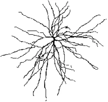
The cerebral cortex functions in such a way that the neurons inside a CVC have a limited receptive field (range of stimuli able to excite the cell) and are selectively responsive to specific inputs within this field. For V1, the primary visual cortex, these have been found to be predominantly line segments of different orientations coming from a small part of the retina (D. Hubel, T. Wiesel, 1968), while for A1, the primary auditory cortex, these
are specific frequencies. The average pyramidal neuron in the cortex does not exceed its base firing rate 99.8% of the time (R. Desimone, 1998), which fits nicely with the idea that a CVC only becomes active when its preferred input is presented.
2.3 Thalamo-Cortical Connections and Layer IV
The afferent axons from the LGN sprout broad axonal arbors that form excitatory
connections with very small but densely packed stellate interneurons in layer IV (figures 2.3 and 2.4). With an average diameter of 1.5mm in V1 (S. Hill and G. Tononi, 2001), these arbors are quite large, effectively spreading their information over a large area (M. Bickle, 1998). This extra space is essential for CVCs to develop.
Figure 2.3: spiny stellate cell Figure 2.4: thalamo-cortical connections to layer IV
Though the axonal arbors are wide and overlap each other, the arbors are still limited in range and are themselves topographically organised. This organisation is therefore maintained in the cortex. However, due to the spreading of information it is not as exact as its thalamic counterpart, yet enough to identify, for example, a clear retinotopical organisation in V1.
Presumably these axonal arbors form very specific connections with particular stellate neurons. This specificity is not predetermined, but instead appears to be the result of a pruning mechanism based on Hebbian learning. Thus, though in early life layer IV stellate cells may be responsive to any stimulation within their receptive field, each neuron gradually learns to become maximally active only when a specific axonal input pattern is presented. As already mentioned, in the primary visual cortex this is often a line of a certain orientation and at a very specific place of the retina (figure 2.5).
Figure 2.5: idealised effect of pruning on the receptive field of a layer IV stellate cell
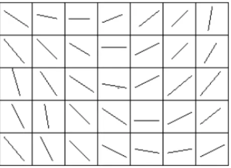
Aside from their input selectivity, another important property of layer IV neurons is that across the cortical plane these selectivities are topographically organised. It thus happens to be that neighbouring layer IV neurons have related input preferences, resulting in the gradual change of orientation preference found in V1 (figure 2.6). The mechanism(s) defining this 'relatedness' is not yet fully understood, but a plausible candidate is the temporal separation normally occuring between patterns. From this viewpoint, lines whose orientations differ only a few degrees are not more related than those differing 30 degrees because of the amount of degrees of separation, but because they are more likely to occur one after the other close in time (as in a line gradually changing orientation). The advantage of this principle is that it can be used for every modality, and not just the visual one.
Figure 2.6: idealised topographical organisation of orientation sensitive neurons in layer IV of V1.
Finally, within layer IV an abundance of short-range inhibitory connections between stellate neurons has been consistently found (S. Grossberg, 2001). It is expected that these strongly contribute to the sparsity of activation found in the cortex, as all active neurons inhibit their neighbours (figure 2.7) and hence only those with the strongest activations remain active. This can be viewed as a competition mechanism for activation with a 'local winner wins all' strategy.
Figure 2.7: idealised lateral connections in layer IV
To sum it all up, we can consider the thalamo-cortical connections, the layer IV stellate neurons and their inhibitory interconnections to implement an elementary feature extractor. Each stellate neuron represents a specific feature that is determined by the strengths of the thalamo-cortical connections, and the cells’ activations are a measure of the degree to which these features are present in the input. Local inhibition allows only the most salient features to remain active. How these thalamo-cortical connections (i.e. features) may be learnt will be discussed in section 3.2.2.
2.4 Layers I, II and III: Taking Context into Account
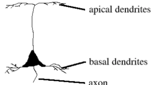
Each layer IV stellate neuron sends its axon up to layer III, where it connects with the basal dendritic arbors of pyramidal neurons (K. Catania, 1995). The connections between layer IV and layer III neurons are probably very local, resulting in an almost one-to-one relationship between them (figures 2.8 and 2.9). For this reason, the bottom-up inputs into layer III may very well copy the layer IV activations onto layer III.
Figure 2.8: a pyramidal neuron Figure 2.9: bottom-up input from layer IV to III
It is probable that the real added value of layer III doesn't lie in its connections with layer IV, but in those it maintains with layers I and II. Long-range lateral axons originating from layer III pyramidal neurons excite layer II stellate neurons far away (figure 2.10) and appear to link CVCs with input pattern preferences that are somehow related (U. Polat, 1996). It would thus be expected (and has also been proven) that unlike the connections with layer IV these long-range connections depend heavily on learning (Durack and Katz, 1996). This will be further discussed in section 3.3.3. The distances travelled by these axons may (again) be as much as 1.5mm in V1 (R. Miikulainen, J. Sirosh, 1996) where they predictably connect CVCs responsive to lines of similar orientation that lie in each other's extension.
Figure 2.10: long-range lateral connections from pyramidal neurons in layer III to stellate cells in layer II. The latter send their axons straight up to layer I, where they hatch onto the apical dendrites of layer III neurons.
The layer II stellate cells project in turn to layer I, which contains no cells; only the apical dendrites of layer III pyramidal neurons. These connections have been found to be both excitatory and inhibitory (M. Usher, 1996). Important to observe is that on average apical dendrites are found much further from the cell body than the basal ones. This would result in basal input having a much directer and stronger influence than apical input. Layer II activation is, however, very capable of facilitating layer III, which justifies the assumption that basal stimulation is driving while apical stimulation is modulatory. The main purpose of these excitatory and inhibitory lateral connections may be to
Although the exact functioning of this mechanism is still unknown, neurons connected by these lateral connections were found to sometimes excite, and sometimes inhibit each other. It is hypothesized that Layer II brings about an expectancy measure for a specific layer III neuron, being more expected with more lateral input. This expectancy could in turn be used to alter the saliency of an extracted feature: if the feature is expected but bottom-up evidence is weak (perhaps due to poor lighting conditions), the feature would be enhanced. If, on the other hand, the bottom-up evidence is strong it would be useful to suppress it, allowing other unexpected features to pop out.
2.5 Layer V: Summarising the Result
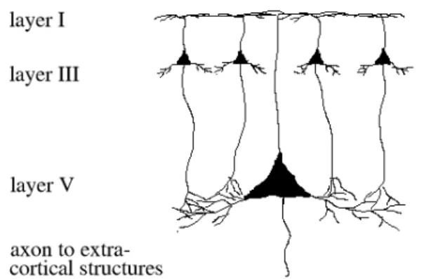
Layer III sends its axons to layer V where they hatch on to the basal dendrites of pyramidal cells (figure 2.11). Layer III thus seems to provide the driving impetus for layer V. Layer V cells also have larger cell bodies than those of any other layer (figure 2.2), and as a result fewer can be found. Not much is known about the specificity of these connections, but putting the above facts together leads one to believe that layer V
summarises the activation within a neighbourhood of layer III cells. Because of the topographical organisation of layer III, this summary would still contain plenty of information in order to be useful.
Figure 2.11: driving connections from layer III to layer V
On the purpose of such an information reduction one can only speculate. Considering layer V is the principle output layer to extra-cortical structures, its coarse resolution may be preferential to these structures than the fine-grained version of layer III. Another advantage would be that it reduces the amount of outgoing axons, which is crucial if we wish to keep the output size (number of layer V pyramidal neurons) equal to the input size (number of thalamo-cortical axons). Failure to do so would lead to an undesirable non-linear expansion in the amount of required cortex space at higher levels.
Finally, by summarising layer III activation it is probable that layer V will be more invariant than layer III, being responsive to a whole range of patterns instead of
individual ones. In section 5.2 hierarchies of cortical maps will be considered, and here it will become apparent why this invariance is necessary to attain stable object recognition.
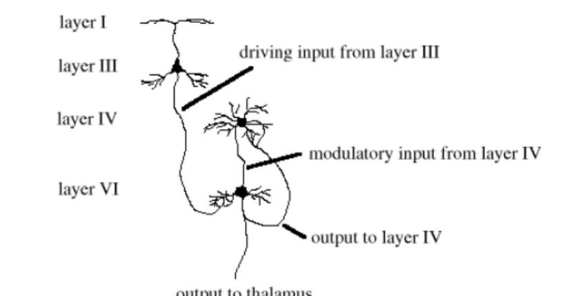
2.6 Layer VI: Temporal Dynamics and Noise Reduction
Layer VI contains a wide variety of cells, all of which presumably have different
functions. Due to the inward position of this layer it has been difficult to study these cells in detail, but hypotheses on some of their functions exist.
First of all, small pyramidal cells are found that have their basal dendrites stimulated by layer III neurons. They thus rely on layer III to provide the driving input, while their apical dendrites are usually found in layer IV (K. Catania, 1995, see figure 2.12). Though apical stimulation alone won’t lead to an action potential, they heavily facilitate their layer VI pyramidal cell’s firing probability when basal stimulation is present. Layer VI pyramidal cells tend to send their axons directly up to layer IV, but many also project back to the thalamus.
Figure 2.12: connections to and from layer VI
2.6.1 Temporal Dynamics
One of the functions of these cells may very well be the introduction of temporal
dynamics into the cortex. It takes time for activation to be propagated through the entire CVC and this delay can be exploited for learning activation sequences on layer IV. Temporal context would suddenly become a factor, enabling properties like the direction sensitivity in addition to just the orientation sensitivity of V1 cortical neurons. Hawker, Parker and Lund support this view, claiming they found that layer IV neurons loose their direction sensitivity when layer VI is knocked out (Hawker, Parker, Lund, 1988). A hypothesis explaining these findings may be as follows. An active layer IV neuron would trigger the layer III neuron within the same CVC. This layer III neuron would in turn excite a layer VI neuron outside (but close to) it’s own CVC. This layer VI neuron would then proceed to facilitate the layer IV neuron of its CVC, which is therefore a different one than the layer IV neuron that started the cascade.
By the time this loop has been completed the thalamic input into layer IV will probably have changed (the line in the picture will have moved, or the pitch in the melody will have shifted etc.). However, the layer III-to-VI connection will be such that, considering the previous input, the CVC newly facilitated by layer VI is the one expected to be activated next. Given sufficient supporting thalamic evidence for this newly facilitated
layer IV neuron (or lack of conflicting information), the additional temporal facilitation would insure that that CVC indeed wins the local competition in layer IV.
Because a different input history means different layer III neurons were previously active, this would also imply that probably different layer VI neurons were active as well. In V1’s case this means that although the thalamic input may be the same (a line at a certain place of the retina), it is the facilitation of layer VI that provides the temporal information as to whether this line is moving left or right. This layer VI facilitation leads to the activation of different layer IV neurons depending on the direction of movement. 2.6.2 Topographic Organisation
Another function of layer VI may be to induce the topographical organisation of gradually changing receptive fields of layer IV. Although no supporting biological evidence has yet been found, it would not be too unlikely if instead of very specific 1-to-1 connections, layer III axons actually sprout small axonal arbors in layer VI. This would link each layer III neuron to a small layer VI neighbourhood, which in turn modulates a small neighbourhood on layer IV. How this could aid topographic organisation will be discussed in section 3.5.2.
2.6.3 Noise Reduction
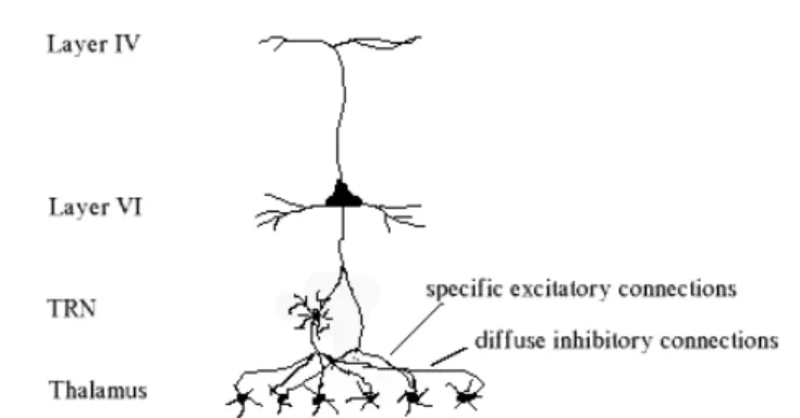
But besides projecting up to layer IV, layer VI neurons also send axons back to the area of the thalamus from which they receive their information in the first place (S. Luck, 1997). Here they form direct excitatory connections with neurons in the thalamus and the thalamic reticular nucleus (TRN). Where the direct cortico-thalamic connections are very specific, neurons excited in the TRN in turn have a diffuse inhibitory effect on the
thalamus (figure 2.13).
Figure 2.13: cortico-thalamic connections
It is believed that within the thalamic cells excited directly by the layer VI neurons, the excitatory and inhibitory influences are roughly equal and therefore cancel each other out (Grossberg, 2002). On the other hand, the effect on those thalamic neurons that are not directly excited by layer VI but lie close to those that are, the diffuse inhibition from the TRN is still present and consequently suppresses their activations. This view is supported by the fact that stimulation of layer VI alone rarely leads to thalamic activation, but when bottom-up input into the thalamus is present, layer VI is quite effective at diminishing the activation that’s already there (S. Luck, 1997). Considering these facts, noise reduction
would seem a likely candidate for the function of these connections, a hypothesis that will be further discussed in section 3.6.
2.7 Summary of Principles
Considering the facts and views presented in this section, a summary of the important (yet hypothetical) principles applicable to the cortex in general may be as follows:
- Spatial patterns are extracted using the thalamic receptive fields of layer IV. These receptive fields arise due to the specificity of thalamo-cortical connections. - Temporal patterns are also extracted by layer IV, but with the aid of layer VI. The
delay of layer VI compared to Layer IV enables layer IV to ‘remember’ what happened at an earlier time.
- The organisation of CVCs (such as the gradual change of orientation-selectivity in V1) is decided by temporal properties of the input patterns only. The fact that CVCs with similar spatial receptive fields are located close by is only because these patterns often occur close in time.
- Layers I, II and III implement a mechanism in which the local patterns extracted by layer IV are compared with what is known on a more global level and adapted accordingly. Thus, depending on what other pieces of the cortex ‘know’, extracted features may be either suppressed or made more salient.
- Layer V summarises what the cortex has calculated, thereby reducing the amount of output information and introducing the invariancy (or abstraction) needed for higher-level cognition (see section 5.2).
- Besides introducing temporal dynamics, another function of layer VI may noise reduction in the thalamus. This may be closely linked with attentional
mechanisms.
Section 3: A Generic Computational Model of a Patch of Cortex
Neuro-anatomic research has given us in-depth knowledge of the cellular organisation of the cortex and the complex connectivity within and between layers. Due to this
complexity, however, it is very difficult to discover important underlying mechanisms from neurobiological data directly. For this reason, instead of observing what the cortex does in practice, it may be more fruitful to hypothesize about how the cortex could work in theory. This means abstracting from the myriad of cell types and their connections and proposing a biologically plausible model that gives rise to the same properties as the real cortex.
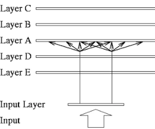
The model presented in this chapter retains the laminar organisation present in the actual cortex, but to avoid confusion the following translation is used:
Brain Model Thalamus Input Layer Layer IV Layer A
Layer III Layer B Layer II Layer C Layer I NA Layer V Layer D Layer VI Layer E
Layer I contains no neurons and consequently lacks interesting computational properties. For this reason it is not modelled.
3.1 The Input Layer
The cortex receives input from the senses, and the obvious counterparts for our model would be artificial sensors like cameras and microphones. The information sent by these sensors is copied onto the input layer, which has the same function as thalamic nuclei like the LGN or MGN. Thus, for a camera sending 32x32 greyscale pixel images the input layer would be a 32x32 matrix with values ranging from 1 to 256, each entry
corresponding to the intensity of a pixel.
It is important to note that whatever the source of information, for the system to function properly the values in the input layer have to be strictly non-negative. This is perfectly defendable, considering each entry value is the computational equivalent of the intensity of a spike train. And how could a burst of action potentials have a negative frequency? Besides being a relay site for sensor data to layer A, the prime function of the input layer is to form part of a greater denoising mechanism. The functioning of this mechanism, however, will be discussed in section 3.5.3, when we’ve also considered layer E.
3.2 Layer A: the Elementary Feature Layer 3.2.1 Propagation of Activation
Layer A also consists of a 2D matrix of artificial neurons and its values correspond to the stellate neuron activations of layer IV. It receives its input primarily through the
connections it enjoys with the input layer. As with normal neural networks, these
connections have different weights, and the layer A activations depend on the input layer activations multiplied by the weights between the input layer and layer A (see formula (1) and figure 3.1).
Aa = WIa*AI (1)
where Aa = activation of layer A neuron 'a'
WIa = weights between the input layer neurons and 'a' AI = the input layer activations
As mentioned in chapter 2, the direct thalamo-cortical connections to layer IV stellate neurons have been found to be excitatory, and for our model this translates into the existence of only non-negative weights.
Figure 3.1: Cross-section of the propagation of information from the input layer to layer A. In reality all layers are 2D and the branches from the input layer to layer A can be considered as cones.
3.2.2 Weight Learning
We hypothesized that the connections between thalamo-cortical axons and layer IV stellate neurons are very specific, enabling layer IV neurons to develop highly distinctive receptive fields (figure 2.3). As with all neuronal learning, the mechanism leading to this organisation should primarily be based on Hebb's law, which states that the connection between two neurons is strengthened only when both neurons are active at the same time. Another important learning principle found throughout the nervous system is that when a post-synaptic neuron is active without its pre-synaptic counterpart being so, the
connection between them is weakened. This type of learning can easily be implemented with the following formula:
δWia = Ai*Aa – C*mean(AI*S(Ia)) (2)
Aa, Ai, AI = the activities of neuron 'a', neuron 'i', and the input layer respectively C = a constant, in our implementation 0.1
S(Ia) = the set of all activations of input layer neurons that form connections with neuron 'a'
AI*S(Ia) = the members of the set S(Ia) multiplied by their activations The term Ai*Aa in (2) simulates Hebb's law and causes the weight change to be proportional to the combined activity of both the layer A and the input layer neuron. Since all input layer activities are positive and the connections between the input layer and layer A are positive as well, Aa will also always be positive and so will Ai*Aa. This means that the term Ai*Aa can only strengthen connections.
The term C*mean(AI*S(Ia)), on the other hand, is used for the second learning principle and represents the average Ai*Aa value for a particular layer A neuron. Input layer activations that haven't contributed much to the excitation of neuron 'a' have a lower than average Ai*Aa value and hence formula (2) may cause their weight changes to become negative (also depending on C).
If the new weight of such a connection is negative, it is set to 0 (see formula (3)). This satisfies the constraint that only non-negative connections are allowed and, as we'll see below, has additional advantageous side-effects.
Wia = rect(Wia + δWia) (3)
where Wia = the connection weight between neurons 'i' and 'a' rect = a function that changes any negative number to 0 3.2.3 The Neighbourhood function
In chapter 2 we saw how thalamo-cortical axons sprout broad axonal arbors that form connections with many stellate neurons within a certain neighbourhood. This localised arborisation principle is simulated in the model by pruning the connections between the input layer and layer A. Towards this end, the centre of mass of weights sprouting from each input layer neuron with respect to layer A is calculated. Then, on layer A a pre-specified maximum arbor radius with this centre of mass as its centre is used to define the axon's neighbourhood, outside which a connection is pruned.
One must bear in mind, however, that despite this inability to form connections beyond a neighbourhood, within it the weights of the connections are allowed to change, hereby possibly displacing the axon's centre of mass and allowing the neighbourhood to migrate across layer A (figure 3.2). In section 4.1 we will see how this migration allows axons that convey information somehow correlated to move closer to one another and project to the same layer A neurons. This is essential for useful receptive fields and global
Figure 3.2: cross-section of input and layer A demonstrating the migration of an axonal arbor
Thus, given an input layer neuron and its outgoing weights, we may define the neighbourhood as follows:
NHi = (1 – Disti/ArborRadius) > 0 (4)
where NHi = the neighbourhood of an input layer neuron 'i'
Disti = the distance of a point on layer A to the centre of mass of weights sprouting from 'i'
ArborRadius = the pre-specified radius of axonal arbors
This formula describes an inverted parabola whose non-positive values are set to 0, while its remaining values are set to 1. This leaves a disc of ones amidst a plain of zeros. NHi is then multiplied with the connection weights, pruning any connections forming outside this neighbourhood. New connections are given the strength ε, a very small (but non-zero) positive number. The advantage of using these neighbourhoods is two-fold: 1) The computational complexity (amount of weights) scales linearly with the input size
and the arbor radius. It is unaffected by changes in the size of Layer A.
2) It enables parallel local processing of large amounts of data, as information of an axon is only distributed as far as the axon's neighbourhood. This becomes especially useful in combination with a hierarchy of cortical maps, which will be discussed in section 5.2.
3.2.3 Global Competition for Weights
The danger of using migrating local neighbourhoods is that layer A neurons that should receive information from a certain group of input layer neurons (perhaps because these input layer neurons contain information from the same site of the retina) in fact don't, due to different neighbourhoods having migrated too far from each other. In other words, there has to be some driving force that organizes the neighbourhoods among each other, grouping those that are statistically related close together and separating unrelated ones. In our model, this driving force is provided by divisionally normalising the total sum of
layer neuron, this means it can establish connections of strength 1 with all layer A neurons within its neighbourhood. If you have many input layer neurons with their neighbourhood covering the same layer A area, however, that means they'll have to share their weights with others (since the sum of weights leading into one layer A neuron is maximally 1).
WIa = WIa / (sum(WIa)) (5)
where WIa = the connection weights from the entire input layer to a layer A neuron 'a' On the other hand, nothing bounds the sum of connection weights per input layer neuron (or in other words: the sum of axonal arbor weights) and each individual weight of an arbor can therefore still be 1, irrespective of the presence of other neighbourhoods. When a connection between an input layer neuron and a layer A neuron is 1, this means that the input layer neuron has exclusive control over the firing properties of the layer A neuron, as that neuron gets no input from other input layer neurons.
Now, if outside this crowded neighbourhood there are few other arbors competing for weights to layer A neurons, this means that any axon can more easily establish large weights in these less competitive regions. If given this possibility, the axon will of course do so, shifting the centre of mass in the process and displacing the neighbourhood
towards this less crowded area. The net effect is that arbors will migrate along a gradient of decreasing crowdedness which, given enough layer A space, would eventually result in a distribution of axonal arbors across layer A where no overlap between arbors occurs. In this case no layer A neuron would receive input from more than one input layer
neuron, and this is of course undesirable as it is exactly our intention for a layer A neuron to receive information from a number of neurons. To achieve this, we simply limit the size of layer A and force the axonal arbors to overlap. The arbors will still try to obtain as many strong connections to layer A as possible, and the resulting dynamics can be
described as the arbors following a path of least resistance until they finally reach a stable distribution.
If the repulsive force between axons would be the same for everyone, this would just lead to an equal spread of the arbors over layer A without grouping statistically correlated arbors together. There exists, however, a crucial difference between the repulsive force of different axonal arbors. Namely, correlation between input layer neurons means that these neurons are often active at the same time. These active neurons will activate layer A neurons within their neighbourhood and the Hebbian learning rule will strengthen their connections. Hence, correlated axons with an overlapping neighbourhood will make strong connections with the same neurons, while on the other hand inactive axons will find their connection weights reduced as a result of the divisional normalisation. These weight changes will have effect on the centres of mass, strongly repulsing the
neighbourhoods of inactive axons away from active layer A areas.
This can be summarised by stating that all arbors repulse each other, but some repulse more than others (namely the uncorrelated ones), and this is what leads to the global organisation of axonal arbors. It could very well be possible that it is this mechanism that leads to the retinotopical organisation found In V1.
3.2.4 Local Competition for Activations
Although this global competition mechanism is able to induce a topographical ordering between different axonal arbors, it has no control over what happens at a more local level, namely within these arbors. First of all, in order to obtain the invariances needed for stable object recognition (section 5.2) we'd like neighbouring layer A neurons to represent related but distinctive features, leading to topographic organisation like the gradual change of orientation specific CVC's in V1. Also, if we'd simply propagate the input layer activations to layer A, most layer A neurons would at least have some activation, making it indeed difficult to decide which features in the sensor data are the most salient. Preferably, only those layer A neurons responsive to the most salient features should remain active.
A way to enforce this is to introduce a competition mechanism that, instead of competing for weights like the global competition mechanism, would compete for activations in layer A. It may very well be that the inhibitory lateral connections in layer IV mentioned in section 2.3 have exactly this purpose, decreasing activation of most neurons within a certain radius while leaving only the strongest excited. Since learning is activation
dependent, if we make the competition strong enough (i.e. only one winner within a small area) this means that neurons close by are unable to learn the same features. In the model, this mechanism is simulated by the following formulas:
AA = rect(AA – smooth(AA)) (6)
AA = AA/(C + smooth(AA)) (7)
where AA = the activations of layer A
smooth = a function that spreads the activation of its argument in a normally distributed manner
C = a constant, in our implementation 0.1
Formula (6) implements a form of subtractive normalisation, filtering out lower than average activations. Since (6) has a strong reducing effect on most of the activations, some compensating factor is needed to allow the remaining activations to recover. Formula (7), a form of divisive normalisation, is used towards this end (Figure 3.3). The constant C is added to prevent small activations from being boosted to activations that are too high.
Care is also taken that after formula (7) no activation exceeds the value of 10. There are many ways of enforcing this, and therefore the specific formula has not been included here. This procedure of consequent subtractive and divisional normalisation may be applied a number of times to achieve the desired sparsity of activations.
Since weight learning is activity dependent and neighbouring neurons are rarely active at the same time, the effect of local competition is to de-correlate neighbours. Although this satisfies the requirement of neurons having distinctive receptive fields, organising these receptive fields in a topographic manner is still not achieved. As we'll see in section 3.5.2, layer E will be responsible for this.
3.3 Layers B and C: Gain Control by Expectation 3.3.1 Propagation of Activations
As was mentioned in section 2.3, evidence exists that the long-range excitatory lateral connections found in layers II and III implement a gain control mechanism. We saw that between CVCs with related receptive fields reciprocal connections have been found, and that these are presumed to create lateral circuits across the cortical surface (see figure 3.4).
Figure 3.4: left: propagation of layer A to B, middle: propagation of layer B to C through long-range lateral connections, right: propagation back from layer C to B
Provided enough neurons within such a circuit are active, these could selectively suppress or facilitate other circuit members. The result is that, given enough lateral supporting evidence, a layer B neuron with weak activation may be elevated to a higher excitation level, while highly active neurons’ activities are reduced. This mechanism may be implemented by the following formulas:
Ab = Aa (8)
Ac = WBc*AB (9)
Ab = Ab + (Ab>0)*(0.1*Ac)*(3-Ab) (10)
Where Aa, Ab, Ac = the activations of a layer A neuron ‘a’, a layer B neuron ‘b’ and a layer C neuron ‘c’ respectively, each lying directly above the former WBc = the (positive) weights from layer B into ‘c’
AB = the layer B activities
Formula (8) models the driving bottom-up input from layer A into layer B. In section 2.4 the propagation of layer A to B was hypothesized to be very local, resulting in the
copying of layer A onto B. Next, (9) simulates the propagation of layer B to layer C using the long-range lateral connections. Finally, each layer C neuron’s activation is used as an ‘expectation’ measure for the layer B neuron directly below it and (10) alters it
accordingly. Formula (10) works as follows:
- (3-Ab) is the term deciding the change of Ab (whether it’s tuned up or down), where 3 is the target value.
- Since Ac is between 0 and 10, (0.1*Ac) is between 0 and 1 and can be seen as a throttle for the amount of influence of Ac on Ab. If Ac is 1 (i.e. Ab is fully expected), Ab is changed to the target value of 3, while if Ac is 0 Ab remains unchanged.
- (Ab>0) enforces the fact that layer C is only allowed to have modulatory influence on layer B; expectation alone is not enough, at least some bottom-up evidence must be present to generate layer B activation.
The resulting effect of layer C on B is as follows: Layer A Evidence Layer C Expectation Layer B Modulation
Weak Strong Facilitation
Strong Strong Suppresion Weak Weak None Strong Weak None
The advantage of this mechanism is that in situations where bottom-up sensory input is weak, expectation in the form of lateral input may enhance the perceptional process. On the other hand, when sensory stimulation is sufficiently strong, there’s no need for all the neurons that were predicted anyway to retain their high level of activation. In fact, by reducing the activation of expected neurons while letting the unexpected ones go unsuppressed, the latter will ‘pop out’ compared to the former. This way, unexpected patterns become more salient than the expected ones and the system is made sensitive to novelty (or unexpectedness).
3.3.2 Creating Lateral Connections
Whether in the brain the lateral axons from layer III pyramidal neurons grow gradually outwards or whether they exist beforehand and are consequently pruned is still unknown. The answer is probably a combination of the two, but happens to be of little importance to us since the end result would be the same whatever strategy is used. For the model, the pruning approach would mean creating a great many redundant connections, slowing down the system needlessly. From a computational efficiency perspective, it would therefore be better to start with no lateral connections and only connect those neurons that are potentially related. This is implemented as follows:
1) Initially, each layer B neuron excites the layer C neuron straight above it. This corresponds to strictly vertical connections of strength 1 and means layer B is merely copied onto layer C.
2) For consequent iterations of the algorithm:
2.1) First, the probability is calculated for an active layer B neuron to form a connection with an active layer C neuron. These probabilities depend on the activity of the layer B neuron and the activity of and the distance to the layer C neuron:
P(Cbc) = (Ab*Ac)/(C*Distbc) (11)
Where P(Cbc) = the probability of forming a connection from a layer B neuron ‘b’ to a layer C neuron ‘c’
Ab, Ac = the activities of ‘b’ and ‘c’ respectively C = a constant, 10 for our implementation
Distbc = the distance between ‘b’ and ‘c’
2.2) A random number between 0 and 1 is assigned to each probability. If the random number is lower than the probability, the very small number ε is added to the weight between the respective neurons. For new connections this would mean a connection of strength ε is created where previously the strength was 0, while for existing connections the increase is insignificant.
3.3.3 Weight Changes of Lateral Connections
Like all learning in the brain, the changes in connection strength should be based on Hebbian learning. For the model, this implies that weight learning for lateral connections uses the same mechanism as the thalamo-cortical connections and which is described by formulas (2) and (3). Thus, as a quick reminder, weight strenghtening results from the co-activation of two neurons, while weight weakening occurs when the postsynaptic neuron is active without the presynaptic neuron being so. Also, weight changes between
connections with strength 0 (i.e. no connection exists) are not allowed, similar to the way a weight change with a layer A neuron falling outside the neighbourhood of a thalamo-cortical axon is treated.
Just like with thalamo-cortical connections, the total strength of connections entering a layer C neuron is normalised to 1 (formula (5)). The result is that layer B neurons exciting a layer C neuron compete with each other for access to this neuron and that the layer B neuron originally enjoying complete control over ‘his’ layer C neuron will gradually be forced to share its influence.
3.4 Layer D: Coarse Grained Output
Layer B’s final analysis is passed onto layer D, which is the principal output layer and corresponds to layer V in the cortex. As we saw in section 2.5, layer V contains bigger and fewer cells than any other layer and is therefore hypothesized to contain a low-resolution representation of layer III. For our model this translates into a smaller matrix
than the ones used for layer A, B and C, with each entry representing a local average of layer B activity. The formula of this conversion is:
AD = fixedSample(smooth(AB)) (12)
where AD, AB = the activities of layers D and B respectively
fixedSample = a function that takes a matrix, reads out values at regular intervals and returns them in a smaller matrix
Because layer B is first smoothed before it is sampled, layer D indeed stores a local average of layer B (figure 3.5).
Figure 3.5: the local averaging of layer D
3.5 Layer E: Temporal Dynamics, Topographic Organisation and Noise Reduction Communicating information takes time, and though for neurons this may be in the order of milliseconds (or even smaller), the time required for information to pass through layers IV, III, II, V and finally VI is significant. For this reason, at any moment in time a slight delay exists in the information represented by layer VI compared to layer IV. As already alluded to in section 2.6, the cortex exploits this delay to introduce temporal dynamics, topographical organisation and noise reduction.
3.5.1 Propagation of Activations and Weight Learning
We know layer VI receives its information from layer III, but whether the connections between them facilitate any important processing, or whether they just relay layer III information, has yet to be established. The former stance would imply an actual change in information, while the later means layer VI activation can simply be considered a copy of layer III.
An argument against the latter view is that other activation copying only occurs between cells located directly above each other, as is the case with layers IV and III. Layers III and VI, however, are quite distant. It therefore seems unlikely that an exact 1-to-1
correspondence between layers III and VI can be obtained by just letting layer III neurons grow axons straight down. It would simply require too much accuracy.
The assumption made for our model (but for which no supporting biological evidence exists) is that layer B sends axons to layer E that, just like thalamo-cortical axons, sprout axonal arbors at their ends (figure 3.6).
Figure 3.6: layer B propagates its information to layer E by sprouting small axonal arbors
These Layer B-to-E arbors are smaller in size then the I-to-A ones, but the activation propagation formula stays the same (see formula 13).
Ae = (WBe*AB) (13)
where Ae = activation of layer E neuron 'e'
WBe = weights between the layer B neurons and 'e' AB = the layer B activations
We also know, however, that layer VI neurons have their apical dendrites in layer IV, which have a modulatory influence on them. Because learning on layer VI should also be Hebbian-based, this extra activity could act as a supervisory signal for layer III arbors. For reasons explained in section 3.6, in the model it is difficult to let layer A influence layer E properly, and hence it is not taken into consideration.
Although this does not cause real problems for the direct functioning of layer E, it is hazardous to weight learning, for now layer B would only learn what it produced itself in the first place. To remedy this, it is not its own prediction on layer E that layer B tries to strengthen its connections with, but the layer A activation of the next iteration. In other words, we temporarily forget what the actual layer E activation was and replace it (just during learning) by the activation of the next layer A. Formulas 14 through 17 formalise this idea: Ae = Aa’ (14) δWbe = Ab*Ae – C*mean(AB*S(Be)) (15) Wbe = rect(Wbe + δWbe) (16) WBe = WBe / (sum(WBe)) (17)
where δWbe = the change in connection strength between a layer B neuron 'b' and a layer E neuron 'e'
Ae, Aa’, Ab, AB = the activities of neuron 'e', neuron 'a' (at the next iteration of the program), neuron 'b' and the entire layer B respectively
C = a constant, in our implementation 0.1
S(Be) = the set of all activations of layer B neurons that form connections with neuron 'e'
AB*S(Be) = the members of the set S(Be) multiplied by their activations Wbe = the connection weight between neurons 'b' and 'e'
rect = a function that changes any negative number to 0
WBe = the connection weights from the entire layer B into a single layer E
neuron 'e'
3.5.2 From Layer E back to Layer A: Temporal Dynamics and Topographic Organisation
As so often in the brain, a single mechanism may cause the emergence of a number of phenomena. Our model hypothesizes the connections between layers VI and IV to be one such instance, capturing both temporal dynamics and enforcing topographical
organisation.
From each neuron in layer E an axon is sent straight up to layer A, forming modulatory connections with neurons there (figure 3.7). This has consequences for layer A, and thus formula (1) is replaced by formula (18).
Figure 3.7: connections from layer E to A and E back to the input layer
Aa = (WIa*AI) * (1 + Ae) (18)
where WIa*AI = the same as formula (1) for a layer A neuron ‘a’
Ae = the activation of the layer E neuron ‘e’ lying directly below ‘a’
Because the axonal arbors from layer B are small, only the layer A neurons lying vertically close to the previously active layer B neurons have a chance of receiving additional activation. Initially, when the receptive fields of layer A still have to be formed, this means layer A neurons lying next to each other have a higher chance of forming receptive fields that normally follow each other in time. For the visual modality this would be lines of slightly different orientations, as will be shown in section 4.5. Also because of the smallness of layer B-to-E arbors, layer A neurons with similar
should think of the effect caused by a line moving one way as opposed to moving the other way, resulting in the direction sensitivity of orientation specific neurons. This will become clearer in section 4.4
3.5.3 Noise Reduction
As mentioned in section 2.6, the cortico-thalamic feedback connections between layer VI and the thalamus are hypothesized to implement a noise reduction mechanism. For the model we simulate this by growing axonal arbors back to the input layer (figure 3.7). The learning rules are very similar to those of other arbors, as can be seen in formulas 19 through 21.
δWei = Ae*Ai’ – C*mean(AE*S(Ei)) (19)
Wei = rect(Wei + δWei) (20)
WEi = WEi / (sum(WEi)) (21)
where δWei = the change in connection strength between a layer E neuron 'e' and an input layer neuron 'i'
Ai’, Ae, AE = the activities of neuron 'i' (at the next iteration of the program), neuron 'e', and the entire layer E respectively
C = a constant, in our implementation 0.1
S(Ei) = the set of all activations of layer E neurons that form connections with neuron 'i'
AE*S(Ei) = the members of the set S(Ei) multiplied by their activations Wei = the connection weight between neurons 'e' and 'i'
rect = a function that changes any negative number to 0
WEi = the connection weights from the entire layer E into a single input layer neuron 'i'
The effect of these connections on the input layer, however, is quite different:
NRi = WEi*AE – smooth(WEi*AE) (22)
Ai = Ai + NRi (23)
Where NRi = the effect of noise reduction on an input layer neuron ‘i’ WEi = the weights from layer E to ‘i’
AE, Ai = the activations of layer E and ‘i’ respectively
The effect of these formulas is similar to what happens in the brain: given layer E activation, generally the activations are suppressed by the smooth(WEi*AE) term. WEi*AE, however, cancels this inhibitory effect for expected input layer activations, thereby suppressing only activations that are presumed to be noise.
3.6 Summarising the Algorithm
After this tour-de-force of the different mechanisms, it is time to present the entire algorithm. It must be noted, however, that the cortex is a dynamical system that relies on
certain processes occurring at the same time. Because a single computer can only work sequentially, in some places the algorithm will not look as tidy as we’d like it to be. This is especially apparent in step 6, where layer A activation influences learning on E, but is not taken into consideration when layer E activation is propagated (which happens at steps 2 and 4).
1) AI = sensory input (I receives sensor data)
2) NRI = WEI*AE – smooth(WEI*AE) (the noise reduction is calculated…) 3) AI = AI + NRI (…and takes effect)
4) (WIA*AI) .* (1 + AE) (I is propagated to A) 5) AA = localComp(AA) (local competition on A)
6) AE = AA (A is copied onto E just for weight learning) 7) AB = AA (A is propagated to B)
8) AC = WBC*AB (B is propagated to C) 9) AB = AB + (AB>0).*(0.1*AC).*(AB-3) (gain control on B) 10) AD = fixedSample(smooth(AB)) (B is propagated to D) 11) AE = WBE*AB (B is propagated to E) The moments when weights should be learned are as follows:
I-to-A weights After step 5 (see 3.2.2) B-to-E weights After step 6 (see 3.5.1) E-to-I weights After step 6 (see 3.5.3) B-to-C weights After step 9 (see 3.3.3)
Section 4: Experimental Results
4.1 Inducing Plasticity of Global Organisation through Axon Migration To show how the model is able to organise itself at a global level (as with cortical retinotopical organisation), an experiment was conducted in which computer-generated data with a certain degree of spatial correlation (but no temporal correlation) was used to produce a regular organisation of the thalamo-cortical arbors. The data consists of a sequence of 1-dimensional input patterns of colored noise, which were produced by smoothing and rectifying Gaussian noise. A 50x1 vector represents these input patterns, which is copied onto the 50x1 input layer. Figure 4.1a shows a sample of the input data.
Figure 4.1a: input sample Figure 4.1b: initial centers of mass
Figure 4.1c: after 2500 runs Figure 4.1d: after 5000 runs
Initially, the axon arbors are distributed randomly over layer A, which contains 15x15 neurons. The initial organisation is depicted in figure 4.1b, where the 50 positions of each axon arbor’s center of mass on layer A are plotted. When a line connects two different centers of mass this means the axons they belong to come from neighbouring neurons in the input layer.
It is evident that at the start of the experiment the positions of these arbors on layer A lack any meaningful organisation. Figure 4.1c and 4.1d show the organisation of the arbors after the presentation of respectively 2500 and 5000 input patterns. It can clearly be seen that the arbors disentangle themselves and distribute evenly over layer A, with axons from related areas of the input layer closer to one another than unrelated ones.
To understand why this happens, however, one must remember the dynamical
characteristics of axon migration previously described in section 3.2. Repulsion exists between all arbors resulting from the competition mechanisms for weights. In the meantime, arbors of axons that are quite uncorrelated repel more than those that have more correlation (in our case correlation occurs because the axons come from input layer neurons that are spatially close). Consequently the migration routes of arbors resemble the paths of least resistance, which happens to lead them to the ordered organisation of 4.1d.
The ability of the map to organize itself is quite dependent on a number of parameters. For one, the standard deviations of the local and global competition loci should be related to the distribution of related arbors. If related arbors are far apart and the standard
deviations are too small, these arbors will not be able to ‘find’ one another. The discontinuity represented by the long diagonal line in 4.1d illustrates such an event. Secondly, layer A should provide enough room for arbors to actually move around. If this is not the case, the repulsive forces are too great, preventing the arbors from ‘breaking through’ and retaining them in sub-optimal minima.
It must be noted that in our complete model the arbors are already given a coarse
organization on layer A a priori. As a result the arbors do not have to migrate very much. The layer A size can therefore be smaller, as well as the standard deviations of the
competition mechanisms. Biological plausibilty is not endangered by this assumption, since enough evidence suggests that in the brain also a rough organisation already exists prior to any learning. It is assumed that this organisation is genetically coded.
4.2 Formation of Receptive Fields
For the remaining experiments the following parameters were used: Layer Layer Size (Incoming)Arbor Radius
Input Layer 21x21 5 (from E)
Layer A 15x15 4 (from Input Layer)
Layer B 15x15 NA
Layer C 15x15 NA
Layer D 5x5 NA
Layer E 15x15 1 (from B)
Before birth the connections between thalamo-cortical arbors and layer IV neurons are not specific. In the model this is simulated by initially setting the connections from the input layer to layer A at random. Yet, because we predefine a coarse organisation of the thalamo-cortical arbors, a single layer A neuron will still receive information from a bounded patch of the input layer. This can be seen in figure 4.2a, where the receptive fields of layer A with respect to the input layer are shown before any learning has occurred.
Figure 4.2a: segment of layer A Figure 4.2b: segment of layer A
showing initial receptive fields showing learnt receptive fields
Given an input, say the one shown in figure 4.3a, without the influence of any other mechanism many layer A neurons would be activated by this input simultaneously. This can can be seen in figure 4.3b. The Hebbian learning rule causes an active layer A neuron to strengthen connections with input layer neurons that are active at the same time, and thus many layer A neurons would learn the same input pattern. The local competition mechanism remedies this by allowing only a limited number of neurons to remain active within a small area on layer A. The result is the sparse layer A activity of figure 4.3c. This causes only a limited number of layer A neurons to learn a specific input pattern, reducing redundancy and eventually creating receptive fields like those shown in 4.2b.
Figure 4.3: a) thalamic input, b) layer A activation before local competition, c) layer A activation after local competition
a) b) c)
4.3 Creating Lateral Connections
As mentioned in section 3.3, the lateral connections from layer B to C are to bind layer B neurons that are often active together. Initially there only exist vertical connections of value 1 from layer B to C, and thus layer C is merely a copy of B. However, when these vertical connections are steadily replaced by lateral connections, each layer C neuron becomes less dependent on its own layer B neuron and more on others. When lines like the one shown in figure 4.3a were used as input data, one experiment yielded (among many others) the following lateral connections:
B-to-C connections before learning B-to-C connections after learning Neuron C1 Neuron C2 Neuron C3 Neuron C1 Neuron C2 Neuron C3 Neuron B1 1 0 0 Neuron B1 0.185 0.131 0.162 Neuron B2 0 1 0 Neuron B2 0.135 0.182 0.122 Neuron B3 0 0 1 Neuron B3 0.096 0.071 0.197
These connected neurons corresponded to layer A neurons with related receptive fields and were situated at regular intervals, as can be seen in figures 4.3a to 4.3d. The strong connections between these neurons means they often fired together, suggesting they are also good predictors of each other’s activations. Although here only the linkage between three neurons is shown, after learning each layer C neuron also received input (but with smaller weight strengths) from other layer B neurons.
Figure 4.4a: receptive field locations Figure 4.4b: receptive field neuron 1
Figure 4.4c: receptive field neuron 2 Figure 4.4d: receptive field neuron 3
4.4 Temporal Dynamics
Although the recognition of temporal patterns is more important for auditory than for visual processing, in the visual cortex it is nevertheless useful for creating direction senstivity. At any instant, a line moving one way should activate a different layer A neuron than the exact same line moving in the opposite direction. Thus, while these layer A neurons’ thalamic receptive fields are the same, their activity also depends on what happened previously.
As described in section 3.5, this responsability is given to layer E, whose neurons receive small axonal arbors from layer B and project straight up to layer A. Initially the
connections of these B-to-E arbors are set at random, allowing layer B neurons to stimulate many layer A neurons within a small range. As the thalamic receptive fields of layer A are learned together with the layer B-to-E connections, specific connections are formed between layer B and layer E neurons, the latter corresponding to likely successors
on layer A. It is the additional activation supplied by layer E that allows one layer A neuron to beat another with the same thalamic receptive field during local competition. Figure 4.5 shows that, although the thalamic input is the same, different layer A neurons are active when the movement of the line is downwards, upwards or stationary. Hence, direction sensitivity has been created.
Figure 4.5: effect on layer A of direction of thalamic input.
4.5 Local Topographic Organisation and Abstraction
The limited range of the layer B-to-E arbors and the consequent layer A modulation results in the layer A neurons lying close to a previously active layer A neuron to have more chance of being activated next iteration. In other words, neighbouring neurons on layer A are likely to have receptive fields that are separated by only one time instant, creating the gradually orientation changing receptive fields we also find in the cortex (figure 4.6b).
Figure 4.6a: segment of layer A Figure 4.6b: segment of layer A
showing receptive fields showing receptive fields
without layer E modulation with layer E modulation
The added value of this organisation will become apparent in layer D. As we know, layer B is almost a copy of layer A and layer D samples layer B by reading out local averages of layer B. Because of the topographical organisation, with gradually changing input the consecutive winners on layer A tend to be neighbours. Also, the local average of a layer D neuron increases whenever layer B activation ‘moves’ his way, and hence layer D changes gradually as well (see figure 4.7).
Figure 4.7:
Columns: consecutive time instants Top row: gradual change of input
Middle row: ‘moving’ of layer A activation due to topographical organisation (notice how consecutive activations tend to be neighbours)
Bottom row: gradually changing layer D (notice how individual neuron activations change gradually over time)
Layer D has thus become more invariant (or more abstract) than layer D. This means that each layer D neuron responds to a range of stimuli, but with a gradual change in
sensitivity as one moves along this range. This property is very important to make the leap to input-independent object recognition, which will be shortly discussed in section 5.2.
4.6 Noise Reduction
Besides inducing temporal dynamics and enforcing topography on layer A, the third function of layer E is to act as a noise reduction mechanism on the thalamus. This is the responsibility of the cortico-thalamic arbors originating from layer E, which learn
according to similar rules as the thalamo-cortical arbors to layer A. The difference is that layer E enjoys a delay and can consequently learn to predict bottom-up input based on previous experience. This prediction is then used to inhibit unpredicted stimuli, which are likely to be noise.
In the experiments run, a cortical map was trained on lines like those used in previous experiments. A picture of a tree was then taken and pre-processed using a high-pass filter. The effect of such a filter is that only contrast differences remain visible. The initial input data was replaced by the entries of a sliding window moving across this picture,
simulating a moving camera zooming in on only a small part of the tree. Finally, random noise was finally added to each input frame.
Figure 4.8 shows the results of the cortical map at one time instant. From the top-down inhibition (4.8 middle) it can be concluded that the input prediction resulting from the previous layer E activation maps the actual input (4.8 left) quite well. It must be additionally noted that the prediction is constructed from the lines it learnt during the training phase. In 4.8 right it can be seen that this mechanism is capable of reducing noise, essentially ‘cleaning up’ the picture by filtering out weak stimuli that are not expected and therefore deemed not irrelevant.
Figure 4.8: left) input data sampled from the picture of a tree, middle) The top-down inhibition resulting from the prediction of the previous layer