UW Biostatistics Working Paper Series
7-9-2008
Semiparametric and nonparametric methods for
evaluating risk prediction markers in case-control
studies
Ying Huang
Fred Hutchinson Cancer Research Center, [email protected]
Margaret Pepe
University of Washington, Fred Hutch Cancer Research Center, [email protected]
Suggested Citation
Huang, Ying and Pepe, Margaret, "Semiparametric and nonparametric methods for evaluating risk prediction markers in case-control studies" ( July 2008).UW Biostatistics Working Paper Series.Working Paper 333.
Semiparametric and nonparametric methods for evaluating risk
prediction markers in case-control studies
Ying Huang†, Margaret Sullivan Pepe
Fred Hutchinson Cancer Research Center Public Health Sciences 1100 Fairview Avenue N., M3-A310, Seattle, WA 98109-1024
and
Fred Hutchinson Cancer Research Center Public Health Sciences 1100 Fairview Avenue N., M2-B500, Seattle, WA 98109-1024
†Corresponding author’s address: [email protected]
Summary
The performance of a well calibrated risk model,Risk(Y) =P(D= 1|Y), can be characterized by the population distribution ofRisk(Y) and displayed with the predictiveness curve. Better performance is characterized by a wider distribution ofRisk(Y), since this corresponds to better risk stratification in the sense that more subjects are identified at low and high risk for the
outcome D = 1. Although methods have been developed to estimate predictiveness curves
from cohort studies, most studies to evaluate novel risk prediction markers employ case-control designs. Here we develop semiparametric and nonparametric methods that accommodate case-control data and assume apriori knowledge of P(D = 1). Large and small sample properties are investigated. The semiparametric methods are flexible, substantially more efficient than the nonparametric counterparts and naturally generalize methods previously developed for cohort data. Applications to prostate cancer risk prediction markers illustrate the methods.
Risk, classification, biomarker, predictiveness curve, case-control study, ROC curve
1. Introduction
Selecting biomarkers for medical application is an important and challenging task. Of the thou-sands of markers made available by modern techniques, we want to find those that can assist medical decision making and help identify disease or risk of disease early when interventions are most effective. Criteria for evaluating a biomarker should depend on its purpose. An intrinsic property of a diagnostic marker is classification accuracy, i.e. its ability to provide the correct diagnosis given a subject’s true disease status. Classification accuracy of a continuous marker has been commonly assessed by the receiver operating characteristic (ROC) curve (Pepe, 2003). Classification, however, is not always the objective. Sometimes a marker is used mainly to predict risk of disease and to stratify the population into risk groups geared towards different treatment recommendations. Because of its popularity in the field of diagnostic testing, the ROC curve has been used frequently in this setting as well. However, as pointed out by Gail and Pfeiffer (2005), Cook (2007), and Pencina et al. (2007), criteria for evaluating a classification marker might be unnecessarily stringent for evaluating a risk prediction marker. In other words, the ROC curve may not be optimal when selecting a marker for risk prediction.
Pepe et al. (2008a) suggested using the predictiveness curve (Bura and Gastwirth, 2001) to evaluate a risk prediction marker or model. They argued that the performance of a model to predict risks within a population relies not only on the effect of each predictor in the risk model, but also on the distributions of the predictors. The predictiveness curve integrates these two factors together by displaying the population distribution of risk endowed by the risk model. Let
D denote a binary outcome that we term disease here, D = 1 for diseased andD = 0 for non-diseased. Let Y denote a vector of predictors of interest and let Risk(Y) =P(D= 1|Y) denote the risk calculated on the basis ofY. The predictiveness curve is the curveR(v) vsvforv∈(0,1), where R(v) is the vth percentile of Risk(Y). The inverse function R−1(p) = P{Risk(Y) ≤p}
is the proportion of the population with risks less than or equal to p. An attractive feature of this curve is that it provides a common meaningful scale for comparing markers that may not be
comparable on their original scales. A risk prediction model with larger variability inR(v) has a better capacity to stratify risk. A particularly clinically meaningful comparison can be based on
R−1(p). Suppose there exists a pre-specified low risk threshold pL and/or a high risk threshold
pH such that recommendation for or against treatment is clear if the estimated risk for a patient
is above pH or below pL. A risk model which assigns more people into the low and high risk
ranges (i.e. largerR−1(pL) and larger 1−R−1(pH)) is preferred.
Pepe et al. (2001) proposed five phases for developing a biomarker. Case-control studies are conducted in phases 1, 2, and 3, since they are smaller and more cost efficient than cohort studies. Since early phase studies dominate biomarker research, it is crucial that measures of biomarker performance accommodate case-control designs. Huang et al. (2007) developed a semiparametric estimator of the predictiveness curve for cohort studies. Here we address the more common case-control design and extend estimation to include nonparametric and alternative semiparametric methods. We start with the scenario of a single continuous marker or a pre-defined marker combination and examine later the extension to a general risk model. Biomarker researchers are well aware of problems caused by developing combinations and assessing them in the same dataset and encourage the assessment of a predefined combination with independent data (Ransohoff, 2007; Simon, 2005; Pepe et al., 2008b). Examples of well known pre-defined combination scores are the Framingham score for cardiovascular events (Anderson et al., 1991) and the Gail score for breast cancer risk (Gail et al., 1989).
LetY,YD, andYD¯ denote the marker measurement in the general, diseased, and non-diseased
populations respectively. Let F, FD, and FD¯ be the corresponding distribution functions and
let f, fD, and fD¯ be the density functions. Let ρ = P(D = 1) denote the disease prevalence.
We assume either thatρis known or that a prevalence estimate ˆρis available in addition to the case-control sample. For example, an estimate might be obtained from a cohort study reported in the literature. Alternatively, it may be calculated from a parent cohort within which the case-control study is nested (Baker et al., 2002; Pepe et al., 2008b). In these scenarios, variability in ˆ
ρcan be evaluated and taken into account in calculating the variance of the predictiveness curve estimator.
Furthermore, we assume the risk of diseaseP(D= 1|Y) is monotone increasing in Y. Under this monotone increasing risk assumption, we have R(v) = P{D = 1|Y =F−1(v)}, the risk at thevthquantile ofY in the population. Thus the curveR(v) vsvis the same as the curveP(D= 1|Y =y) vs F(y). Therefore, estimation of the predictiveness curve can be undertaken in two steps: estimation of the risk modelP(D= 1|Y =y), and estimation of the marker distribution
F(y). We develop estimators for these two entities and combine them to get a predictiveness curve estimate. We consider a case-control study with nD cases YDi, i = 1, . . . , nD , and nD¯
controls YDi¯ , i = 1, . . ., nD¯ and write {Yk, k= 1, . . . , n} for
n YD¯1, . . . , YDn¯ ¯ D, YD1, . . . , YDnD o wheren=nD¯ +nD. 2. Semiparametric Estimators
2.1 Estimation of the Risk Model
Suppose the risk model of interest isP(D= 1|Y) =G(θ, Y), where
logit{G(θ, Y)}=θ0+η(θ1, Y) (1)
and η is some monotone increasing function of Y. Examples of logit{G(θ, Y)} include θ0 +
θ1Y with θ1 > 0, the ordinary linear logistic model, and θ0 +θ1Y(θ2) with θ1 > 0, where
Y(θ2) = (Yθ2 −1)/θ
2 when θ2 6= 0 and Y(θ2) = logY when θ2 = 0, the logistic model with
Box-Cox transformation (Cole and Green, 1992). In case-control studies, since the sampling rate of cases versus controls is fixed by design, the intercept term θ0 in the risk model is not
estimable. However, the odds ratio for disease is still estimable. It has been shown that the maximum likelihood estimator of the odds ratio from the retrospective likelihood can be obtained by applying the prospective logistic model to the case-control sample (Anderson, 1972; Prentice and Pyke, 1979), and that this achieves the semiparametric information bound (Bickel et al., 1993; Breslow et al., 2000; Gilbert, 2000).
Let S denote being selected into the case-control sample. We apply the standard logistic regression model logit{P(D= 1|Y, S)} =θ0S+η(θ1S, Y) to the data and correct the intercept
P(D= 1|Y) P(D= 0|Y) = P(D= 1|Y, S) P(D= 0|Y, S) P(D= 0|S) P(D= 1|S) P(D= 1) P(D= 0).
That is, let
ˆ
θ0S,θˆ1S
be the maximum likelihood estimators of (θ0S, θ1S), the estimator ofθ is
ˆ θ= ˆ θ0 ˆ θ1 = ˆ θ0S+ log n ¯ D nD ˆ ρ 1−ρˆ ˆ θ1S .
2.2 Estimation of the Marker Distribution and the Predictiveness Curve
In a case-control study, since we do not have an independent identically distributed sample from the population, the marker distribution F cannot be estimated directly. Rather, with an estimate of disease prevalence, ˆρ, we can estimate F according to ˆρFD + (1−ρˆ)FD¯. Next we
examine two ways of estimatingFD and FD¯.
2.2.1 Semiparametric “Empirical” Estimators In an unmatched case-control study, since
control and case samples are representative of their corresponding distributions in the population, natural estimators forFD¯ andFD are the empirical estimators ˜FD¯ and ˜FD. We estimateF with
˜
F = ˆρF˜D+ (1−ρˆ) ˜FD¯. The semiparametric “empirical” estimators ofR(v) andR−1(p) are
˜ R(v) = G n ˆ θ,F˜−1(v) o forv∈(0,1), ˜ R−1(p) = F˜ n G−1( ˆθ, p) o forp∈ {R(v) :v ∈(0,1)}.
2.2.2 Semiparametric Maximum Likelihood Estimators Observe that the risk model (1)
im-plies the following relationship between marker densities in cases and controls
fD(Y) =LR(Y)fD¯(Y) = exp{α+η(β, Y)}fD¯(Y), (2)
where α = θ0 + log{(1−ρ)/ρ}, β = θ1, and LR(Y) is the likelihood ratio of Y (Green and
Swets, 1966). When we estimate FD and FD¯ empirically as in Section 2.2.1, positive point
masses are allocated only to those marker values observed in the corresponding case or control sample. For a marker measured on a continuous scale, the supports for ˜FD¯ and ˜FD are rarely
the same. Therefore the relationship (2) is not incorporated into estimation of FD and FD¯ in
the “empirical” procedure. An issue with a similar flavor has been raised in a different problem where the task is to estimate the misclassification rates of a binary classification rule constructed from binomial regression (Lloyd, 2000). Lloyd (2000) pointed out that if the accuracy of the rule is summarized by the empirical type I and type II misclassification rates, the exponential tilt relationship (2) between densities of predictors in the diseased and non-diseased populations is ignored.
Incorporating (2) can be achieved by using the semiparametric likelihood framework (Qin and Zhang, 1997, 2003). This was originally proposed by Qin and Zhang (1997) to test the logistic regression assumption under a case-control sampling plan, and used by Qin and Zhang (2003) to estimate the ROC curve as an alternative to the fully parametric and nonparametric approaches. Suppose η(β, Y) = βTr(Y),wherer(Y) is a vector of functions of Y. The likelihood ratio of
Y becomes LR(Y) = expα+βTr(Y) . Here we focus on Y being a single marker, but this
method applies also whenY is a vector of markers. The semiparametric likelihood for observing the case-control data is
L(α, β, FD¯) = nD¯ Y i=1 dFD¯(YDi¯ ) nD Y j=1 expα+βTr(YDj) dFD¯(YDj) (3) = ( n Y i=1 dFD¯(Yi) ) nD Y j=1 expα+βTr(YDj) ,
subject toPni=1dFD¯(Yi) = 1 and Pni=1exp
α+βTr(Y
i) dFD¯(Yi) = 1. Refer to Qin and Zhang
(1997, 2003) for details about solving this restricted maximum likelihood using the Lagrange Multiplier method. As a result, the maximum likelihood estimators forFD¯ andFD are
ˆ FD¯(y) = 1 nD¯ n X i=1 I(Yi ≤y) 1 + nD nD¯ exp n ˆ α+ ˆβTr(Y i) o = 1 n n X i=1 I(Yi ≤y) nD¯ n + nD n LcR(Yi) , ˆ FD(y) = 1 nD¯ n X i=1 exp n ˆ α+ ˆβTr(Yi) o I(Yi≤y) 1 + nD nD¯ exp n ˆ α+ ˆβTr(Y i) o = 1 n n X i=1 c LR(Yi)I(Yi ≤y) nD¯ n + nD n LcR(Yi) ,
where ˆα= ˆθ−log{ρ/ˆ (1−ρˆ)}, ˆβ = ˆθ, and LcR is the maximum likelihood estimator ofLR. We use these estimators to compute ˆF = (1−ρˆ) ˆFD¯+ ˆρFˆD. Then we plug ˆθ and ˆF intoGto
get the semiparametric model-based estimators ofR(v) andR−1(p): ˆ R(v) = Gnθ,ˆ Fˆ−1(v)o forv∈(0,1), ˆ R−1(p) = Fˆ n G−1( ˆθ, p) o forp∈ {R(v) :v ∈(0,1)}.
Note that an intrinsic property of the predictiveness curve is that the area under the curve is equal toρsinceR01R(v)dv=P(D= 1) =ρ. This is not necessarily true, though, for an estimated predictiveness curve due to estimation error. However, it can be shown that the area under the semiparametric maximum likelihood estimator ˆR(v) is always equal to ˆρ (see Huang (2007) for a proof ). This property facilitates visual comparison between two estimated curves. This result does not hold for ˜R(v). An intuitive explanation is that the “empirically” estimated marker distribution does not take advantage of the structure imposed by the risk model.
2.3 Estimation in a Cohort Design
The semiparametric methods were developed for case-control designs but can nevertheless be applied to a cohort study as well by plugging in the sample prevalence ˆρ = nD/n. Let
ˆ
α, ˆβ be the MLE of α, β by applying the logistic regression model logit{P(D = 1|Y)} =
α+βTr(Y) + lognD¯
nD
to the cohort sample. The last term is included here in order to make notation, and definition of α in particular, consistent with the previous subsection. Fory ∈ R, the semiparametric “empirical” estimator of F becomes
˜ F(y) = nD n 1 nD nD X i=1 I(YDi≤y) + nD¯ n 1 nD¯ nD¯ X i=1 I(YDi¯ ≤y) = 1 n n X i=1 I(Yi ≤y),
while the semiparametric maximum likelihood estimator is
ˆ F(y) = nD n 1 nD¯ n X i=1 exp n ˆ α+ ˆβTr(Yi) o I(Yi ≤y) 1 + nD nD¯ exp n ˆ α+ ˆβTr(Y i) o +nD¯ n 1 nD¯ n X i=1 I(Yi≤y) 1 + nD nD¯ exp n ˆ α+ ˆβTr(Y i) o = 1 n n X i=1 I(Yi ≤y).
That is, ˆF and ˜F calculated from a cohort sample are the same as the empirical distribution function. This is also true for a case-control sample where the proportion of cases is equal to ˆ
ρ. Consequently the two semiparametric estimators of the predictiveness curve developed in Section 2 when applied to a cohort study is the same as the semiparametric estimator developed in Huang et al. (2007). That is our methods generalize those methods to case-control designs. Of course, the asymptotic theory presented next for the case-control design does not apply to a cohort design sincenD and nD¯ are fixed in the former but random in the latter.
3. Asymptotic Theory for Semiparametric Estimators
We present asymptotic theory for the semiparametric estimators defined in Section 2 as well as some consequent attractive properties. We assume the following conditions hold:
(i)G(s, Y) is differentiable with respect tosand Y ats=θ, Y =F−1(v); (ii)∂G−1(s, p)/∂sexists ats=θ;
(iii) for 0 < a < b < 1, F has continuous positive density f on [F−1(a)−, F−1(b) +] for some >0;
(iv) ˆρis either estimated from a cohort or is equal to the trueρ.
Asymptotic theory for the semiparametric maximum likelihood predictiveness curve estimator is presented in Theorems 1 and 2 (proof given in Huang and Pepe (2008)). Note that variability in ˆρis incorporated into asymptotic variances of the predictiveness curve estimators.
Theorem 1As n→ ∞, √nnRˆ(v)−R(v)oconverges to a normal random variable with mean
zero and variance
Σ1M(v) = ∂R(v) ∂v 2 var √ n h ˆ FF−1(v) −v i + ∂R(v) ∂θ T var n√ n( ˆθ−θ) o ∂R(v) ∂θ + 2 ∂R(v) ∂θ T cov√n( ˆθ−θ),√nhFˆF−1(v) −vi ∂R(v) ∂v . Theorem 2 As n → ∞, √n n ˆ R−1(p)−R−1(p) o
mean zero and variance Σ2M(p) = var √ n h ˆ FG−1(θ, p) −F G−1(θ, p) i+ ∂R−1(p) ∂θ T var n√ n( ˆθ−θ) o ∂R−1(p) ∂θ + 2 ∂R−1(p) ∂θ T cov √ n ˆ θ−θ ,√n h ˆ F G−1(θ, p) −F G−1(θ, p) i.
Observe that whenv=R−1(p),∂R−1(p)/∂θ {∂R(v)/∂v}={∂v/∂θ} {∂R(v)/∂v}=∂R(v)/∂θ,
thus Σ1M(v) ={∂R(v)/∂v}2Σ2M(p). That is the variance of ˆR(v) and its inverse are related by
a factor equal to the derivative ofR(v). Intuitively a perturbation in R(v) can be approximated byR0(v) times a perturbation inR−1(p). Using an analogous approach, we can prove asymptotic theory for the semiparametric “empirical” estimators.
Theorem 3As n→ ∞, √n
n ˜
R(v)−R(v) o
converges to a normal random variable with mean zero and variance
Σ1E(v) = ∂R(v) ∂v 2 var√nhF˜F−1(v) −vi+ ∂R(v) ∂θ T varn√n( ˆθ−θ)o ∂R(v) ∂θ + 2 ∂R(v) ∂θ T cov √ n( ˆθ−θ),√n h ˜ F F−1(v) −v i ∂R(v) ∂v .
Theorem 4 As n → ∞, √nnR˜−1(p)−R−1(p)o converges to a normal random variable with
mean zero and variance
Σ2E(p) = var √ n h ˜ F G−1(θ, p) −F G−1(θ, p) i+ ∂R−1(p) ∂θ T var n√ n( ˆθ−θ) o ∂R−1(p) ∂θ + 2 ∂R−1(p) ∂θ T cov√nθˆ−θ,√nhF˜G−1(θ, p) −FG−1(θ, p) i.
Again, when v = R−1(p), we have Σ1E(v) = {∂R(v)/∂v}2Σ2E(p). Analytical forms for
Note that estimatingF using the maximum likelihood method in a case-control design is a special case of the biased sampling problem. Vardi (1985) developed a nonparametric maximum likelihood estimator of the distribution function in a biased sampling model with known selection weights, for which the large sample theory was provided in Gill et al. (1988). Gilbert et al. (1999) extended this method to allow the weight functions to depend on an unknown finite dimensional parameter θ. Gilbert (2000) demonstrated that the maximum likelihood estimators for θ and
FD¯ are semiparametric efficient, which implies that our semiparametric maximum likelihood
estimators are efficient.
3.1 Comparison of Efficiency between the Two Semiparametric Estimators
It can be shown that the asymptotic covariance between ˆθand the estimator ofF is the same for the two semiparametric procedures (Huang and Pepe, 2008). This is expected according to the convolution theorem (van der Vaart, 1998, theorem 25.20) given the fact that ˆθ is the semi-parametric efficient estimator. Thus the difference in asymptotic variance between ˆR(v) and ˜R(v) or between ˆR−1(p) and ˆR−1(p) is completely attributed to the difference in asymptotic variance between ˆF and ˜F. The latter can be shown to be positively proportional to the asymptotic variance of √n
n ˆ
FD¯ −F˜D¯
o
(Huang and Pepe, 2008). Thus, as expected, ˆR(v) and ˆR−1(p) are asymptotically more efficient than ˜R(v) and ˜R−1(p).
4. Nonparametric Estimator
To this point we have estimated the predictiveness curve semiparametrically by assuming a parametric risk model but leaving the control distribution unspecified. A more robust approach is to estimate the risk model nonparametrically under the monotone increasing risk assumption.
4.1 Estimation of the Risk Model Using Isotonic Regression
We compute the nonparametric maximum likelihood estimator for the risk function subject to monotonicity using isotonic regression (Barlow et al., 1972). A heuristic explanation of the algorithm in this particular circumstance was given by Lloyd (2002). Marker data {y1, . . . , yn}
until the sample proportion of cases within each block is non-decreasing. Finally, we calculate ˆ
P(D= 1|Y =yj, S), the proportion of diseased subjects within the block containingyj. We then
estimate the risk function in the population according to Bayes’ theorem ˆ P(D= 1|Y) ˆ P(D= 0|Y) = ˆ P(D= 1|Y, S) ˆ P(D= 0|Y, S) nD¯ nD ˆ ρ 1−ρˆ.
4.2 Estimation of the Marker Distribution and the Predictiveness Curve
We can estimateFD andFD¯ empirically with ˜FD¯ and ˜FD and calculate ˜F = ˆρF˜D+ (1−ρˆ) ˜FD¯.
The nonparametric “empirical” estimators ofR(v) andR−1(p) are ˜ R(v) = Pˆ n D= 1|Y = ˜F−1(v) o v∈(0,1), ˜ R−1(p) = F˜ h sup n y: ˆP(D= 1|Y =y)≤p oi p∈ {R(v) :v∈(0,1)}.
Alternatively, we can incorporate the estimated risk function into estimation of the marker distribution, as was done for the semiparametric procedure. Lloyd (2002) showed that maximizing the joint likelihood of D and Y can be achieved by first obtaining ˆP(D = 1|Y, S), and then estimatingfD¯ and fD based on the relationship
LR(Y) = fD(Y) fD¯(Y) = P(D= 1|Y, S) P(D= 0|Y, S) nD¯ nD ∝ P(D= 1|Y, S) P(D= 0|Y, S).
In particular, let ˆw(Y) = ˆP(D= 1|Y, S)/Pˆ(D= 0|Y, S). Let κ denote {k: ˆw(Yk) =∞}, Lloyd
(2002) showed that by maximizing,L(FD¯) =Qin=1D¯ fD¯(YDi¯ )Qjn=1D fD(YDj) = Qni=1fD¯(Yi)Qnj=1D ˆ
w(YDj)
µ
withµ a normalizing factor, the estimators offD¯ and fD are
ˆ fD¯(Yk) = ˆ µ/(nDwˆ(Yk) +nD¯µˆ) k /∈κ 0 k∈κ , fˆD(Yk) = ˆ w(Yk) ˆfD¯(Yk)/µˆ k /∈κ 1/nD k∈κ ,
in the absence of ties. He also suggested that ˆµ could be found by solving X
k /∈κ
which is monotone increasing in µ. We found that when P(D = 1|Y, S) is estimated using isotonic regression, ˆµcan be written down explicitly as a function ofnD¯ and nD, as presented in
the following new result, proved in Appendix.
Theorem 5
WhenP(D= 1|Y, S) is estimated using isotonic regression, ˆµ=nD/nD¯.
Plugging ˆµinto (4), we have
ˆ fD¯(Yk) = 1 nD¯{wˆ(Yk)+1} k /∈κ 0 k∈κ and ˆ fD(Yk) = ˆ w(Yk) nD{wˆ(Yk)+1} k /∈κ 1/nD k∈κ .
Calculating F with ˆF = ρFˆD+ (1−ρ) ˆFD¯, the nonparametric model-based estimators of R(v)
and R−1(p) are ˆ R(v) = Pˆ n D= 1|Y = ˆF−1(v) o forv∈(0,1), ˆ R−1(p) = Fˆhsupny : ˆP(D= 1|Y =y)≤poi forp∈ {R(v) :v∈(0,1)}.
Interestingly, even if the nonparametric “empirical” and model-based procedures described above lead to different estimators of the marker distribution F, the corresponding predictive-ness curve estimators are the same (Theorem 6), a fact that is not true for the semiparametric estimators. A proof can also be found in Appendix.
Theorem 6
When risk model is estimated nonparametrically with isotonic regression, ˆR(v) = ˜R(v) and ˆ
R−1(p) = ˜R−1(p).
Another appealing property of the nonparametric predictiveness curve is that the area under the curve is always equal to ρ, as shown in Huang (2007). Finally, note that the nonparametric
method can be applied to a cohort design. In that case, the step adjusting for biased sampling in risk estimation is no longer needed.
5. Simulation Studies
We simulate a case-control study under a linear logistic risk model with equal number of YD¯ ∼
N(0,1) and YD ∼ N(µD,1). Assume ˆρ can be obtained from a phase-one cohort, in which the
case-control sample is nested and which is five times the size of the case-control sample. For each simulated sample, variance estimates of the predictiveness estimators are calculated based on analytic formulae, with variability in ˆρincorporated. Bootstrapping is also performed. Separate resampling of cases and controls is employed, together with resampling of D from the parent cohort. Results for ρ= 0.2 and µD = 1 are presented in Tables 1 - 3 for v = 0.1, 0.3, 0.5, 0.7,
and 0.9 and the corresponding p = R(v). We explore varying sample sizes from 100 to 2,000. For each scenario, 5,000 Monte-Carlo simulations are conducted.
The semiparametric estimators forR(v) have minimal bias for sample sizes as small as 100, while the nonparametric estimator has considerable bias at v= 0.1 even when n= 2000 (Table 1). Asymptotic variances of the semiparametric estimators agree well with the empirical variance from simulations. For this particular simulation setting, the semiparametric “empirical” estima-tor is fairly efficient relative to the semiparametric maximum likelihood estimaestima-tor. Both are much more efficient than the nonparametric one, especially when nis large (Table 2). Coverage of the semiparametric 95% Wald confidence intervals using asymptotic or bootstrap variance estimates are fairly close to the nominal level, except for a little undercoverage whenn≤200. Coverage of the nonparametric 95% confidence intervals forR(v) is not as good as its semiparametric coun-terpart; undercoverage exists even when nis as large as 1000 for smallv. A logit transformation lessens the problem of undercoverage in all cases, but creates overcoverage in the nonparametric setting whennis small and v is close to the boundary (results not shown). Confidence intervals using percentiles of the bootstrap distribution seem to have reasonable coverage in all settings, except whenv = 0.1 andn≤100 for the nonparametric estimator (Table 3). Results forR−1(p)
Table 1
Bias of the semiparametric and nonparametric estimators and their asymptotic variances in
case-control studies for the linear logistic model. HerenD =nD¯, n=nD+nD¯. Size of the
phase-one cohort for estimating ρˆis5n.
v= 0.1 v= 0.3 v= 0.5 v= 0.7 v= 0.9 R(v) 0.045 0.094 0.15 0.24 0.43 % bias in ˆR(v) n= 100 SPMLEa 4.47 −0.50 −1.39 −0.82 0.82 SPEb 5.13 −0.40 −1.18 −0.53 0.94 NPMLEc −35.35 −9.42 −5.44 −3.27 2.86 n= 500 SPMLE 1.14 −0.06 −0.34 −0.13 0.16 SPE 1.12 −0.06 −0.30 −0.07 0.15 NPMLE −13.15 −3.21 −1.86 −1.38 0.58 n= 2000 SPMLE 0.16 −0.13 −0.13 −0.07 0.11 SPE 0.15 −0.13 −0.10 −0.06 0.10 NPMLE −4.72 −1.59 −0.83 −0.47 0.35 % bias in asymptotic variance of ˆR(v)
n= 100 SPMLE 0.14 7.51 3.03 −3.79 −4.82 SPE 3.54 6.50 4.51 −4.30 −4.15 n= 500 SPMLE −0.49 0.25 0.13 −0.85 −0.47 SPE −0.91 0.75 0.13 −1.35 −2.06 n= 2000 SPMLE −0.36 0.38 −0.33 −0.35 −0.57 SPE −0.04 0.62 −0.06 −0.11 −0.77 p= 0.045 p= 0.094 p= 0.15 p= 0.24 p= 0.43 R−1(p) 0.1 0.3 0.5 0.7 0.9 % bias in ˆR−1(p) n= 100 SPMLE 12.68 0.39 −0.16 0.55 0.11 SPE 12.90 0.38 −0.34 0.50 0.12 NPMLE 80.50 15.00 5.86 2.06 −0.79 n= 500 SPMLE 2.43 0.02 0.002 0.11 0.03 SPE 2.53 0.02 −0.04 0.06 0.04 NPMLE 29.78 5.84 2.11 0.86 −0.23 n= 2000 SPMLE 0.94 0.15 0.05 0.04 −0.01 SPE 0.94 0.14 0.03 0.04 −0.01 NPMLE 12.84 2.47 0.98 0.34 −0.16 % bias in asymptotic variance of ˆR−1(p)
n= 100 SPMLE 11.89 6.92 −3.35 −5.99 9.07 SPE 11.74 8.07 −3.14 −4.93 9.16 n= 500 SPMLE 3.54 0.09 0.002 −2.47 1.62 SPE 3.50 −0.002 −0.40 −2.71 0.34 n= 2000 SPMLE 0.35 0.67 0.33 0.47 0.62 SPE 0.33 0.71 0.96 1.56 1.24
a: semiparametric maximum likelihood estimator b: semiparametric “empirical” estimator c: nonparametric maximum likelihood estimator
Table 2
Efficiency (ratio of observed variances in simulation studies) of the semiparametric “empirical” estimator and nonparametric estimator relative to the semiparametric maximum likelihood
estimator of the predictiveness curve in case-control studies for the linear logistic model.
v= 0.1 v= 0.3 v= 0.5 v= 0.7 v= 0.9 R(v) 0.045 0.094 0.15 0.24 0.43 Asymptotic SPEa 0.99 0.97 0.97 0.90 0.91 n= 100 SPE 1.02 0.97 0.97 0.90 0.91 NPMLEb 0.45 0.41 0.27 0.18 0.29 n= 500 SPE 0.98 0.98 0.96 0.90 0.89 NPMLE 0.25 0.25 0.16 0.10 0.18 n= 2000 SPE 0.99 0.98 0.96 0.90 0.91 NPMLE 0.17 0.16 0.10 0.06 0.11 p= 0.045 p= 0.094 p= 0.15 p= 0.24 p= 0.43 R−1(p) 0.1 0.3 0.5 0.7 0.9 Asymptotic SPE 0.99 0.97 0.97 0.90 0.91 n= 100 SPE 0.99 0.99 0.96 0.91 0.91 NPMLE 0.47 0.47 0.32 0.21 0.38 n= 500 SPE 0.99 0.98 0.95 0.90 0.90 NPMLE 0.28 0.27 0.17 0.10 0.20 n= 2000 SPE 0.99 0.98 0.96 0.91 0.91 NPMLE 0.18 0.16 0.10 0.06 0.12
a: semiparametric “empirical” estimator b: nonparametric maximum likelihood estimator
Based on these limited simulations, we recommend use of the percentile bootstrap confi-dence intervals for the predictiveness curve because they have good coverage and because the corresponding lower and upper confidence bands are also monotone increasing inv.
6. Illustration
We illustrate our methods using a simulated case-control dataset from the Prostate Cancer Pre-vention Trial, a randomized prospective study of men with PSA< 3.0 ng/mL and 55 years and older who were followed up for 7 years with annual PSA measurements. Thompson et al. (2006) identified 5519 men on the placebo arm of the trial who had undergone prostate biopsy and had a PSA and digital rectal exam (DRE) during the year prior to biopsy and at least 2 PSA values from the 3 years prior to biopsy, and evaluated prostate cancer risk as a function of PSA, PSA velocity and several other variables including age, family history, DRE and prior prostate biopsy. We randomly sampled 250 cases and 250 controls from this study cohort to form the case-control sample. Sample disease prevalence from the study cohort is ˆρ= 21.9% and is used for estimation
Table 3
Coverage of95% percentile bootstrap confidence intervals based on the semiparametric and
nonparametric estimators in case-control studies for the linear logistic model (%).
v= 0.1 v= 0.3 v= 0.5 v= 0.7 v= 0.9 R(v) 0.045 0.094 0.15 0.24 0.43 n= 100 SPMLEa 94.24 94.50 95.08 95.86 94.80 SPEb 94.58 94.64 95.28 96.36 94.98 NPMLEc 79.74 94.30 96.58 97.54 98.02 n= 500 SPMLE 94.18 94.18 94.42 95.88 94.22 SPE 94.66 94.16 94.60 96.02 94.54 NPMLE 93.04 95.92 97.18 97.40 98.20 n= 2000 SPMLE 94.38 94.52 94.66 94.72 94.22 SPE 94.58 94.38 95.08 95.08 94.76 NPMLE 94.80 96.66 97.44 97.80 97.96 p= 0.045 p= 0.094 p= 0.15 p= 0.24 p= 0.43 R−1(p) 0.1 0.3 0.5 0.7 0.9 n= 100 SPMLE 94.24 94.54 95.04 95.90 94.80 SPE 94.56 94.72 95.28 96.38 95.08 NPMLE 79.74 94.36 96.62 97.60 98.06 n= 500 SPMLE 94.12 94.06 95.02 94.90 94.22 SPE 94.22 94.46 95.40 95.18 94.62 NPMLE 91.44 96.02 97.20 97.92 98.20 n= 2000 SPMLE 94.38 94.48 94.70 94.74 94.12 SPE 94.58 94.42 95.12 95.10 94.74 NPMLE 94.80 96.62 97.46 97.80 97.92
a: semiparametric maximum likelihood estimator b: semiparametric “empirical” estimator c: nonparametric maximum likelihood estimator
of the predictiveness curve.
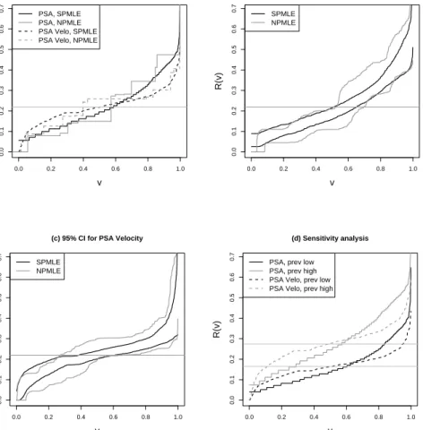
We compare PSA and PSA velocity as risk prediction markers for prostate cancer utilizing the predictiveness curve technique. A logistic regression risk model with a Box-Cox transformation of the marker is employed. The two semiparametric estimators of the predictiveness curves are fairly similar to each other for both PSA and PSA velocity and are much smoother than the nonparametric ones. The semiparametric maximum likelihood and nonparametric estimators are displayed in Figure 1(a). PSA has more steep predictiveness curves, suggesting that it is a better marker for predicting risk of prostate cancer.
The pointwise 95% percentile bootstrap confidence intervals forR(v) constructed from semi-parametric maximum likelihood estimators are displayed in Figure 1(b)(c), with variability in ˆ
ρ incorporated. They are much narrower compared to those constructed from nonparametric
estimators.
Table 4(a) presents results comparing PSA and PSA velocity with respect to risk percentiles,
R(v), for v = 10% and 90%, and risk stratum sizes, R−1(p), for a low risk threshold 10% and
a high risk threshold 30%. P-values for comparing markers are based on bootstrap variance estimates. Using the semiparametric methods we conclude that PSA is a significantly better risk prediction marker than PSA velocity. Specifically, it is better for predicting high risk (larger
R(0.9)), better for predicting low risk (smallerR(0.1)), and it classifies more people into the low and high risk ranges. In contrast, these conclusions cannot be drawn with the nonparametric methods due to their large sampling variability.
In practice, there may not always be a cohort for estimating prevalence. Oftentimes an investigator plugs in a specific prevalence value and treats it as known. We illustrate application of a sensitivity analysis using our example. We studyρ= 0.165 andρ= 0.274 which correspond to a 25% change in ˆρ= 0.219. The corresponding predictiveness curves are displayed in Figure 1(d). Note that the comparison of predictiveness curves with respect to steepness is not sensitive to perturbation in prevalence. PSA appears overall to be a better risk prediction marker than PSA velocity in the sense that the risk percentiles vary more. Comparison at particular risk thresholds, on the other hand, are affected by prevalence. For example, whenρ= 0.165, based on
0.0 0.2 0.4 0.6 0.8 1.0 0.0 0.1 0.2 0.3 0.4 0.5 0.6 0.7
(a) Predictiveness Curves
v
R(v)
PSA, SPMLE PSA, NPMLE PSA Velo, SPMLE PSA Velo, NPMLE
0.0 0.2 0.4 0.6 0.8 1.0 0.0 0.1 0.2 0.3 0.4 0.5 0.6 0.7 (b) 95% CI for PSA v R(v) SPMLE NPMLE 0.0 0.2 0.4 0.6 0.8 1.0 0.0 0.1 0.2 0.3 0.4 0.5 0.6 0.7
(c) 95% CI for PSA Velocity
v R(v) SPMLE NPMLE 0.0 0.2 0.4 0.6 0.8 1.0 0.0 0.1 0.2 0.3 0.4 0.5 0.6 0.7 (d) Sensitivity analysis v R(v)
PSA, prev low PSA, prev high PSA Velo, prev low PSA Velo, prev high
Figure 1. (a) The predictiveness curves for PSA and PSA velocity for predicting prostate
cancer;(b)(c) their 95% pointwise confidence intervals constructed from percentiles of the boot-strap distribution; and (d) sensitivity analysis. The horizontal lines indicate disease prevalences plugged in. SPMLE: semiparametric maximum likelihood estimator; NPMLE: nonparametric maximum likelihood estimator.
Table 4
Comparisons between (a) PSA and PSA velocity and (b) between PSA and PSA plus other risk factors for predicting risk of prostate cancer.
(a)
Measure Method PSA PSA Velocity pvalue Est 95% CI Est 95% CI R(0.1) NPMLEa 0.079 (0.043,0.110) 0.088 (0.044, 0.131) 0.730 SPMLEb 0.072 (0.046, 0.109) 0.122 (0.075, 0.159) 0.027 R(0.9) NPMLE 0.474 (0.369, 0.577) 0.302 (0.253, 0.402) 0.005 SPMLE 0.413 (0.356, 0.476) 0.313 (0.275, 0.356) <0.001 R−1(0.1) NPMLE 0.304 (0.050, 0.39) 0.155 (0.019, 0.305) 0.178 SPMLE 0.188 (0.073, 0.291) 0.06 (0.020, 0.142) 0.021 1−R−1(0.3) NPMLE 0.302 (0.140, 0.447) 0.168 (0.007, 0.501) 0.274 SPMLE 0.244 (0.191, 0.296) 0.129 (0.030, 0.197) 0.009 R−1(0.3)−R−1(0.1) NPMLE 0.393 (0.210, 0.664) 0.677 (0.301, 0.933) 0.100 SPMLE 0.568 (0.443, 0.724) 0.811 (0.668, 0.935) 0.004 (b)
Measure Method PSA PSA + other factors pvalue Est 95% CI Est 95% CI R(0.1) SPMLE 0.072 (0.045, 0.109) 0.070 (0.039, 0.094) 0.798 R(0.9) SPMLE 0.413 (0.356, 0.476) 0.429 (0.372, 0.502) 0.223 R−1(0.1) SPMLE 0.188 (0.073, 0.291) 0.204 (0.109, 0.310) 0.595 1−R−1(0.3) SPMLE 0.244 (0.191, 0.296) 0.243 (0.203, 0.281) 0.952 R−1(0.3)−R−1(0.1) SPMLE 0.568 (0.443, 0.724) 0.554 (0.436, 0.662) 0.667
a: nonparametric maximum likelihood estimator b: semiparametric maximum likelihood estimator
the semipmarametric maximum likelihood procedure, PSA assigns significantly more people into low risk range than PSA velocity, with estimates ofR−1(0.1) being 31.3% and 13.5% respectively (p-value< 0.001). PSA is also a significantly better marker for predicting high risk than PSA velocity, with estimates of 1−R−1(0.3) being 12.5% and 2.9% respectively (p-value<0.001). In contrast, whenρ= 0.263, estimates ofR−1(0.1) become 9.7% and 3.8% for PSA and PSA velocity, and estimates of 1−R−1(0.3) are 38.9% and 36.9% respectively. None of the comparisons are significant (p-value=0.192 and 0.736). The comparison with respect to percentage classified into the equivocal risk range is significant when ρ= 0.165 (p-value<0.001) but not when ρ= 0.274 (p-value=0.375).
7. Extension of Semiparametric Estimation
The semiparametric estimators can be extended naturally to accommodate multiple predictors or to settings where the monotone increasing risk assumption is not true. LetFR, FDR, FDR¯
populations respectively. We first calculateRisk(Yi) as the predicted risk for subjectibased on
a a standard logistic regression model with offset log{(1−ρˆ)/ρˆ). Then estimateFR according to
ˆ
ρFDR+ (1−ρˆ)FDR¯ . Note thatFDR and FDR¯ can be estimated “empirically” using
˜ FDR(p) = 1 nD nD X i=1 I n [ Risk(YDi)≤p o , ˜ FDR¯ (p) = 1 nD¯ nD¯ X i=1 I n [ Risk(YDi¯ )≤p o ,
or based on the semiparametric maximum likelihood method
ˆ FDR(p) = 1 n n X i=1 c LRR n [ Risk(Yi) o InRisk[(Yi)≤p o nD¯ n + nD n LcRR n [ Risk(Yi) o , ˆ FDR¯ (p) = 1 n n X i=1 I n [ Risk(Yi)≤p o nD¯ n + nD n LcRR n [ Risk(Yi) o, whereLcRR n [ Risk(Yi) o =Risk[(Yi)/ n 1−Risk[(Yi) o
×(1−ρˆ)/ρˆ. Compute semiparametric max-imum likelihood estimators ˆR(v) = ˆFR−1(v) and ˆR−1(p) = ˆFR(p) and semiparametric “empirical”
estimators ˜R(v) = ˜FR(p) and ˜R−1(p) = ˜FR(p). Following similar arguments as in the single
marker setting, asymptotic distribution theory presented in Theorems 7 and 8 can be derived. In practice, since estimation of asymptotic variance involves both numerical differentiation and nonparametric density estimation, we rely on resampling techniques for inference.
Theorem 7
Asn→ ∞, √nnRˆ−1(p)−R−1(p)oconverges to a normal random variable with mean zero
and variance Σ2M.R(p) = var √ nQM(p)−R−1(p) + ∂R−1(p) ∂θ T var n√ n( ˆθ−θ) o ∂R−1(p) ∂θ + 2 ∂R−1(p) ∂θ T cov h√ n ˆ θ−θ ,√nQM(p)−R−1(p) i ,
and √nnRˆ(v)−R(v)oconverges to a normal random variable with mean zero and variance Σ1M.R(v) = ∂R(v) ∂v 2 Σ2M.R{R(v)}, where QM(p) =ρ 1 n n X i=1 c LRR n [ Risk(Yi) o I{Risk(Yi)≤p} nD¯ n + nD n LcRR n [ Risk(Yi) o + (1−ρ)1 n n X i=1 I{Risk(Yi)≤p} nD¯ n + nD n LcRR n [ Risk(Yi) o. Theorem 8
Asn→ ∞, √nnR˜−1(p)−R−1(p)oconverges to a normal random variable with mean zero and variance Σ2E.R(p) = var √ nQE(p)−R−1(p) + ∂R−1(p) ∂θ T var n√ n( ˆθ−θ) o ∂R−1 (p) ∂θ + 2 ∂R−1(p) ∂θ T covh√nθˆ−θ,√nQE(p)−R−1(p) i , and √n n ˆ R(v)−R(v) o
converges to a normal random variable with mean zero and variance
Σ1E.R(v) = ∂R(v) ∂v 2 Σ2E.R{R(v)}, where QE(p) =ρ 1 nD nD X i=1 I{Risk(YDi) ≤p}+ (1−ρ) 1 nD¯ nD¯ X i=1 I{Risk(YDi¯ )≤p}.
Components of these asymptotic variance terms can be calculated similar to those in the single marker setting by replacing the marker distribution with the risk distribution. Note that when Y has only one component and under the monotone increasing risk assumption, the variance
expressions in Theorems 7 and 8 reduce to those in Theorems 1-4, i.e. QM(p) = ˆF{G−1(p)}and
QE(p) = ˜F{G−1(p)}.
7.1 Illustration
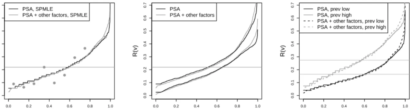
We illustrate using the simulated case-control sample described in Section 6. We compare the logistic risk model based on PSA alone with a more comprehensive risk model that combines Box-Cox transformation of PSA and other risk factors, including family history of prostate cancer, DRE, and previous negative biopsies. All of these factors are highly statistically significant (Thompson et al., 2006).
Figure 2(a) displays the semiparametric maximum likelihood estimators of the predictiveness curves for PSA alone and for PSA plus other factors (the semiparametric “empirical” estimators are similar), for ˆρ = 21.9%. The two risk models have very similar predictiveness curves. To assess model fit, we let Risk[(Y) be risk estimates from the model employing PSA and other risk factors and partition the observations into deciles of the distribution for Risk[(Y). For
k ∈ {1, . . . ,10}, we estimate ˆP(D = 1|k, S) as the observed proportion of cases within the kth
group. The population risk within thekth group,P(D= 1|k) is estimated according to ˆ P(D= 1|k) 1−Pˆ(D= 1|k) = ˆ P(D= 1|k, S) 1−Pˆ(D= 1|k, S) nD¯ nD 1−ρˆ ˆ ρ .
At the midpoints of thekthgroup, a visual comparison can be made between these points and the predictiveness curve by superimposing the value of ˆP(D= 1|k) on the plot. This comparison of observed risk and average risk within deciles of modeled risk is the basis for the Hosmer-Lemeshow test (Hosmer and Lemeshow, 1980). Our approach provides a graphical display that generalizes to case-control data. In Figure 2(a), there seems to be a slight lack of fit in the middle of the curve but good fit at both ends which are the regions of primary interest. Confidence intervals for R(v) constructed with the semiparametric maximum likelihood estimators are presented in Figure 2(b). Variabilities from the two risk models appear to be similar in magnitude.
Detailed results comparing the two models for predictiveness are shown in Table 4(b). Briefly, the percentages of people classified into the low, high, or equivocal risk ranges are not significantly
0.0 0.2 0.4 0.6 0.8 1.0 0.0 0.1 0.2 0.3 0.4 0.5 0.6 0.7
(a) Predictiveness Curves
v
R(v)
PSA, SPMLE
PSA + other factors, SPMLE
0.0 0.2 0.4 0.6 0.8 1.0 0.0 0.1 0.2 0.3 0.4 0.5 0.6 0.7 (b) 95% SPMLE CI v R(v) PSA
PSA + other factors
0.0 0.2 0.4 0.6 0.8 1.0 0.0 0.1 0.2 0.3 0.4 0.5 0.6 0.7 (c) Sensitivity analysis v R(v)
PSA, prev low PSA, prev high
PSA + other factors, prev low PSA + other factors, prev high
Figure 2. (a) The semiparametric predictiveness curves for PSA and PSA plus other factors
for predicting risk prostate cancer,the dots are average risk within deciles of modeled risk based on the latter model; (b) their 95% pointwise confidence intervals using percentiles of the boot-strap distribution; and (c) sensitivity analysis. The horizontal lines indicate disease prevalences. SPMLE: semiparametric maximum likelihood estimator; NPMLE: nonparametric maximum like-lihood estimator.
different between the two models, nor are the 10th and 90th percentiles of risk. Thus including other factors in the model in addition to PSA does not lead to a significant improvement in risk stratification even when these factors are all statistically significant in the multivariate logistic regression model. It reinforces our earlier argument that the risk model by itself is not enough to characterize the population performance of a risk prediction model.
Again, we conducted sensitivity analysis with fixedρ= 0.165 andρ= 0.274, the correspond-ing predictiveness curves are displayed in Figure 2(c). Different choices of ρ do not change our conclusion about the comparison between the two risk models.
8. Concluding Remarks
In this article we have developed flexible semiparametric and nonparametric estimators of the predictiveness curve for case-control studies. This is particularly valuable for evaluating a risk prediction marker or model early in its development when case-control designs are most com-mon. Both estimators are easy to compute: risk models can be estimated utilizing standard statistical procedures, and risk distributions can be calculated easily based on analytic formulae. The nonparametric estimator is highly robust but demands very large sample sizes for reasonable precision. This begs for introduction of smoothing techniques in future research. The
semipara-metric estimators, in contrast, have satisfactory finite-sample performance. Another approach to estimate the predictiveness curve is based on its relationship with the ROC curve. This is currently under investigation (Huang and Pepe, 2007).
In terms of comparison between the two semiparametric estimators, their validity both rely upon assumptions about the risk model. If the risk model is misspecified, bias can be introduced into both estimators. This, however, may not be a big concern since the risk model can be made highly flexible using techniques such as regression splines. Given a well specified model, the semi-parametric maximum likelihood estimator is more efficient than the its “empirical” counterpart. Asymptotic relative efficiency of the former versus the latter is a complicated function of the disease prevalence, separation between cases and controls, case-control sampling ratio, and the quantile of interest. In the examples, we showed that when the disease prevalence is medium, the two estimators have similar efficiency. We note that for rare diseases, using the model-based approach may achieve considerable efficiency gains compared to the “empirical” approach for certain quantiles (Huang, 2007).
An important use of the asymptotic theory is to guide study design. To design an efficient case-control study for evaluating a risk model, the optimal case-control sampling ratio is dictated by the disease prevalence, separation between cases and controls, and the measure that are of primary interest. A detailed study can be found in Huang (2007).
Comparing markers or models for their risk stratification capacity is of great significance in medical practice. Researchers are often interested in whether additional risk factors which may be hard to measure can lead to a significant improvement in utility compared to an existing model. More research on methods to evaluate incremental value is warranted. Methods described here might be adapted for such purposes. An important issue pertaining to the general risk model methods is overfitting when the number of predictors gets large relative to the sample size. The effectiveness of cross-validation techniques for addressing biases needs to be investigated.
Pepe et al. (2008a) proposed displaying the predictiveness curve and curves displaying true and false positive rates together for maximum information. Specifically, to evaluate a risk pre-diction marker, one will be interested in knowing not only 1−R−1(p), the proportion of the
population with risk above p, but also the proportion of diseased subjects correctly classified (the true positive rate TPR(p) = P(Risk(Y) > p|D= 1) ) and the proportion of non-diseased subjects incorrectly classified (the false positive rate FPR(p) =P(Risk(Y)> p|D= 0)), accord-ing to the classification rule ‘Risk(Y)> p’. Our semiparametric and nonparametric procedures developed in this manuscript yield estimators of FD, FD¯ and F as by-products, which can be
directly plugged into TPR(p) =FD{F−1(p)}and FPR(p) =FD¯{F−1(p)}for estimation of these
quantities. Asymptotic theory for corresponding semiparametric estimators can be developed in a similar fashion.
Acknowledgments
The authors are grateful for support provided by NIH grants GM-54438 and NCI grants CA86368.
References
Anderson, J. A. (1972). Separate sample logistic discrimination.Biometrika 59(1), 19-35.
Anderson, K.M. and Odell, P.M. and Wilson, P.W. and Kannel, W.B. (1991). Cardiovascular disease risk profiles.American Heart Journal 121, 293-298.
Baker, S. G., Kramer, B. S., and Srivastava, S. (2002). Markers for early detection of cancer: Statistical guidelines for nested case-control studies.BMI Medical Research Methodology,2:4. Barlow, R. E. and Bartholomew, D. J. and Bremner, J. M. and Brunk, H. D. (1972).
Statisti-cal Inference Under Order Restrictions: The Theory and Application of Isotonic Regression.
Wiley, London.
Bickel, P. J. and Klaassen, C. A. J. and Ritov, Y. and Wellner, J. A. (2002). Efficient and
Adaptive Estimation for Semiparametric Models. Springer.
Billingsley, P. (1999).Convergence of Probability Measures. Wiley, New York.
Breslow, N. E. and Robins, J. M. and Wellner, J. A. (2000). On the semi-parametric efficiency of logistic regression under case-control sampling.Bernoulli 6(3),447-455.
Bura, E. and Gastwirth, J. L. (2001). The binary regression quantile plot: assessing the impor-tance of predictors in binary regression visually.Biometrical Journal 43 (1), 5-21.
Cole, T. J. and Green, P. J. (1992). Smoothing reference centile curves: The LMS method and penalized likelihood.Statistics in Medicine 11(165),1305-1319.
Cook, N. R. (2007). Use and misuse of the receiver operating characteristic curve in risk predic-tion.Circulation 115,928-935.
Gail, M.H. and Brinton, L.A. and Byar, D.P. and Corle, D.K. and Green, S.B. and Schairer, C. and Mulvihill, J.J. (1989). Projecting individualized probabilities of developing breast cancer for white females who are being examined annually . JNCI 81(24), 1879-1886.
Gail, M. H. and Pfeiffer, R. M. (2005). On criteria for evaluating models of absolute risk.
Bio-statistics 6(2),227-239.
Gilbert, P. B. (2000). Large sample theory of maximum likelihood estimates in semiparametric biased sampling models.Annals of Statistics 28(1),151-194.
Gilbert, P. B. and Lele, S. and Vardi, Y. (1999). Maximum likelihood estimation in semipara-metric selection bias models with application to AIDS vaccine trials.Biometrika 86, 27-43. Gill, R. D. and Vardi, Y. and Wellner, J. A. (1988). Large sample theory of empirical distributions
in biased sampling models.Annals of Statistics 16,1069-1112.
Green, D. M. and Swets, J. A. (1966). Signal detection theory and psychophysics. Wiley, New York.
Hosmer, D.W. and Lemesbow, S. (1980). Goodness of fit tests for the multiple logistic regression model.Communications in Statistics-Theory and Methods 9(10), 1043-1069.
Huang, Y. (2007). Evaluating the predictiveness of continuous biomarkers.UW thesis.
Huang, Y. and Pepe, M. S. and Feng, Z. (2007). Evaluating the predictiveness of a continuous marker.Biometrics 63(4), 1181-1188.
Huang, Y. and Pepe, M. S. (2007). A parametric ROC model based approach for evaluating the predictiveness of continuous markers in case-control studies.UW Biostatistics Working Paper
Series 318.
Huang, Y. and Pepe, M. S. (2008). Semiparametric and nonparametric methods for evaluating risk prediction markers in case-control studies. UW Biostatistics Working Paper Series 318. Lloyd, C. J. (2000). Maximum likelihood estimation of misclassification rates of a binomial
re-gression.Biometrika 87(3), 700-705.
Lloyd, C. J. (2002). Estimation of a Convex ROC Curve. Statistics & Probability Letters 59,
99-111.
Pencina, M.J. and D’Agostino Sr., R.B. and D’Agostino Jr., R.B. and Vasan, R.S. (2007). Eval-uating the added predictive ability of a new marker: From area under the ROC curve to reclassification and beyond.Statistics in Medicine (In Press).
Pepe, M. S. (2000). An interpretation for the ROC curve and inference using GLM procedures.
Biometrics 56,352-359.
Pepe, M. S. (2003).The Statistical Evaluation of Medical Tests for Classification and Prediction. Oxford University Press.
Pepe, M. S. and Etzioni, R. and Feng, Z. and Potter, J. D. and Thompson, M. L. and Thornquist, M. and Winget, M. and Yasui, Y. (2001) Phases of biomarker development for early detection of cancer. Journal of the National Cancer Institute 93(14), 1054-1061.
Pepe, M. S. and Feng, Z. and Huang, Y. and Longton, G. M. and Prentice, R. and Thompson, I. M. and Zheng, Y. (2008a). Integrating the predictiveness of a marker with its performance as a classifier.American Journal of Epidemiology 167(3), 362-368.
Pepe, M. S. and Feng, Z. and Janes, H. and Bossuyt, P. M. and Potter, J. D. (2008b). Pivotal evaluation of the accuracy of a classification biomarker: the PRoBE study design.Journal of
Prentice, R. L. and Pyke, R. (1979). Logistic Disease Incidence Models and Case-Control Studies.
Biometrika 66(3),403-411.
Qin, J. and Lawless, J. (1994). Empirical likelihood and general estimating equations.The Annals
of Statistics 22(1),300-325.
Qin, J. and Zhang, J. (1997). A goodness-of-fit test for logistic regression models based on case-control data.Biometrika 84(3),609-618.
Qin, J. and Zhang, J. (2003). Using logistic regression procedures for estimating receiver operating characteristic curves.Biometrika 93(3), 585-596.
Ransohoff, D. F. (2007). How to improve reliability and efficiency of research about molecular markers: roles of phases, guidelines, and study design. Journal of Clinical Epidemiology 60,
1205-1219.
Simon, R. (2005). Roadmap for developing and validating therapeutically relevant genomic clas-sifiers.Journal of Clinical Oncology 23(29), 7332-7341.
Thompson, I. M. and Pauler Ankerst, D. and Chi, C. (2006). Assessing prostate cancer risk: results from the prostate cancer prevention trial. Journal of the National Cancer Institute 98, 529-534.
van der Vaart, A. W. (1998).Asymptotic Statistics. Cambridge University Press.
Vardi, Y. (1985). Empirical distributions in selection bias models. Annals of Statistics 13, 178-203.
Zhang, B. (2000). Quantile estimation under a two-sample semi-parametric model. Bernoulli
9. Appendix
9.1 Components for Asymptotic Variances of Semiparametric Estimators in Theorems 1-4
Consider ˆρ estimated from a cohort independent of the case-control sample, or the parent cohort where the case-control sampled is nested within. Assume the size of the cohort isλtimes the size of the case-control sample. Denote
ˆ F?(t) = ρFˆD(t) + (1−ρ) ˆFD¯(t) ˜ F?(t) = ρF˜D(t) + (1−ρ) ˜FD¯(t), ˆ θ? = ˆ θ0S+ log nD¯ nD ρ 1−ρ ˆ θ1S ,
then the following Lemma holds.
Lemma 0 varh√nnFˆ(t)−F(t)oi={FD(t)−FD¯(t)}2ρ(1−ρ)/λ+ var h√ nnFˆ?(t)−F(t)oi, var h√ n n ˜ F(t)−F(t) oi ={FD(t)−FD¯(t)}2ρ(1−ρ)/λ+ var h√ n n ˜ F?(t)−F(t) oi , var n√ n ˆ θ−θ o = 1 λρ(1−ρ) 0 0 0 + var n√ n ˆ θ?−θ o covh√nθˆ−θ,√nnFˆ(t)−F(t)oi= FD(t)−FD¯(t) λ + cov h√ nθˆ?−θ,√nnFˆ?(t)−F(t)oi. Suppose logit{G(θ, Y)}=θ0+θT1r(Y) =α+ log ρ 1−ρ +βTr(Y).
Let ˆα, ˆβ be the MLE of α, β based on the semiparametric likelihood (3). Let η = nD/nD¯.
The following Lemmas are needed to calculate the asymptotic variances of the semiparametric predictiveness curve estimators. Lemma 1 characterizes the distribution of ˆθ?, a result proved in Prentice and Pyke (1979), Qin and Zhang (1997) and Zhang (2000). Lemmas 2 to 7 present
asymptotic theory for ˆF?, ˜F? and the correlation between them and ˆθ?. Proofs of Lemmas 2-7 are given in Appendix B.
Lemma 1 Let A0(t) = Z t −∞ expα+βTr(y) 1 +ηexp{α+βTr(y)}dFD¯(y), A1(t) = Z t −∞ r(y) expα+βTr(y) 1 +ηexp{α+βTr(y)}dFD¯(y), A2(t) = Z t −∞ r(y)r(y)Texpα+βTr(y) 1 +ηexp{α+βTr(y)} dFD¯(y), A(t) = A0(t) A1(t) T A1(t) A2 , and A=A(∞). IfA−1 exists, √ n αˆ −α ˆ β−β →d N(0,Σ), where Σ = 1 +η η A −1− 1 +η 0 0 0 . Lemma 2 Asn→ ∞,√n n ˆ F?(t)−F(t) o
converges weakly in D[−∞,∞] to W(t), a Gaussian process with mean 0 and covariance function specified by
E{WM(s)WM(t)} = (1−ρ)2(1 +η){FD¯(s∧t)−FD¯(s)FD¯(t)}+ρ2 1 +η η {FD(s∧t)−FD(s)FD(t)} − 1 +η η {ρ−(1−ρ)η}2 A0(s∧t)− A0(s), A1(s)T A−1 A0(t) A1(t) . Lemma 3 √ n ˆ F?−1(v)−F−1(v) d →W{F−1(v)}/f{F−1(v)}
onD[a, b], where W is the Gaussian process with continuous sample path as specified in Lemma 2. Lemma 4Asn→ ∞,√n n ˜ F?(t)−F(t) o
converges weakly inD[−∞,∞] toWE(t), a Gaussian
process with mean 0 and covariance function specified by
E{WE(s)WE(t)} = (1−ρ)2(1 +η){FD¯(s∧t)−FD¯(s)FD¯(t)}+ρ2 1 +η η {FD(s∧t)−FD(s)FD(t)}. Lemma 5 √ nF˜?−1(v)−F−1(v)→d WE{F−1(v)}/f{F−1(v)}
onD[a, b], whereWE is the Gaussian process with continuous sample path as specified in Lemma
Lemma 6 cov √n αˆ −α ˆ β−β ,√nnFˆ?(t)−F(t)o = cov √n αˆ −α ˆ β−β ,√nnF˜?(t)−F(t)o = 1 +η η {ρ−η(1−ρ)}A−1 A0(t) A1(t) − ρFD(t) −η(1−ρ)FD¯(t) 0 +op(1) Lemma 7 cov √n αˆ −α ˆ β−β ,√n n ˆ F?−1(v)−F−1(v) o = cov √n αˆ −α ˆ β−β ,√n n ˜ F?−1(v)−F−1(v) o = 1 f{F−1(v)} 1 +η η {ρ−η(1−ρ)}A −1 A0 F−1(v) A1 F−1(v) − 1 +η η ρFD{F −1(v)} −η(1−ρ)F ¯ D{F−1(v)} 0 +op(1)
9.2 Proofs of Lemmas and Theorems for Semiparametric Estimators
9.2.1 Proof of Lemma 0 √ nnFˆ(t)−F(t)o = √n n ˆ F(t)−F?(t) o +√n n ˆ F?(t)−F(t) o ' √n{ρFˆ D(t) + (1−ρˆ)FD¯(t)−F(t)}+ √ n n ˆ F?(t)−F(t) o . (5)