Dynamic Travel Time Maps

(1)

Dynamic Travel Time Maps

Sotiris Brakatsoulas

Dieter Pfoser

RA Computer Technology Institute

Akteou 11

GR-11851 Athens, Greece

Nectaria Tryfona

Talent SA

Karytsi Sq. 4

GR-11851 Athens, Greece

Agn`es Voisard

Fraunhofer ISST

Mollstr. 1

D-10178 Berlin, Germany

SYNONYMS

spatiotemporal data warehousing; travel time computation

DEFINITION

The application domain of intelligent transportation is plagued by a shortage of data sources that adequately assess traffic situations. Currently, to provide routing and navigation solutions an unreliable travel time database that consists of static weights as derived from road categories and speed limits is used for road networks. With the advent of Floating Car Data (FCD) and specifically the GPS-based tracking data component, a means was found to derive accurate and up-to-date travel times, i.e., qualitative traffic information. FCD is a by-product in fleet management applications and given a minimum number and uniform distribution of vehicles, this data can be used for accurate traffic assessment and also prediction. Map-matching the tracking data produces travel time data related to a specific edge in the road network. TheDynamic Travel Time Map (DTTM) is introduced as a means to efficiently supply dynamic weights that are derived from a collection of historic travel times. The DTTM is realized as a spatiotemporal data warehouse.

HISTORICAL BACKGROUND

Dynamic Travel Time Maps were introduced as an efficient means to store large collections of travel time data as produced by GPS tracking of vehicles [6]. DTTMs can be realized using standard data warehousing technology available in most commercial database products.

SCIENTIFIC FUNDAMENTALS

A major accuracy problem in routing solutions exists due to the unreliable travel time associated with the underlying road network.

A road network is modeled as a directed graphG= (V, E), whose verticesV represent intersections between links and edgesE represent links. Additionally, a real-valued weight function w:E →R _{is given, mapping edges to}

weights. In the routing context, such weights typically correspond to speed types derived from road categories or based on average speed measurements. However, what is important is that such weights are static, i.e., once defined they are rarely changed. Besides, such changes are rather costly as the size of the underlying database is in the order of dozens of Gigabytes.

Although the various algorithmic solutions for routing and navigation problems [7, 3] are still subject to further research, the basic place for improving solutions to routing problems is this underlying weight-based database

(2)

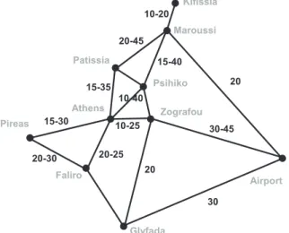
The DTTM will be a means to make the weight database fully dynamic with respect to not only a spatial (what road portion) but also a temporal argument (what time of day). The idea is to derive dynamic weights from collectedfloating car data (FCD). Travel times and thus dynamic weights are derived from FCD by relating its tracking data component to the road network using map-matching algorithms[1]. Using the causality between historic and current traffic conditions, weights - defined based on temporal parameters - will replace static weights and will induce impedance in traversing some links. Figure 1 gives an example of fluctuating travel times in a road network. Glyfada Airport Faliro Pireas Athens _Zografou Psihiko Patissia Maroussi Kifissia 20 30-45 20 10-20 10-25 20-25 20-30 15-30 10-40 30 15-35 20-45 15-40

Figure 1: Fluctuating travel times (in minutes) in a road network example (Athens, Greece)

Travel Time Causality in the Road Network The collection of historical travel time data provides a strong basis for the derivation of dynamic weights provided that one can establish the causality of travel time with respect to time (time of the day) and space (portion of the road network)[1, 2].

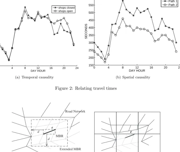
Temporal causality establishes that for a given path, although the travel time varies with time, it exhibits a reoccurring behavior. An example of temporal causality is shown in Figure 2(a). For the same path, two travel time profiles, i.e., the travel time varying with the time of the day, are recorded for different weekdays. Although similar during nighttime and most daytime hours, the travel times differ significantly during the period of 16h to 22h. Here, on one of the days the shops surrounding this specific path were open from 17h to 21h in the afternoon.

Spatial causality establishes that travel times of different edges are similar over time. An example is given in Figure 2(b). Given two different paths, their travel time profiles are similar. Being in the same shopping area, their travel time profile is governed by the same traffic pattners, e.g., increased traffic frequency and thus increased travel times from 6h to 20h, with peaks at 8h and around noon.

Overall, discovering such temporal and spatial causality, affords hypothesis testing and data mining on historic data sets. The outcome is a set of rules that relate (cluster) travel times based on parts of the road network and the time in question. A valid hypothesis is needed that selects historic travel time values to compute meaningful weights.

Characteristic Travel Times = Aggregating Travel Times A problem observed in the example of Figure 2(b) is that travel times, even if causality is established, are not readily comparable. Instead of considering absolute travel times that relate to specific distances, the notion of relative travel timeρis introduced, which for edgeeis defined as follows,

(1) ρ(e) = τ(e)

l(e)

(3)

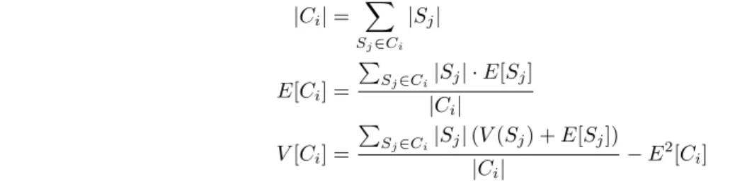
Given a set of relative travel times P(e) related to a specific network edgee and assuming that these times are piecewise independent, the characteristic travel time χ(P) is defined by the triplet cardinality, statistical mean, and variation as follows,

χ(P) = {|P|, E[P], V[P]} (2) E[P] = X ρ∈P ρ |P| (3) V[P] = X ρ∈P (ρ−E[P])2 |P| (4)

The critical aspect for the computation ofP(e) is the set of relative travel times selected for the edgeein question based on temporal and spatial inclusion criteriaIT(e) andIS(e), respectively.

(5) P(e) ={ρ(e∗

, t) :e∗

∈IS(e)∧t∈IT(e)}

IS(e), a set of edges, contains typically the edge e itself but can be enlarged as we will see later on to include

further edges as established by an existing spatial causality between the respective edges. IT(e), a set of time

periods, is derived by existing temporal causality. The characteristic travel time essentially represents a dynamic weight, since depending on a temporal inclusion criterion (e.g., time of the day, day of the week, month, etc.), its value varies.

FCD and thus travel times are not uniformly distributed over the entire road network, e.g., taxis prefer certain routes through the city. To provide a dynamic weight database for the entire road network, a considerable amount of FCD is needed on a per edge basis, i.e., the more available data, the more reliable will be the characteristic travel time.

While it is possible to compute the characteristic travel times for frequently traversed edges only based on data related to the edge in question, for the non-frequently traversed edges, with their typical lack of data, complementary methods are needed. The simplest approach is to substitute travel times by static link-based speed types as supplied by map vendors. However, following the spatial causality principle, the following three prototypical methods can be defined. The various approaches differ in terms of the chosen spatial inclusion criterionIS(e), with each method supplying its own approach.

Simple Method. Only the travel times collected for a specific edge are considered. IS(e) ={e}.

Neighborhood Method. Exploiting spatial causality, i.e., the same traffic situations affecting an entire area, we use a simple neighborhood approach by considering travel times of edges that are (i) contained in an enlarged minimum bounding rectangle (MBR) around the edge in question and (ii) belong to the same road category. Figure 3(a) shows a network edge (bold line) and an enclosing MBR (small dashed rectangle) that is enlarged by a distancedto cover the set of edges considered for travel time computation (thicker gray lines). IS(e) ={e∗:e∗

contained in d-expanded MBR(e)∧L(e∗_{) =}

L(e)}, with L(e) being a function that returns the road category of edgee.

Tiling Method. Generalizing the neighborhood method, a fixed tiling approach for the network is used to categorize edges into neighborhoods. It effectively subdivides the space occupied by the road network into equal sized tiles. All travel times of edges belonging to the same tile and road category as the edge in question are used for the computation of the characteristic travel time. Figure 3(b) shows a road network and a grid. For the edge in question (bold line) all edges belonging to the same tile (thicker gray lines) are used for the characteristic travel time computation. IS(e) ={e∗:e∗∈T ile(e)∧L(e∗) =L(e)}

Both, the Neighborhood and the Tiling Method, are effective means to compensate for missing data when computing characteristic travel times. Increasing the d in the Neighborhood Method, increases the number of edges and thus the potential number of relative travel times considered. To achieve this with the Tiling Method, the tile sizes have to be increased.

Dynamic Travel Time Map The basic requirement to the DTTM is the efficient retrieval of characteristic travel times, and, thus, dynamic weights on a per-edge basis. Based on the choice of the various travel time computation methods, the DTTM needs to support each method in kind.

(4)

The travel time computation methods use arbitrary temporal and spatial inclusion criteria. This suggests the use of a data warehouse with relative travel times as a data warehouse fact and space and time as the respective dimensions. Further, since the tiling method proposes regular subdivisions of space, one has to account for a potential lack of travel time data in a tile by considering several subdivisions of varying sizes.

The multidimensional data model of the data warehouse implementing the DTTM is based on a star schema. Figure 4 shows the schema comprising five fact tables and two data warehouse dimensions. The two data warehouse dimensions relate to time, TIME DIM, and to space, LOC DIM, implementing the respective granularities as described in the following.

Spatial subdivisions of varying size can be seen as subdivisions of varying granularity that form a dimensional hierarchy. This subdivisions relate to the Tiling Method used for characteristic travel time computation. A simple

spatial hierarchy with quadratic tiles of side length 200, 400, 800, and 1600 meters respectively is adopted, i.e., four tiles ofxm side length are contained in the corresponding greater tile of 2xm side length. Consequently, the spatial dimension is structured according to the hierarchyedge, area 200, area 400,area 800,area 1600. Should little travel time data be available at one level in the hierarchy, one can consider a higher level, e.g., area 400 instead of area 200.

Obtaining characteristics travel times means to relate individual travel times. Using an underlying temporal granularity of one hour, all relative travel times that were recorded for a specific edge during the same hour are assigned the same timestamp. The temporal dimension is structured according to a simple hierarchy formed by thehour of the day, 1 to 24, with, e.g., 1 representing the time from 0am to 1am, theday of the week, 1 (Monday) to 7(Sunday),week, the calendar week, 1 to 52,month, 1 (January) to 12 (December), andyear, 2000 - 2003, the years for which tracking data was available to us.

The measure that is stored in the fact tablesis the characteristic travel timeχ in terms of the triplet

{|P|, E[P], V[P]}. The fact tables comprise a base fact table EDGE TT and four derived fact tables,

AREA 200 TT, AREA 400 TT, AREA 800 TT, and AREA 1600 TT, which are aggregations of EDGE TT implementing the spatial dimension hierarchy. Essentially, the derived fact tables contain the characteristic travel time as computed by the Tiling Method for the various extents.

In aggregating travel times along the spatial and temporal dimensions, the characteristic travel time χ(C) =

{|Ci|, E[Ci], V[Ci]} for a given level of summarization can be computed based on the respective characteristic

travel times of a lower level,χ(Sj), without using the initial set of characteristic travel timesP as follows.

|Ci|= X Sj∈Ci |Sj| (6) E[Ci] = P Sj∈Ci|Sj| ·E[Sj] |Ci| (7) V[Ci] = P Sj∈Ci|Sj|(V(Sj) +E[Sj]) |Ci| −E2_[_C i] (8)

Implementation and Empirical Evaluation To evaluate its performance, the DTTM was implemented using an Oracle 9i installation and following the data warehouse design “best practices” described in [5, 8]. The primary goal of these best practices is to successfully achieve the adoption of the “star transformation” query processing scheme by the Oracle optimizer. The latter is a special query processing technique, which gives fast response times when querying a star schema.

The steps involved in achieving an optimal execution plan for a star schema query require the setup of an efficient indexing scheme and some data warehouse-specific tuning of the database (proper setting of database initialization parameters and statistics gathering for use by the cost-based optimizer of Oracle). The indexing scheme is based on bitmap indexes, an index type that is more suitable for data warehousing applications compared to the traditional index structures used for OLTP systems.

Using this DTTM implementation, experiments were conducted to confirm the accuracy of the travel time computation methods and to assess the potential computation speed of dynamic weights. The data used in the experiments comprised ca. 26000 trajectories that in turn consist of 11 million segments. The data was collected using GPS vehicle tracking through the years 2000 to 2003 in the road network of Athens, Greece. Details on the experimental evaluation can be found in [6].

(5)

To assess the relative accuracy of the travel time computation methods, i.e., Simple Method vs. Neighborhood and Tiling Method, three example paths of varying length and composition (frequently vs. non-frequently traversed edges) were used. The Simple Method was found to produce the most accurate results measured in terms of the standard deviation of the individual travel times with respect to computed characteristic travel time. The Tiling Method for small tile sizes (200×200m) produces the second best result in terms of accuracy at a considerably lower computation cost (number of database I/O operations). Overall, to improve the travel time computation methods in terms of accuracy, a more comprehensive empirical study is needed to develop appropriate hypothesis for temporal and spatial causality between historic travel times.

To evaluate the feasibility of computing dynamic weights, an experiment was designed to compare the computation speed of dynamic to static weights. To provide static weights, the experiment utilizes a simple schema consisting of only one relation containing random-generated static weights covering the entire road network. Indexing the respective edge ids allows for efficient retrieval. In contrast, dynamic weights are retrieved by means of the DTTM using the Tiling Method. The query results in each case comprise the characteristic travel time for the edge in question. The results showed that static weights can be computedninetimes faster than dynamic weights. Still, in absolute terms, roughly 50 dynamic weights can be computed per second. Using further optimization, e.g., in routing algorithms edges are processed in succession, thus queries to the DTTM can be optimized, the number of dynamic weights computed per time unit can be increased further.

Summmary The availability of an accurate travel time database is of crucial importance to intelligent transportation systems. Dynamic Travel Time Maps (DTTM) are the appropriate data management means to derive dynamic - in terms of time and space - weights based on collections of large amounts of vehicle tracking data. The DTTM is essentially a spatio-temporal data warehouse that allows for an arbitrary aggregation of travel times based on spatial and temporal criteria to efficiently compute characteristic travel times and thus dynamic weights for a road network. To utilize the DTTM best, appropriate hypothesis with respect to the spatial and temporal causality of travel times have to be developed, resutling in accurate characteristic travel times for the road network. The Neighborhood and the Tiling Method as candidate travel time computation methods can be seen as the basic means to implement such hypothesis.

KEY APPLICATIONS

The DTTM is a key data management construct for algorithms in intelligent transportation systems that rely on a travel time database accurately assessing traffic conditions. Specific applications include the following.

Routing The DTTM will provide a more accurate weight database for routing solutions that takes the travel time fluctuations during the day (daily course of speed) into account.

Dynamic Vehicle Routing Another domain in which dynamic weights can prove their usefulness is dynamic vehicle routing in the context of managing the distribution of vehicle fleets and goods. Traditionally, the only dynamic aspect were customer orders. Recent literature however mentions also the traffic condition and thus travel times as such an aspect [4].

Traffic Visualization, Traffic News Traffic news rely on up-to-date traffic information. Combining the travel time information from the DTTM with current data will provide an accurate picture for an entire geographic area and road network. A categorization of the respective speed in the road network can be used to visualize traffic conditions (color-coding).

FUTURE DIRECTIONS

An essential aspect for providing accurate dynamic weights is the appropriate selection of historic travel times. To provide and evaluate such hypothesis, extensive data analysis is needed possibly in connection with field studies. The DTTM provides dynamic weights based on historic travel times. An important aspect to improve the overall quality of the dynamic weights is the integration of current travel time data with DTTM predictions.

(6)

The DTTM needs to undergo testing in a scenario that includes massive data collection and dynamic weight requests (live data collection and routing scenario).

CROSS REFERENCES

1.Floating Car Data 2.Map-Matching

Floating Car Data

Dieter Pfoser

RA Computer Technology Institute

Akteou 11

GR-11851 Athens, Greece

SYNONYMS

probe vehicle data; PVD; vehicle tracking data

DEFINITION

Floating car data (FCD) refers to using data generated by one vehicle as a sample to assess the overall traffic condition (“cork swimming in the river”). Typically this data comprises basic vehicle telemetry such as speed, direction and, most importantly, the position of the vehicle.

MAIN TEXT

The over time collected positional data component of FCD is referred to as vehicle tracking data. FCD can be obtained by tracking using either GPS devices or mobile phones. The latter type results in low-accuracy data. Depending on the collection method and data accuracy, more or less sophisticated map-matching algorithms have to be used to relate tracking data to a road network.

In database terms, the tracking data can be modeled in terms of a trajectory, which is obtained by interpolating the position samples. Typically, linear interpolation is used as opposed to other methods such as polynomial splines. The sampled positions then become the endpoints of line segments and the movement of an object is represented by an entire polyline in 3D space.

FCD is a powerful means to assess traffic conditions in urban areas given that a large number of vehicles is collecting such data. Typical vehicle fleets comprise taxis, public transport vehicles, utility vehicles, but also private vehicles.

CROSS REFERENCES

1.Dynamic Travel Time Maps 2.Map-Matching

Map-Matching

Dieter Pfoser

RA Computer Technology Institute

Akteou 11

GR-11851 Athens, Greece

DEFINITION

Sampling vehicular movement using GPS is affected by error sources. Given the resulting inaccuracy, the vehicle tracking data can only be related to the underlying road network by usingmap-matchingalgorithms.

MAIN TEXT

Tracking data is obtained by sampling movement using typically GPS. Unfortunately, this data is not precise due to the measurement error caused by the limited GPS accuracy, and thesampling error caused by the sampling rate, i.e., not knowing where the moving object was in between position samples. A processing step is needed that matches tracking data to the road network. This technique is commonly referred to as map matching. Most map-matching algorithms are tailored towards mapping current positionsonto a vector representation of a road network. Onboard systems for vehicle navigation utilize besides continuous positioning also dead reckoning to minimize the positioning error and to produce accurate vehicle positions that can be easily matched to a road map. For the purpose of processing tracking data, the entire trajectory given as a sequence of historic position samples needs to be mapped. The fundamental difference in these two approaches is the error associated with the data. Whereas the data in the former case is mostly affected by the measurement error, the latter case is mostly concerned with the sampling error.

CROSS REFERENCES

1.Dynamic Travel Time Maps 2.Floating Car Data