2010-4
Sw
is
s
Na
ti
on
al
B
an
k
W
or
ki
ng
P
ap
er
s
Modeling Monetary Policy
Samuel Reynard and Andreas SchabertThe views expressed in this paper are those of the author(s) and do not necessarily represent those of the Swiss National Bank. Working Papers describe research in progress. Their aim is to elicit comments and to further debate.
Copyright ©
The Swiss National Bank (SNB) respects all third-party rights, in particular rights relating to works protected by copyright (information or data, wordings and depictions, to the extent that these are of an individual character).
SNB publications containing a reference to a copyright (© Swiss National Bank/SNB, Zurich/year, or similar) may, under copyright law, only be used (reproduced, used via the internet, etc.) for non-commercial purposes and provided that the source is mentioned. Their use for commercial purposes is only permitted with the prior express consent of the SNB.
General information and data published without reference to a copyright may be used without mentioning the source.
To the extent that the information and data clearly derive from outside sources, the users of such information and data are obliged to respect any existing copyrights and to obtain the right of use from the relevant outside source themselves.
Limitation of liability
The SNB accepts no responsibility for any information it provides. Under no circumstances will it accept any liability for losses or damage which may result from the use of such information. This limitation of liability applies, in particular, to the topicality, accuracy, validity and availability of the information.
Modeling Monetary Policy
Samuel Reynard1
Swiss National Bank
Andreas Schabert
TU Dortmund University and University of Amsterdam
November 9, 2009
Abstract
We develop a macroeconomic framework where money is supplied against only few eligible securities in open mar-ket operations. The relationship between the policy rate, expected in ation and consumption growth is aected by money market conditions, i.e. the varying liquidity value of eligible assets and the associated risk. This induces a liquid-ity premium, which explains the observed systematic wedge between the policy rate and consumption Euler interest rate that standard models equate. It further implies a dampened response of consumption to policy rate shocks that is hump-shaped when we account for realistic central bank transfers and the dynamics of bond holdings.
JEL classication: E52; E58; E43; E32.
Keywords: Monetary Policy; Open market operations; Liq-uidity premium; Money market rate; Consumption Euler rate; Monetary policy transmission.
1
S. Reynard: Swiss National Bank, Research Unit, Boersenstrasse 15, 8022 Zurich, Switzerland. Phone: +41 44 631 3216. Email: [email protected]. A. Schabert: University of Dortmund, Vogelpothsweg 87, 44227 Dortmund, Germany. Phone: +49 231 755 3182. Email: [email protected]. The views expressed in this paper do not necessarily re ect those of the Swiss National Bank. We are grateful to Klaus Adam, Aleks Berentsen, John Cochrane, Matt Canzoneri, Bezhad Diba, Marty Eichenbaum, Jordi Gali, Max Gilman, Marvin Goodfriend, Dale Henderson, Pat Kehoe, James Nason, Stephanie Schmitt-Grohe, Frank Smets, Pedro Teles, Cédric Tille, as well as AEA 2009, BoP, Buba/CFS/ECB, CCBS-BoE, EEA 2009, Cleve-land Fed, Gerzensee, IHEID, Konstanz, SNB, and SSES 2008 conference and seminar participants for useful comments.
1
Introduction
In the last decades monetary policy has mainly been viewed as the science of controlling short-term interest rates and keeping in ation expectations in line with central bank targets. The currentnancial crises has however shifted attention towards the central banks’ supply of money. In particular, an exceptionally large increase in the demand for liquidity has revealed that access to central bank money is actually constrained by the availability of scarce collat-eral. The fact that central banks typically supply money in exchange for eligible securities is not only relevant in times of crises, but also matters for asset pricing and macroeconomic eects of monetary policy in normal times, which will be shown in this paper.
We develop a macroeconomic model where money policy is modelled as an asset exchange, which is usually neglected in current macroeconomic theory.2 Accounting for the fact that only few securities are eligible for central bank transactions in open market operations pro-vides a novel perspective on the relation between monetary policy, interest rates and real activity. The crucial property of the model is that monetary policy determines the liquidity of securities by declaring them as eligible or not. It is well-established from nance studies (e.g. Holmstrom and Tirole, 2001, Acharya and Pedersen, 2005) that dierences in market liquidity of assets can aect pricing kernels. We contribute to this research by deriving a liq-uidity premium on interest bearing assets that originates in monetary policy implementation. We show that changes in the policy rate are not one-for-one passed through to all short-term interest rates, without introducing arbitrage opportunities. As a consequence, the eects of monetary policy on private savings and real activity dier from what standard models predict, where the rate of intertemporal substitution (and thus expectations of growth in the marginal utility of consumption) solely depends on the real policy rate.
The focus on short-term interest rate as central banks’ operating targets in contemporary macroeconomic studies has been accompanied by the consumption Euler equation replacing money demand as the link between monetary policy and private sector behavior. By relat-ing the policy rate to consumption growth and in ation, the consumption Euler equation governs monetary transmission. The widely known failure of Euler equations to explain the magnitude of risk-free interest rates (see Weil, 1989) has — until now — not been accounted for in mainstream macroeconomics, where the policy rate is usually assumed to equal the consumption Euler rate. However, recent studies report an even more worrying mismatch: the Euler rate implied by consumption and in ation data as well as its spread to short-term interest rates are both negatively related to the federal funds rate, while consumption and in ation seems to be much less volatile than implied by an Euler equation (see Canzoneri
2
In small scale New Keynesian models, like Clarida et al.’s (1999) model or Woodford’s (2003) textbook model, as well as in larger macroeconomic models, like Christiano et al.’s (2005) or Smets and Wouters’ (2008) model, money is either omitted (assuming a cashless economy) or supplied via lump-sum transfers.
et al., 2007, and Atkeson and Kehoe, 2009). This failure of the Euler equation casts severe doubts on the tight link between the monetary policy rate, consumption growth and in ation implied by standard models.
In this paper account for the implementation of monetary policy in a macroeconomic model and consider three interest rates: a repo rate for open market operations controlled by the central bank (the policy rate), an interest rate on short-term government bonds (the
bond rate), and an interest rate on private debt (the debt rate or Euler rate). The model can generate a substantial spread between the debt rate and the bond rate, i.e. a liquidity premium,3 and a small spread between the bond rate and the policy rate, i.e. a pure risk pre-mium. The focus of our analysis is on the liquidity premium, which contributes to explaining the risk-free-rate puzzle and the above mentioned Euler rate correlations.4 Specically, the liquidity premium varies endogenously with the expected costs of transforming bonds into means of payment. Consistent with empirical evidence, we show that the liquidity premium and the Euler rate can be negatively related to the policy rate. At the same time, the impact of a rise in the policy rate on aggregate demand and in ation is dampened compared to stan-dard models (where the central bank sets the Euler rate), while the consumption response is hump shaped.
The model mainly diers from a standard macroeconomic model by three assumptions:
rst, we assume thatnancial markets are separated. The asset market, where agents trade interest bearing assets and cash, opens at the end of each period. Before, the money market opens, where agents can acquire cash from the central bank in exchange for eligible securities discounted with the rate set by the central bank, i.e., the policy rate. Eligible securities that are bought today can be cashed in the next period at the policy rate. The bond rate is therefore closely linked to the expected future repo rate in open market operations, while the spread between these rates increases on average with aggregate uncertainty and investors’ relative risk aversion. Thus, the bond rate and the policy rate dier due to a risk premium.
Second, we consider central banks’ practice (like the Fed’s or the BoE’s in normal times) and assume that only short-term government bonds are eligible in open market operations, while other — especially privately issued — debt securities cannot be cashed in at the central bank.5 The crucial property is that the amount of eligible assets is not unlimited. Access
3
Other macroeconomic studies that have derived a liquidity premium for bonds include Bansal and Coleman (1996), Lagos (2006), Canzoneri, Cumby and Diba (2007), and Goodfriend and McCallum (2007).
4
Aiyagari and Gertler (1991) and Eisfeldt (2007) conclude that the demand for short-term treasury securi-ties (T-bills) cannot solely be explained with consumption smoothing, and suggest considering a transactions demand for liquid assets.
5This assumtion, which has also been made by Lacker (1997) for the anaylsis of dierent payment system tools, accords to the Fed’s asset aquisition policy before the recent nancial crises. In 2006, for example, Treasury bills were the largest position accounting for one-third of the System Open Market Account (SOMA) holdings. Bills and Treasury coupon securities with a maturity below 2 years accounted for about two-third of SOMA holdings, while treasury securities of longer maturities and a relatively small amount of Treasury
to money is thus bounded by private sector government bond holdings and cannot be eased by holding other assets. Due to this property, government bonds are perceived as a closer substitute for cash, which gives rise to a liquidity premium.6 Thus, in equilibrium we can observe a spread between the bond rate and the interest rate on privately issued debt. The debt rate, which corresponds to the above mentioned consumption Euler rate, thus diers from the bond rate (and thus the policy rate), while the spread depends on the state of the economy. In particular, a higher policy rate raises the price of money in terms of bonds, i.e. reduces the amount of money per unit of bonds supplied to the central bank, and therefore leads to a decline in the liquidity premium, consistent with Canzoneri et al.’s (2007) and Atkeson and Kehoe’s (2009)ndings.
Third, we assume, in line with central bank practice (see e.g. Meulendyke, 1998), that the central bank reinvests payos from maturing securities in new assets. The associated interest earnings are then transferred to the scal authority, while nancial wealth is held by the central bank as the counterpart of outstanding money.7 As a consequence, the distribution of eligible securities between the private sector and the central bank changes over time and, in particular, varies with the monetary policy stance. This property leads to an additional eect of monetary policy on the private sector behavior, specically, a hump-shaped consumption response to monetary policy shocks.
We nd that monetary transmission is substantially aected by these assumptions, in particular, when the constraint in open market operations (“discounted value of bonds held by the private sector new money”) is binding.8 Consider, for example, an unexpected increase in the policy rate, i.e. a positive innovation to a Taylor-type feedback rule for the policy rate. Aggregate demand is constrained by the amount of short-term bonds discounted with the policy rate (plus money carried over from the previous period), which represents the amount of money the private sector can get through open market operations. Hence, a higher policy rate has a negative eect on nominal consumption and — due to imperfectly exible prices — also on real consumption.9 Monetary policy thereby impacts on the level of real consumption rather than on its growth rate, as implied by standard models. When the in ation-indexed securities completed the porfolio.
6
To be more precise, there are two interest rate dierentials due to the liquidity of assets: l=) the spread between the rates of return on money and government bonds, and ll=)the spread between the rates of return on private debt and bonds. The liquidity premium in Kiyotaki and Moore (2008), for example, equals the dierence between the expected return on (partially re-saleable) equity and money, and thus relates to l=). Throughout the paper, we will focus onll=).
7
This diers from the common assumption in general equilibrium macro-models that the central bank transfers seigniorage (dened as the change in the monetary base) to thescal authority.
8
In this case, where other assets oer a higher interest rate, household economize on holdings of bonds and hold bonds only for transaction purposes. This property is for example consistent with Eisfeldt’s (2007) results. Calibrating a model to match US data, she shows that intertemporal consumption decisions can contribute to explaining the demand for short-term T-bills only to an extremely small extent.
9
For the analysis of the monetary transmission mechanism we consider sticky prices to account for realistic in ation dynamics.
central bank increases its policy rate, part of that increase re ects a decrease in the liquidity premium such that the eects on consumption growth and in ation are dampened compared to a standard model.
Moreover, due to the third assumption (see above), the rise in the policy rate further aects consumption through its impact on the distribution of eligible securities. If, for exam-ple, monetary policy is tightened by an inertial increase of the policy rate, the central bank demands more bonds in exchange for money. With reduced bond holdings, the open market constraint tends to become even tighter in the next period, leading to a hump-shaped decline in consumption. Hence, an unexpected increase in the policy rate can lead to a decline in the consumption growth rate, which — together with lower expected in ation — implies the Euler-rate to fall, consistent with empirical evidence.
The analysis further shows that a higher ratio of money supplied under repurchase agree-ments relative to money supplied outright increases the eectiveness of changes in the policy rate, which provides an argument for central banks to create a “structural deciency” with respect to the outright supply of money, like the Fed.10 Finally, we expect the model devel-oped in this paper to contribute to the solution of the so-called liquidity puzzle and to serve as an ideal framework for the analysis of unconventional policy options at the zero lower bound (ZLB) on interest rates.
The paper is organized as follows. Section 2 presents empirical evidence on short-term interest rates and spreads. In section 3, the model is developed. In section 4, we examine the behavior of interest rates and spreads in the model. Section 5 presents quantitative results and discusses the monetary transmission mechanism. Section 6 concludes.
2
Empirical evidence
This section examines the empirical behavior of dierent interest rates that will be considered in the model and the relationships between them. We will consider an Euler rate UHxohu (or Ug) i.e., the rate implied by the consumption Euler equations, a policy rate Up, i.e. the price of money in terms of bonds in open market operations, and an interest rate U on an asset that the central bank accepts in exchange for money in its open market operations. These two interest rates, Up and U, evidently correspond to the federal funds rate and to the t-bill rate. The interest rateUcan alternatively be interpreted in our model as the price of money (in terms of bonds) outside open market operations. Hence, one might also consider the US$-libor rate as an interest rate that corresponds to U. In both cases, t-bill or libor rate, the average spread to the federal funds rate is very small, and usually a few basis points below or above zero.
1 0
Given that empirically and in the model bothUpandUmove relatively close to each other and contrast signicantly with the behavior ofUHxohu, we disregard the dierence betweenUp and Ufor the empirical analysis. To facilitate comparisons with related studies, we will focus on the spread between the federal funds rate and the Euler rate in this section. First, the empirical interest rate implied by standard Euler equations is computed. The methodology is similar to Fuhrer (2000) and Canzoneri et al. (2007). According to a standard Euler equation, the (gross) Euler rateUHxohuw satises
1 UHxohu w =Hw μ xf>w+1 xf>w Sw Sw+1 ¶ > (1)
where is the discount factor, xf is marginal utility of consumption, and S is the price level. With a standard CRRA utility function, leading to a marginal utility of consumption xf>w=f3w, and under conditional log-normality the Euler equation can be written as
1
UHxohu w
=exp
"
(Hwlogfw+1logfw)Hwlogw+1
+22yduwlogfw+1+12yduwlogw+1+fryw(logfw+1>logw+1)
#
> (2)
where w = Sw@Sw31. Equation (2) is used to compute the implied standard (net) Euler
interest rate uwHxohu = UHxohuw 1, where the conditional moments are estimated from a six-variable VAR , \w = D0+D1\w31 +yw, assuming y q l=l=g=Q(0> ), = 2 and = =993. The variables included in \ (1966Q1-2008Q2) are log per capita real personal consumption expenditures on nondurable goods and services, log change in the de ator of this consumption measure, log price of industrial commodities, log per capita real disposable personal income, federal funds rate upw =Upw 1, and log per capita real non-consumption GDP.11 Moreover, a segmented (1974Q1) time trend is included inD0.
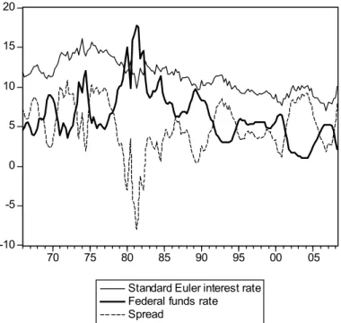
Figure 1 displays the computed standard Euler interest rate and the federal funds rate, as well as the spread between these two rates, vHxohu>pw = UHxohu
w Upw , in percent. The Euler rate uwHxohu averages at11=4 percent, whereas the federal funds rateupw averages at6=5
percent; thus the average spread is 4.9 percentage points. In ation averages at4=4percentage points over the period considered. The federal funds rate and the Euler rate, which should be identical according to standard macroeconomic models, display no apparent co-movement. The federal funds rate is strongly negatively correlated with the spread, a fact that has recently been pointed out by Atkeson and Kehoe (2009), while using Smets and Wouter’s (2007) model. Thus, the unexplained wedge between the federal funds rate and the Euler rate is substantially related to the federal funds rate.At low frequency, the Euler and federal funds rates are positively correlated, which is mainly due to in ation trends (upward in the
1 1
Quarterly data are from the Federal Reserve Bank of St. Louis FRED database and are released by the Federal Reserve Board, the Bureau of Economic Analysis (U.S. Department of Commerce), the Bureau of Labor Statistics (U.S. Department of Labor), and the Census Bureau (U.S. Department of Commerce).
-10 -5 0 5 10 15 20 70 75 80 85 90 95 00 05 Standard Euler interest rate
Federal funds rate Spread
Figure 1: Euler rateuHxohu and federal funds rate up (in %)
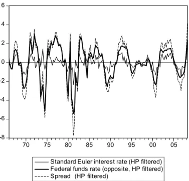
1970s and then downward in the 1980s) that move both rates in the same direction. These trends evidently distort the correlation between the Euler and policy rates in comparison to a theoretical environment with constant steady-state in ation. In order to correct for these in ation trends and to isolate short-run (business cycle) interest rate dynamics from longer term movements, we HP-lter (= 1600) the interest rate series. The correlations between HP-ltered variables will be used to assess theoretical moments of our model, which will be computed for a xed steady-state in ation rate.
Table 1 Empirical correlations for HP-ltered series
Euler rate Debt rate
fruu¡vHxohuw > Upw ¢ 0=98 fruu(vw> Upw ) 0=90 fruu¡UHxohuw > Upw ¢ 0=66 fruu¡Ugw> Upw ¢ 0=57
Figure 2 displays the same variables as in Figure 1 but HP-ltered. The bold line is minus
the detrended federal funds rate. Thus, there is an apparent negative comovement between uctuations of the spread and of the policy rate. Moreover, the Euler and policy rates are also negatively correlated at business cycle frequency. Table 1 presents the correlations for the HP-ltered series, i.e., the (unconditional) correlations between the federal funds rate, the Euler rate, and the spread vHxohu>p (left column). The table further contains correlations
-8 -6 -4 -2 0 2 4 6 70 75 80 85 90 95 00 05 Standard Euler interest rate (HP filtered) Federal funds rate (opposite, HP filtered) Spread (HP filtered)
Figure 2: HP-ltered Euler rateuHxohu and federal funds rates up (in %)
in terms of the closely related debt rate Ugw (and vpw = Ugw Upw ), which corresponds to the Euler rate in our model.12 Three main results should be noted: rst, there is a strong negative correlation (close to minus one) between the spreads and the policy rate. Second, the Euler (debt) rate and the policy rate are negatively correlated as well, though to a smaller extent than the spreads.13 Third, the correlations for the Euler rate and the debt rate are relatively similar.
As emphasized by Atkeson and Kehoe (2009), the apparent mismatch between the Euler and federal funds rates casts severe doubts on the common practice in current macroeconomics to assume that both rates are identical. We will show in the subsequent sections that this behavior of interest rates can be explained by modeling monetary policy in accordance with central bank practice.
1 2Details on this latter rate can be found in the subsequent section and in appendix 8.2. The dierence between the standard Euler equation and the Euler equation in our model is mainly due to a cash-in-advance constraint. Overall, these two rates dier only slightly, except in accelerating in ation (late 1970s) and disin ation (early 1980s) episodes, as well as around 1992 and 2003 with the drops in the policy rate.
1 3
This relates to the results in Canzoneri et al. (2007) for the case ofreal rates. Their correlation between real rates is smaller than the values given in our table 1, and theynd a positive correlation between nominal rates, which is due to the in ation trends, as explained above.
3
The model
In this section we develop a macroeconomic framework where the asset market and open market operations (the money market) are separated. There are four dierent types of agents: households, rms, the central bank and the government. We abstract from nancial intermediation and assume that households directly trade with the central bank in open market operations.
Households can hold short-term government bonds (i.e. T-bills) and non-interest bearing money, and they can borrow and lend among each other using a full set of nominally state contingent claims. Their demand for money is induced by assuming that goods market transactions cannot be conducted by using credit. This is modelled by a cash-in-advance constraint, i.e. by assuming that households have to hold money for goods market purchases. They can get money from the central bank only in exchange for eligible securities in open market operations. To give a preview, nancial markets separation will lead to a spread between the government bond rate and the policy (repo) rate, i.e. a risk premium, whereas the spread between the debt rate and the bond rate, i.e. a liquidity premium, will be due to the special role of government bonds in open market operation.
Throughout the paper, upper case letters denote nominal variables, lower case letters real variables, and variables without an index (lorm) aggregate variables.
3.1
Timing of events
The timing of markets and the specication of open market operations will be important for our results. We will focus on the case where only government bonds are eligible in open market operations. The timing of events in each period is as follows:
A household l enters a period w with nominal assets carried over from the previous periodw1 :
Pl>wK31+El>w31+Gl>w31>
where PK denotes holdings of money, E one-period government bonds, and G one-period state privately issued contingent claims.
1. Aggregate shocks materialize, labor is supplied by households, and goods are produced by rms.
2. Households can then trade money in exchange for eligible assets in open market op-erations. The central bank supplies via outright sales/purchases and via repurchase agreements. The relative price of moneyUpw (for both types of trades) is controlled by the central bank and will be called policy (or repo) rate:
where Ll>w is the amount of money received by household l and El>wf the amount of bonds the central bank gets. We assume that only government bonds are eligible
El>wf El>w31= (3)
When household lleaves the money market, its bond holdings equalEl>w31El>wf . 3. Households enter the (nal) goods market, where money is assumed to be the only
accepted means of payment. Thus goods market expenditures are constrained by money carried over from the previous period plus money acquired from the central bank in current period open market operations:
Swfl>wLl>w+Pl>wK31>
where fl denotes purchases of the nal consumption good and S its price level. When household lleaves the goods market, its money stock equalsLl>w+Pl>wK31Swfl>w. 4. Before households trade in the asset market, current labor income and dividends are
paid back in cash to households. Further, government bonds can be repurchased from the central bank with cash, i.e. household l can repurchase bonds El>wU using money Pl>wU = EUl>w. After repurchase agreements are settled, money and bond holdings of household lequal
f
Pl>w =Ll>w+Pl>wK31+Swzwql>w+Swl>wSwfl>wPl>wU>
e
El>w =El>w31El>wf +El>wU>
where zw denotes the real wage rate,qw working time andSwl>w dividends.
5. Finally, the asset market opens. In the asset market, households receive payos from maturing debt. They can further borrow/lend and trade money and bonds among each other, and they can buy bonds from the government at the price 1@Uw (while the price of money in terms of bonds in the asset market equals Uw). Hence, we can summarize the asset market constraint of household las
(El>w@Uw) +Hw[tw>w+1Gl>w] +Pl>wK Eel>w+Gl>w31+Pfl>w+Sww> (4) where Sww denotes lump-sum government transfers and tw>w+1 is a stochastic discount
factor, which will be dened below. The central bank reinvests its payos from maturing bonds in new bonds and does not change money supply. Since money cannot be issued by the private sector, R fPl>wgl=
R
Pl>wKgl holds.
The total amount of government bonds held by the private sector at the end of the period
R
central bank. In what follows we describe the model in detail.
3.2
Private sector
Households There is a continuum of innitely lived households indexed with l 5 [0>1]. Households have identical asset endowments and identical preferences. Householdlmaximizes the expected sum of a discounted stream of instantaneous utilities x:
H0
"
X
w=0
wx(flw> qlw)> (5)
where H0 is the expectation operator conditional on the time 0 information set, and 5
(0>1) is the subjective discount factor. The instantaneous utility x is assumed to satisfy xw= [(f1l>w31) (1)31]ql>w, where 1and A0.
A household lis initially endowed with money Pl>K31, government bonds El>31, and
pri-vately issued debt Gl>31. As described above, it faces three constraints in each period. In
open market operations, it can acquire additional moneyLl>w up to the amount of government bonds carried over from the previous period Ew31 discounted byUpw . Hence, privately issued debt is not eligible in open market operations, which accords to common practice of central banks (like the BoE or the US-Fed in normal times) to restrict the set of eligible securities mainly to short-term government bonds (see e.g. Meulendyke, 1998). Accordingly, we assume that only government bonds can be used as collateral for money in open market operations, such that household lfaces the following open market constraint
Ll>wEl>w31@Upw = (6) In principle, the central bank can also withdraw money from the private sector (Ll>w ?
0). Here, however, we focus on the empirically relevant case where the central bank cre-ates a “structural deciency” when it supplies money outright (PK),14 by choosing a par-ticular relation between money supplied under repurchase agreements and under outright sales/purchases. This strategy leads to a su!ciently large fraction of money that will be supplied under repurchase agreements to guarantee Ll>w 0 in equilibrium (see below).
Households are further assumed to rely on cash for transactions in the goods market. Given that they can rst trade with the central bank in open market operations, the cash-in-advance constraint diers from Svensson’s (1985) cash-in-advance constraint byLl>w
Swfl>w Ll>w+Pl>wK31= (7)
1 4This strategy has for example been applied by the US-Federal Reserve: "To most eectively in uence the level of reserve balances, the Federal Reserve has created what is called a ’structural deciency’. That is, it has created permanent additions to the supply of reserve balances that are somewhat less than the total need. Then on a seasonal and daily basis, the Desk is in a position to add balances temporarily to get to the desired level." (see "Fedpoint: Open Market Operations", http://www.newyorkfed.org/aboutthefed/fedpoint/fed32.html).
In the asset market, the household receives pay-ofrom maturing assets, can buy bonds from the government, and can trade all assets with other households. It can further borrow and lend using a full set of nominally state contingent claims. Dividing the period wprice of one unit of nominal wealth in a particular state of period w+ 1by the period wprobability of that state gives the stochastic discount factor tw>w+1. The period wprice of a payoGmw in period w+ 1 is then given by Hw[tw>w+1Gmw]. Substituting out the stock of bonds and money held before the asset market opens, Eel>w and Pfl>w, in (4), the asset market constraint of household l reads can be written as
(El>w@Uw) +Hw[tw>w+1Gl>w] +Pl>wK+ (Upw 1)Ll>w (8) El>w31+Gl>w31+Pl>wK31+Swzwql>wSwfl>w+Swl>w+Sww>
where household l0vborrowing is restricted by the following no-Ponzi game condition
lim
v<"Hwtw>w+vGl>w+v 0> (9)
as well as by Pl>wK 0 and El>w 0. The term (Upw 1)Ll>w in (8) measures the costs of money acquired in open market operations: the households receive new cash Ll>w in exchange forUpw Ll>w bonds.
Maximizing the objective (5) subject to the open market constraint (6), the goods market constraint (7), the asset market constraints (8) and (9), for given initial valuesPl>31,El>31,
and Gl>31 leads to the followingrst order conditions for working timeql>w, consumptionfl>w, additional moneyLl>w, as well as holdings of contingent claims, government bonds and money: xl>qw@zw=l>w> (10) xl>fw=l>w+#l>w> (11) Upw ¡l>w+l>w ¢ =l>w+#l>w> (12) w+1 l>w+1 l>w =tw>w+1> (13) Hw £¡ l>w+1+l>w+1 ¢ 3w+11 ¤=l>w@Uw> (14) Hw £¡ l>w+1+#l>w+1 ¢ 3w+11 ¤=l>w> (15) where l>w and #l>w denote the multiplier on the asset and goods market constraint. The conditions (10) and (11) show that l>w A 0 and that a binding goods market constraint (#l>w A 0) distorts the intratemporal consumption-leisure decision in a conventional way, xl>fw+xl>qw@zw = #l>w. Combining (10) and (11) with (15), discloses the standard in ation tax on consumption, which is implied by the cash-in-advance constraint (7):
Throughout, we will repeatedly refer to the rate of return on a nominally risk-free portfolio of claims that deliver one unit of currency in each state. This debt rate Ug
w is given by Ugw = [Hwtw>w+1]31 and thus (see 13)
1@Ugw =Hw[(l>w+1@l>w)@w+1] (17)
The debt rate closely relates to the Euler rate in section 2. It can dier from the standard Euler rate (see 1) solely due to the cash-credit-good friction l>w xl>fw (see 11). To facilitate comparisons, we will report results for both rates, though the Euler rate has no meaningful role in the model.
The open market constraint (6) is associated with the multiplierl>w0, which measures the liquidity value of bonds. When the goods market constraint is binding: #l>w A 0 /
xl>fw+xl>qw@zw A 0 (see 10 and 11), the role of money as a means of payment is positively valued. Likewise, government bonds, as a substitute for money, can also be valued dierently from non-eligible assets; for this, the price of money in terms of bondsUphas to be su!ciently low. Combining (10), (11), and (12), we obtain
l>w = xl>qw zw +xl>fw Up w = (18)
The multiplier on the open market constraint l>w, tends to decline with the policy rate (see 18), since a higher policy rate reduces the amount of money for each unit of bonds supplied to the central bank. The bond pricing equation (14) shows that a rise in this multiplier tends to lower the interest rate on bonds. Hence, a positive liquidity value of bondsl>w A0gives rise to aliquidity premiumbetween the interest rate on bonds and the debt rate,vw=UgwUwA0, as can be seen from (14) and (17), which can be combined to
Ugw Uw = Hw £¡ l>w+1+l>w+1 ¢ @w+1 ¤ Hw[l>w+1@w+1] = (19)
The household’s investment decisions further links the bond rate to the policy rate. It is willing to hold both assets, money and bonds, if the rate of return on bonds compensates for the costs of acquiring new money in the next period. This can be seen by combining (10), (12), (14), and (15) to 1@Uw= Hw £¡ 1@Upw+1¢(xl>fw+1@w+1) ¤ Hw[(xl>fw+1@w+1)] > (20)
implying that the interest rate on bonds equals the expected future policy rate up to rst order. Finally, the transversality conditions for money, bonds, and private debt as well as the following complementary slackness conditions are satised in the household’s optimum
l) 0el>w313w1@Upw ll>w, l>w 0, l>w ¡ el>w313w1@Uwpll>w ¢ = 0, ll) 0ll>w+pKl>w31w31fl>w, #l>w0, #l>w ¡ ll>w+pKl>w313w1fl>w ¢ = 0>
where pKl>w = Pl>wK@Sw, el>w = El>w@Sw, and ll>w = Ll>w@Sw, and (8) and (9) hold with equality. Households are then willing to hold both types of money, i.e. money held under repurchase agreements Pl>wU and under outright sales/purchases Pl>wK. Changes in the composition of money supplied to the private sector might aect the distribution of eligible securities between the private sector and the central bank.
In the following sections, we will particularly be interested in the case where the open market constraint (6) is binding,l>w A0. It should however be noted that this does not imply that scal policy (or total government debt) is decisive for the maximum amount of money supplied. A more elaborate set-up could for example also contain longer term government bonds that are accepted to a smaller extend by the Fed in exchange for money than short-term government bonds (see e.g. Federal Reserve of New York, 2006).15 While we assume, for simplicity, that all one period government bonds are eligible, central banks in practice typically decide on the fraction of eligible securities that they actually accept in open market operations. In fact all main results derived in this paper will not be aected either if we add non-eligible government bonds with longer maturity or if we assume that only a fraction of government bonds are accepted in open market operations.16
Firms To facilitate a reasonable transmission of monetary shocks we allow for imperfectly exible prices. We introduce price stickiness in a simple way following the New Keynesian literature. In particular, we assume that the nal consumption good is an aggregate of dierentiated goods produced by monopolistically competitive rms indexed withm 5[0>1]. The CES aggregator of dierentiated goods is|
31 w = R1 0 | 31
mw gm>with A1, where |w is the number of units of the nal good, |mw the amount produced by rm m, and the constant elasticity of substitution. LetSmw andSwdenote the price of goodmset byrmmand the price index for thenal good. The demand for each dierentiated good is|mw = (Smw@Sw)3|w, with Sw13 =R01Smw13gm. A rm m produces good |m employing the technology:|mw =dwqmw, where 5(0>1),dis a stochastic productivity level satisfying dw=dw3d1exp%d>w,d0, and%d>w is i.i.d. normally distributed with Hw31%d>w = 0 a constant standard deviation vw=ghy=(%d) 0. Hence, labor demand satises
zw=pfmw|mw@qmw> (21)
where pfmw denotes real marginal costs.
We consider a nominal rigidity in form of staggered price setting as in Yun (1995). Each period rms may reset their prices with the probability 1! independently of the time 1 5For example, if we include non-eligible two-period government bonds they would exhibit the period w price 1@Uow = 1@Ugw Hw 1@Ugw+1
, which can be associated with a "term premium" compared to one-period (eligible) government bonds1@Uow$(1@Uw)Hw(1@Uw+1).
1 6In particular, by extending the type of eligible securities or by reducing the fraction of accepted government bonds, the central bank can freely chose its long-run in ation target (see section 3.5 for a discussion).
elapsed since the last price setting. The fraction!5[0>1)ofrms is assumed to adjust their prices with the steady state in ation rate , where w=Sw@Sw31, such that Smw =SK>mw31.
In each period a measure 1 ! of randomly selected rms sets new prices Semw in order to maximize the expected sum of discounted future dividends Swmw = (SmwSwpfw)|mw :
maxSh mwHw P" v=0! vt w>w+v(Semw|mw+vSw+vpfw+v|mw+v), s.t. |mw+v = Semw3Sw+v|w+v. For ! A 0, the rst order condition is given by
e Smw = 1 HwP"v=0!v £ tw>w+v|w+vSw++1vpfw+v ¤ HwP"v=0! v£t w>w+v|w+vSw+v ¤ = (22)
Aggregate output is|w= (SwW@Sw)qw, where(SwW)3=
R1 0 S3 mw gmand thus(SwW)3 =! ¡ SwW31¢3+ (1!)Sew3. Under exible prices!= 0, real marginal costs are given bypfw= %3%1.
3.3
Public sector
The public sector consists of a government and a central bank. The government issues one-period bonds EW, which are held by households and by the central bank. For simplicity, we assume that the supply of government bonds is exogenously determined and is issued at a constant growth rate satisfying
A :EwW =EWw31= (23) It should be noted we do not aim at modelling the evolution of total public debt by (23). Of course, public debt also consists of government bonds with longer maturity that might grow with a rate dierent from , which will not be modelled here to keep the exposition simple. Hence, (23) can be viewed as a supply of a particular asset that the central bank declares eligible rather than a characterization of total public debt. In order to avoid any further eects of scal policy we assume that the government can raise or transfer revenues in a non-distortionary way, Sww. As long as bonds with longer maturities are not eligible (which roughly accords to common central bank practice), we can therefore neglect them without any consequences for the analysis of monetary policy eects.
Accounting for the transfersSwpw from the central bank, the simplied government budget is balanced by
¡
EwW@Uw
¢
+Swpw =EwW31+Sww=
The central bank supplies money in exchange for government bonds in open market operations in form of outright sales/purchases PwK and repurchase agreementsPwU. Before the money market opens, the central bank’s stock of government bonds equals Ewf31 and the stock of outstanding money equals PwK31. It then receives an amount of bonds Ewf in exchange for money Lw, and after repurchase agreements are settled its holdings of bonds reduces by EwU and the amount of outstanding money by PwU =EwU. Before the asset market opens, where
the central bank can invest in government bonds Ewf, it holds an amount of bonds equal to
e
Ef
w =Ewf+Ewf31EwU. Its budget constraint is given by
(Ewf@Uw) +Swpw =Ewf+Efw31EUw +PwKPwK31
¡
LwPwU
¢
=
In accordance with the operational practice of central banks we assume that it rolls over its maturing assets (see e.g. Meulendyke, 1998, ch.7). Thus, we assume that the central bank also enters the asset market at the end of each period, and reinvests in bonds to the amount that equals its current stock of maturing debt Ef
w = Eewf. Further using EUw =PwU andEwf=Upw Lw, the budget constraint can be simplied to(Ewf@Uw)Ewf31=PwKPwK31+
(Upw 1)LwSwpw .
Following common practice (see Meulendyke, 1998), we assume that the central bank transfers interest earnings from asset holdings to the government:
Swpw =Ewf(11@Uw)= (24)
Note that these transfers will not be negative in equilibrium, such that the central bank will never rely on funds from the government.17 Accordingly, its bond holdings will evolve according to EwfEwf31 =Upw Lw ¡ LwPwK+PwK31 ¢ = (25)
Thus the central bank receives more bonds from households, when money supply or the policy rate is high (see 25). The term in brackets on the RHS of (25) accounts for money supplied under repos, which reduces the latter eect.
Regarding the implementation of monetary policy, we assume that the central bank con-ducts monetary policy by using simple instrument rules. The central bank sets the policy rate Upw contingent on its own lags, current in ation, and current real activity, which is measured as in Justiniano and Primiceri (2008). To assess the monetary transmission mechanism, we further consider shocks to the following Taylor-rule-type interest rate reaction function
Upw =¡Upw31¢U(Up)13U(
w@)(13U)((|w@dw)@(|@d))|(13U)exp%U>w= (26) where 0, | 0, U 0 and %U>w is normally i.i.d. with Hw31%U>w = 0and a constant standard deviation vw=ghy=(%U) 0. The long-run policy rate, Up A 1, and the target in ation rate, A , can be chosen by the central bank. Note that the interest rate rule encompasses the case of exogenous interest rate policies, =| = 0, which we found to be consistent with local equilibrium determinacy in cases where the open market constraint (6) 1 7This is dierent in standard models, where central bank transfers seigniorage (dened as the change in the monetary base) to the government in each period. A discussion of government transfers and central bank independence can be found in Sims (2003).
is binding. A short discussion of this property can be found in section 5.1.
In contrast to standard models, where repurchase agreements are not considered, the central bank has an additional role: it can decide on whether money is traded in form of outright sales/purchases or in form of repurchase agreements. For simplicity, we assume that it chooses a constant ratio of money supply under both types of open market operations :
PwU=·PwK> or PU
w =Pw1+ll, where Pw is the total money supply, Pw = PwK+PwU. We assume that
A0to account for the fact that the Trading Desk of the Federal Reserve Bank of New York “structures its outright holdings to maintain a need to routinely add to balances by arranging repurchase agreements” (see Fed New York, 2006). This “structural deciency”, i.e., the choice of an appropriate relation between money supplied under repurchase agreements and under outright sales/purchases, allows the Fed to keep a tight control over the federal funds rate in a exible way.
3.4
Rational expectations equilibrium
In equilibrium, there will be no arbitrage opportunities and markets clear, qw =
R1 0 qmwgm = R1 0 qlwgl and |w = R1 0 |mwgm = R1
0 flwgl = fw. Households will not behave dierently and
aggregate asset holdings satisfy ;w 0 : R01Gl>wgl = 0,
R1 0 P K l>wgl = R1 0 Pfl>wgl = P K w , R1 0 Pl>wUgl = PwU, R1 0 El>wgl = Ew, R1 0 El>wf gl = Ewf> R1 0 Ll>wgl = Lw = PwKPwK31+PwU, and EwW =Ew+Efw.
Since the government bond is the single eligible security, its distribution between the central bank and the private sector will matter. Given that the government issues bonds according to a constant growth rate , household bond holdings change according to Ew Ew31 = (1)EWw31Ewf+Efw31. Further using (25), the evolution of bonds held by households
satises
EwEw31 = (1)EwW31Upw
¡
PwKPwK31+PwU¢+PwU= (27) Thus, private sector holdings of bonds tend to decrease with a higher price of money Up and to increase with . For a given injectionLwhouseholds further loose less bonds when the fraction of money held under repurchase agreements increases.
Throughout, we will focus on the case where the central bank sets its instrument such that the goods market constraint (7) is strictly binding (#w A 0). In the long-run, this is ensured by a su!ciently large in ation target, A (see section 3.5). A rational expectations equilibrium can then be dened as follows:
A rational expectations equilibrium is a set of sequences {fw> qw> |w> zw> pw> ew> eWw> Upw > Ugw> Uw> Sw}"w=0 satisfying the rms’ rst order conditions and the production technology,
goods market constraint Swfw=PwK+PwU, the open market constraint ew31 Upw w pUw +pKw pKw313w1> and ewew313w1 = (1)eWw313w1Upw ¡ pK w pKw313w1 ¢ (Up w 1)pUw, for=eWww@eWw31,
for a monetary policy satisfying (26), given{dw}"w=0 and initial valuesP31 0,E31A0, and
S31 A0.
Note that under a non-binding open market constraint,ew31@wA Uwp
¡
pUw +pKw pKw313w1¢, the evolution of government bonds will neither aect the equilibrium allocation nor the asso-ciated price system. If however the open market constraint is binding,ew31@(Upw w) =pUw + pKw pKw313w1, household bond holdings matter and (27) reduces toEw= (1)EwW31+PwU.
3.5
Steady state
In the following analysis, the two cases of a binding and a non-binding open market constraint (6) will be treated separately, which facilitates analyzing the mechanisms that are responsible for the main results.18 Throughout the analysis, we are particularly interested in the case where the open market constraint is binding. The central bank can conduct monetary policy in a way that ensures the rate of return on government bonds to be lower on average than the rate of return on private debt in equilibrium. This case is consistent with the empirical observation that the policy rate has almost always been below the implied Euler rate (see Figure 1). Households then tend to economize on bond holdings, i.e. they will not hold more government bonds than necessary for their money market trades. If however both returns are identical, households can borrow and invest in government bonds without costs such that the open market constraint will not be binding.19
In order to analyze interest rates and monetary policy for the two regimes in a separate way, we examine steady states with a binding and a non-binding open market constraint. We then assume that monetary policy is conducted in a way that implements one particular steady state and that aggregate shocks are su!ciently small, so that we can analyze the dynamic properties of the economy in the neighborhood of this steady state. A steady state value of an endogenous variable {w will not carry a time index,{.
To examine the two cases, we use (19) which leads to the following steady state condition for the multiplier on the open market constraint 0
@= ³ UgU ´ @U= (28) 1 8
The set of equilibrium conditions for both cases can be found in the appendix 8.2. To simplify the analysis, we disregard the long-run dispersion of prices at in ation rates exceeding one.
1 9
Likewise, if the central bank simply declares both assets as eligible for open market operations, the private sector can freely create any amount of private debt that can be used in exchange for money, such that the private sector never runs out of eligible securities.
Thus a strictly positive spread between the debt rate Ug and the bond rate U implies the multiplier on the open market constraint to be strictly positive A 0. The open market constraint is then binding in the steady state.
Before examining the dierences between both steady states, we look their at common properties. Throughout the paper, we assume that the central bank successfully implements its in ation target in the long-run. The steady state Euler rate is, as usual, determined by (17),Ug=@. Combining (15) and (17) givesUgwHw[l>w+1@w+1] =Hw
£¡ l>w+1+#l>w+1 ¢ @w+1 ¤ , which in steady state demands the multiplier on the cash-in-advance constraint (7) to satisfy
#@=Ug1 (29)
Together withUg=@, condition (29) implies that the cash-in-advance constraint is binding in the steady state, if the in ation target exceeds, A , which will be assumed throughout the analysis. Further using (16), (21), and f= q, shows that steady state consumption is given by f+1@31 = %1 % > (30)
while real balances satisfyp=f> pK+pU=p>andpU=pK. Thus, for axed in ation target A , the steady state valuesUg,f,|=f,q=|1@,p,pk andpU are independent of , i.e. do not depend on the tightness of the money market constraint. Nevertheless, monetary policy is non-neutral in the long-run due to the in ation tax on consumption (see 30) originating in the cash-credit-good distortion induced by the cash-in-advance constraint (7). The following proposition summarizes these properties.
Proposition 1 If the central bank sets the in ation target and the steady state policy rate such that A andUp? @, the goods market constraint and the open market constraint
are binding in the steady state. The equilibrium allocation in the steady state is then identical to the case where the open market constraint is not binding and independent of the policy rate.
The open market constraint only matters for the steady state values for the bond rate Uand for the real value of government bondse.
l=) If the central bank sets the average policy rateUpequal to the debt rateUgin a steady state, Up =@, the interest rate on government bonds U=Up (see 20) also equals Ug. By (28), the multiplier on the open market constraint will then be equal to zero = 0and the steady state is characterized by U= Ug =Up. Since the open market constraint is not binding, there are innitely many values for real bonds consistent with a long-run equilibrium.
ll=) If however the central bank chooses an average policy rate Up that is strictly smaller than Ug, which requires Up ? @, the open market constraint is binding and the
steady state is characterized by U=Up, e
Up =p
K¡1
31¢+pU> (31)
and e= (1)eW31+pU. Combining the latter with (31) andpU=pK, shows that eW will be strictly positive in a non-de ationary steady state. For a realistic in ation target 1, which will be considered throughout the analysis, (23) implies that the in ation target equals the growth rate of short-term government bonds,=. As mentioned before, we do not interpret the equality = (in case ll=) as a restriction for the central bank’s in ation target to depend on public debt: rst,EW just measures the supply of short-term government bonds, while total public debt, of course, also contains long-term bonds that are disregarded in our model for simplicity. And second, the central bank is in principle free to adjust the set of eligible securities, and can thereby chose an in ation target that diers from. If, for example, the central bank chooses a smaller in ation target ?, it can simply accept smaller fractions of government bonds in open market operations. Otherwise, for A, it might also declare other assets (or a fraction of them) as eligible, which grow with a rate that exceeds.20 In any case, the central bank can actually decide on the maximum amount of money that can be traded in open market operations by deciding on the set of eligible securities. Though this is not explicitly modelled in this paper, we can easily account for these arguments by allowing for a richer asset structure, which will nevertheless leave the main results unchanged.
4
Interest rates and spreads
In this section, we examine the relation between the three interest rates, i.e., the policy rate Upw , the bond rateUw, and the debt rateUwg. The bond rate Uw and the policy rateUpw are closely related to each other as can be seen from (20). The spread between these two rates, which can be interpreted as a risk premium, will be examined below. Before, we examine the spread between the debt rate Ugw and the bond rate Uw, which is a liquidity premium. We will show that both the spreadUgwUwand the debt rateUgw itself decrease when the central bank raises the policy rate Up, which is consistent with the empirical evidence provided in section 2.
For the analysis in this section we will use a simplied version of the model, to facilitate the derivation of analytical results. Throughout this section, we assume that production is linear (= 1), the production sector is perfectly competitive ( $ 4), and that prices are
2 0
In light of the decline in the amount of outstanding US-treasury debt, the latter case was in fact viewed as a relevant issue in 2001. See Board of Governors (2001) for a comprehensive discussion on alternative assets that were considered for open market purchases. This issue has regained interest in the currentnancial crises, where the Fed and other central banks relaxed their asset acquisition policy.
perfectly exible (! = 0). We further assume in this section that money is only supplied via repurchase agreements Pw =PwU ($ 4) and that the supply of government bonds is constant (= 1).
4.1
The liquidity premium
Households are willing to hold government bonds even if the bond rate is lower than the debt rate, since bonds exhibit an additional liquidity value (see 19). Due to lower interest earnings, households will economize on bond holdings such that the open market constraint (6) is binding. This property has already been discussed in the previous section, where we have shown that the central bank can implement a long-run equilibrium with a binding money market constraint if the policy rateUpis set at a value lower thanUg=@ (see proposition 1). In the neighborhood of this steady state, the spread between the debt rate and the bonds rate will not be constant over time and will in particular be aected by the monetary policy stance, since the liquidity value of bonds will depend on the money market conditions.
To facilitate an exact analysis of the liquidity premium, we restrict our attention to the case of an exogenous interest rate policy =| = 0. Since the current bond rate is aected by tomorrow’s policy rate rather than today’s policy rate (see 20), we further assume that the policy rate sequence exhibits inertia U A 0.21 A rise in the policy rate Uwp then has two immediate eects. It reduces nominal consumption for a given stock of household bond holdings Ew31 (see 6 and 7). It further leads to lower end-of-period nominal bond holdings
Ew (see 27, which for Pw =PwU and = 1 reduces to Ew = Ew31@Uwp). Thus, both eects tend to reduce in ation. Since the policy rate is raised in an inertial way, in ation is also expected to be lower in the subsequent period, such that households demand a lower debt rate Ugw (see 17).
These results can easily be derived for the simplied version when utility is logarithmic in consumption = 1.22 They are summarized in the following proposition.
Proposition 2 Consider the simplied version, where = 1 and the policy rate satises
=| = 0 and Up ?1@. Then, in the neighborhood of the steady state the debt rate Ugw
and the ratio Ugw@Uw decrease with l=) the current level of the policy rate if U A 0 and ll=)
with the variance of policy rate innovations %U>w. Proof. See appendix 8.3.
The spread UwgUw, i.e., the liquidity premium, originates in the ability of bonds to be convertible into means of payments in open market operations before the goods market opens.
2 1
Under perfectly exible prices both rates,UgandU, will be constant ifU= 0. This will not be the case
for the calibrated version of the model considered in section 5.
2 2As mentioned above, the simplied version is further characterized by= 1,
< ",!= 0,l< ", and
If the costs of exchanging bonds against moneyUwpincreases, the liquidity value of bonds and thus the liquidity premium decline. Similarly, when the variance of the policy rate increases, the liquidity value of bonds becomes more uncertain and the liquidity premium is reduced. Put dierently, when the costs associated with the liquidation of bonds get more risky, the compensating interest rate U increases. This eect resembles the concept of a liquidityrisk
premium (see Acharya and Pedersen, 2005).
According to the standard Fischer (expected in ation) eect, the debt rate Ug falls in response to an increase in the policy rate, since in ation is expected be to lower than average in ation rate in the subsequent period. It should be noted that this in ation response is further responsible for an increase in consumption, since the in ation tax on cash goods is then lowered (see 16). This counterfactual consumption response will disappear when prices are considered to be imperfectly exible (see section 5).
4.2
The risk premium
As discussed in the previous section, the interest rates on bonds and debt only dier when the open market constraint is binding. In contrast, there can be a spread between the policy rate and the bond rate, regardless whether the open market constraint is binding or not. This can be seen from (20), which be rewritten as
1@Uw=Hw ¡ 1@Upw+1¢+fryw £¡ 1@Upw+1¢>(xfw+1@w+1) ¤ Hw[xfw+1@w+1] = (32)
Households are willing to hold both, money and bonds, if the rate of return on bonds compen-sates for the costs of converting bonds into money in next period’s open market operations. Up to rst order, the current bond price 1@Uw, which is determined in the asset market in period w, equals the expected future money-price of bonds in open market operations Hw
¡
1@Up
w+1 ¢
. For the case of a binding open market constraint, the price of a government bond 1@Uw can be shown to be smaller thanHw¡1@Upw+1
¢
. The reason is that the covariance on the RHS of (32) is negative, i.e., the real policy rateUpw+1 is positively related to the mar-ginal utility of consumption divided by the in ation rate, xfw+1@w+1. The spread between
the bond rate and the expected policy rate then tends to be positive and increases with the measure of relative risk aversion. Hence, this spread is a risk premium on the nominal rate of return on bonds compared to the expected policy rate: a risk-averse agent who considers investing in bonds in the asset market will ask for a price 1@Uw that is lower than the ex-pected money-price of bonds in next period’s open market market, if a lower policy rate (and thus a higher pay-ofrom bonds) is expected to be associated with higher consumption and in ation.
To establish this result, we again apply the simplied version of the model (= = 1, ! = 0, $ 4, and $ 4). We now allow for varying degrees of relative risk aversion,
A1, and we focus on white noise technology shocks,d= 0, as the only source of aggregate uncertainty, such that%U>w= 0, while the policy rate will endogenously be adjusted according to A0 and U=| = 0. The following proposition summarizes the main results.
Proposition 3 Consider the simplied version, where A 1 and d = 0, while the policy rate satises A 0, U = | = 0, %U>w = 0 and Up ? 1@. Then, in the neighborhood
of the steady state the current price of government bonds is smaller than the expected future money-price of bonds 1@Uw ? Hw
¡
1@Uwp+1¢. The average bond rate Uw further increases with
the households’ relative risk aversion and with the variance of productivity shocks.
Proof. See appendix 8.4.
The covariance term in (32) is strictly negative under a binding open market constraint, since a higher policy rate tends to reduce current consumption times in ation ew31@Uwp = fww. Then, the bond rate tends to exceed the policy rate and further increases for a given policy rate, if aggregate risk,vw=ghy=(%d), or the degree of relative risk aversion increases. In both cases households are only willing to hold bonds at a higher interest rate U.
5
Numerical analysis
In this section we apply a numerical analysis of a calibrated model. Werst describe how we calibrate the model, then we re-examine the behavior of interest rates, andnally we explain the transmission of monetary policy shocks.
5.1
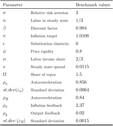
Parameter values
To allow for responses of consumption and in ation that are more realistic than before, we consider imperfectly exible prices, ! A 0. For most of the model’s parameter we apply standard values for quarterly data (see table A1 in appendix 8.5). In particular, we set the inverse of the elasticity of intertemporal substitution, the labor income share, the fraction of non-optimally price adjusting rms !, and the elasticity of substitutionequal to = 2, = 2@3, ! = 0=8, and = 6, while is adjusted to get a steady state value of working time equal to q = 1@3. The parameters for the stochastic productivity process are taken from Schmitt-Grohe and Uribe (2007) and are given by d= 0=856and vw=ghy=(hd) = 0=0064. The policy rate is set according to an inertial Taylor rule (see 26), where we used parameter values estimated by Justiniano and Primiceri (2008) for 1984—2004: U = 0=84, = 2=37, | = 0=02, and vw=ghy=(hU) = 0=0015.
Throughout the analysis, we restrict our attention to locally determined equilibria. When the open market constraint is not binding, our model reduces to an almost standard New Keynesian model and local equilibrium determinacy requires interest rate policy to satisfy the Taylor-principle (like the inertial Taylor-rule). If however the open market constraint is binding, we nd that local equilibrium determinacy applies regardless whether interest rate
policy satises the Taylor principle or is exogenous. We will then also apply an exogenous policy (>| = 0 and U = 0=84) to isolate eects of exogenous interest rate changes from eects due to endogenous interest rate adjustments. The reason why local equilibrium de-terminacy does not rely on an active policy in this case, is that a bounded supply of eligible securities (23) serves as a nominal anchor similar to the stock of money under a money growth policy.23
To match the average interest rate presented in section 2, we apply a target quarterly policy rate equal toUp= 1=0651@4= 1=0159, a (quarterly) debt rate equal toUg= 1=1141@4 = 1=0274, leading to a spread v= 0=0115, and a in ation rate equal to = 1=0441@4 = 1=0108.
The steady state values for Ug and are linked by the Euler equation, which in the steady state readsUg=31(1+f), wherefis the steady state consumption growth rate. While real consumption growth rate fis strictly positive in the data, it is neglected in the model, for simplicity. We therefore set the discount factorequal to = 0=984, which is smaller than values usually applied in the business cycle literature, to compensate for a positive steady state consumption growth rate (see also King et al., 2002). It turns out that the choice of does not signicantly aect the quantitative results. Finally, we chose 1=5 for the policy parameter to match the observed ratio between total reserves and reserves supplied under repurchase agreements. This ratio was almost constant in the 2000s before the crisis24.
5.2
Interest rate behavior
In this section we again take a look at the interest rates, which have already been analyzed qualitatively in section 4. Here, we relate the results of the simulated model to the analytical results presented in proposition 2 and 3 and to the empirical evidence presented in section 2. To account for the eects of second moments on asset prices, we apply a second order approximation at the deterministic steady state (see Schmitt-Grohé and Uribe, 2004).25
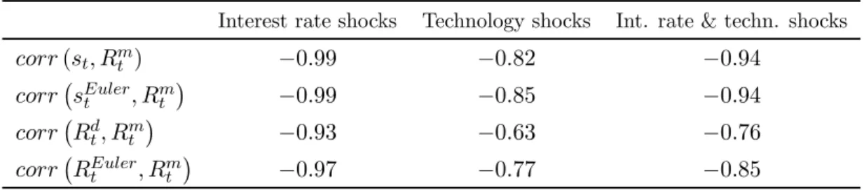
The main properties of the debt rate and the liquidity premium are summarized in propo-sition 2. Consistent with the empirical evidence provided in section 2, it implies that both are negatively correlated with the policy rate. To prove this claim we neglected technology shocks. Here, we examine the magnitude of the correlations for the calibrated model, where technology shocks are also considered. Table 2 presents the correlation between the debt rate and the policy rate as well as the correlations between the spread H0vw=H0
¡
Ugw Uw
¢
and the policy rate. It further contains the corresponding values for the Euler rateUHxohuw and the 2 3This property of our model is in fact closely related to the determinacy property of the cash-in-advance model with sticky prices derived in Adao et al. (2003), who examine the case where both, the nominal interest rate and the supply of money are controlled by the central bank at the same time. A local determinacy analysis for our model is available upon request from the authors.
2 4See Federal Reserve Bank of New York, Domestic Open Market Operations, various issues, and FRED database.
spread H0vHxohuw = H0 ¡
UHxohuw Uw
¢
, where UHxohu is the rate implied by a standard Euler equation, Hw[xf>w+1@(xf>ww+1)] = 1@UHxohuw ; the latter has no meaningful role in our model and is only computed to facilitate comparisons.26
The correlations are highly negative when only interest rate shocks are considered (second column), while they are less pronounced when only technology shocks are considered (third column). When we consider both types of shocks, the correlations take intermediate values (see last column). Overall, the correlations between the spreads and the policy rate are larger in absolute terms than the correlations between the debt rate (or Euler rate) and the policy rate. In sum, the correlations presented in table 2 come close to the empirical correlations presented in table 1 in section 2.
Table 2 Unconditional correlations of HP-ltered series (= 1600)
Interest rate shocks Technology shocks Int. rate & techn. shocks
fruu(vw> Uwp) 0=99 0=82 0=94
fruu¡vHxohuw > Upw ¢ 0=99 0=85 0=94
fruu¡Ugw> Uwp¢ 0=93 0=63 0=76
fruu¡UHxohuw > Upw ¢ 0=97 0=77 0=85
With the parameter values discussed above, the liquidity premium vw (measured in term of the debt rate) exhibits a mean value equal to 490 basis points in terms of annualized rates. In accordance with the second claim in proposition 2 it declines with the variance of policy rate innovations%U>w. Increasing the standard deviation of policy rate innovationsvw=ghy(hU)from
0=0015 to 0=003 and to 0=006 indeed reduces the mean spread from 490 to 489 and to 487, respectively. This eect is more pronounced (488 and 483) when the policy rate is assumed to follow an exogenous process.
As summarized in proposition 3, the risk premium, i.e. the spread between the bond rate and the policy rate, has been shown to increase with the standard deviation of the productivity shock vw=ghy=(%d) and the relative risk aversion . These eects are also found in the calibrated version, while the size of the risk premium is extremely small (0=064 basis points for the benchmark parametrization and 0=095 basis points for = 5). We expect that this spread can be increased if other sources of risk, e.g. shocks related to nancial intermediation (see Christiano et al., 2007), are also considered in the model, which is beyond the scope of this paper.
2 6
Here we followed the exposition in proposition 1 and computed spreads for the bond rate. Corresponding spreads for the policy rate are almost identical.
5.3
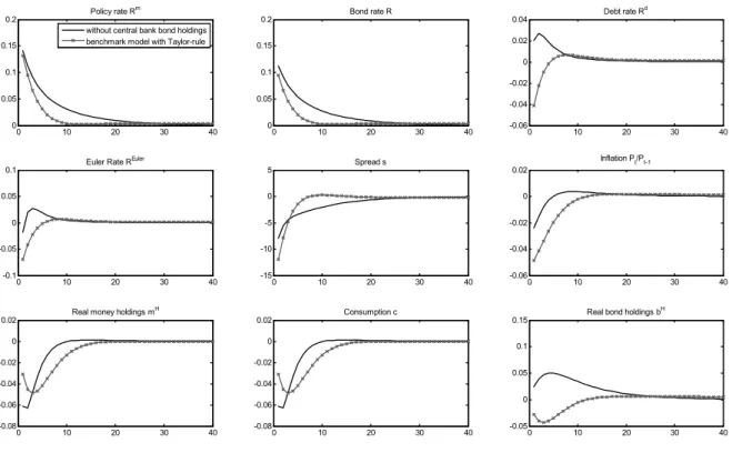
Monetary transmission
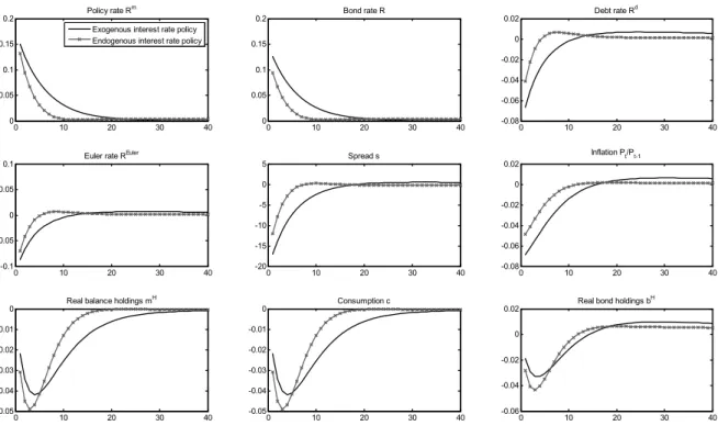
In this section we analyze the monetary transmission mechanism. Consider a positive inno-vation to the policy rate satisfying (26). Figure 3 presents the impulse responses of interest rates and macroeconomic aggregates for the case where the policy rate is set exogenously ( =| = 0and U= 0, black solid line) and for the case where it follows the Taylor type feedback rule (U= 0=84, = 2=37, | = 0=02, red marked line). An increase of the policy rate by 15 basis points (or 60 basis points in terms of annualized rates) from its steady state value leads to a rise in the bond rate on impact by less than 15 basis points, since the current bond rate tends to increase with the future expected policy rate (see 32). In contrast, the debt rate Ugw falls on impact and is closely followed by the Euler rate UHxohu. The spread between the debt rate and the bond rate decreases. Both responses are consistent with the claims made in proposition 1. On impact the spread falls by up to 17% of its steady state value.
Regarding the consumption response, gure 3 further shows that consumption (which equals output,|w=fw) declines in a hump-shaped way, which is qualitatively consistent with VAR evidence (see Christiano et al., 1999). The hump-shaped decline of consumption implies a fall in its growth rate. This pattern, together with the decline in in ation, is consistent with a fall in the Euler rate and the debt rate. Notably, hump-shaped impulse responses can usually not be observed in response to policy rate shocks in simple sticky price models. In these models consumption typically falls on impact and returns monotonically to its steady state value, which is consistent with an increase in the consumption growth rate (see also
gure 5 below).
Hump-shaped responses can of course also be generated by sticky price models that con-tain further features like habits or additional frictions (see Bernanke et al., 1999 or Christiano et al., 2005). Here, the shape of the consumption response is mainly driven by households’ holdings of eligible securities. To get an intuition for this, consider an inertial rise in the policy rate. Due to the higher relative price of money, households can get less cash in the same period such that consumption and in ation fall on impact. While the fall in in ation t