Novel Approach for Neighbourhood-based Collaborative Filtering

(1)

A Novel Approach for

Neighbourhood-based Collaborative

Filtering

Thesis submitted in partial fulfilment of the requirements for the degree of

Bachelor of Technology

in

Computer Science and Engineering

by

Nitesh Agrawal

(Roll: 111CS0117)

under the supervision of

Dr. Korra Sathya Babu

and

Dr. Bidyut Kumar Patra

NIT Rourkela

Department of Computer Science and Engineering National Institute of Technology Rourkela

Rourkela-769 008, Orissa, India

(2)

Declaration

This thesis is a presentation of my original research work. Wherever contribu-tions of others are involved, every effort is made to indicate this clearly, with due reference to the literature, and acknowledgement of collaborative research and discussions. I hereby declare that this thesis is my own work and effort and that it has not been submitted anywhere for any award. The interpretations put forth are based on my reading and understanding of the original texts and they are not published anywhere in the form of books, monographs or articles. The other books, articles and websites, which I have made use of are acknowledged at the respective place in the text. For the present thesis, which I am submit-ting to NIT Rourkela, no degree or diploma or distinction has been conferred on me before, either in this or in any other University. I bear all responsibility and prosecution for any of the unfair means adopted by me in submitting this thesis.

Nitesh Agrawal (111CS0177) NIT, Rourkela.

(3)

Acknowledgement

I take this opportunity to express my gratitude to my guide Dr. Korra Sathya Babu for his guidance and motivation throughout the course of this project. I convey my regards to Dr. Bidyut Kumar Patra without whose technical guid-ance this project would have been a distant aim. I would like to thank my parents for supporting me and showing confidence in me whenever I lost hope. I express my profound gratitude to Almighty and my sisters for their support without which this task could have never been accomplished.

(4)

List of Figures

4.1 Mean asboulte error vs number of neighbours for 100K data set. 16

4.2 Mean asboulte error vs number of neighbours for 1M data set. . 16

4.3 MAE for good items vs number of nieghbours for 100K dataset . 17 4.4 MAE for good items vs number of nieghbours for 1M dataset . . 17

4.5 RMSE vs number of nieghbours for 100K dataset . . . 18

4.6 RMSE vs number of nieghbours for 1M dataset . . . 18

4.7 Precision vs number of nieghbours for 100K dataset . . . 19

4.8 Precision vs number of nieghbours for 1M dataset . . . 19

4.9 RECALL vs number of nieghbours for 100K dataset . . . 20

4.10 RECALL vs number of nieghbours for 1M dataset . . . 20

4.11 F1-score vs number of nieghbours for 100K dataset . . . 21

4.12 F1-score vs number of nieghbours for 1M dataset . . . 21

4.13 Mean asboulte error vs number of neighbours for 100K data set. 22 4.14 Mean asboulte error vs number of neighbours for 1M data set. . 23

4.15 MAE for good items vs number of nieghbours for 100K dataset . 24 4.16 MAE for good items vs number of nieghbours for 1M dataset . . 24

4.17 RMSE vs number of nieghbours for 100K dataset . . . 25

4.18 RMSE vs number of nieghbours for 1M dataset . . . 25

4.19 Precision vs number of nieghbours for 100K dataset . . . 26

4.20 Precision vs number of nieghbours for 1M dataset . . . 26

4.21 RECALL vs number of nieghbours for 100K dataset . . . 27

4.22 RECALL vs number of nieghbours for 1M dataset . . . 27

4.23 F1-score vs number of nieghbours for 100K dataset . . . 28

(6)

Abstract

Recommender systems hold an integral part in online marketing. It plays an important role for the websites that provide the users an environment to rate and review the products. Several methods can be used to make recommender systems, like content-based fil-tering, collaborative filtering [1], hybrid approach, which combines content-based as well as collaborative filtering. Collaborative filter-ing is the most widely used technique to deal with recommender systems. Matrix factorization and neighbourhood approach are the techniques that can be used while dealing with collaborative filter-ing. Both the methods depends on the ratings that the user has provided in the past. Here we concentrate on neighbourhood ap-proach.

Neighbourhood approach depends on the similarity between items [4] or similarity between users [5], depending on which prediction for an unrated item can be made. The similarity between users or simi-larity between items can be computed to provide recommendations. Some of the widely used techniques are the Pearson correlation, cosine-based similarity, adjusted cosine, etc. In this thesis a new approach to find similarity between items is used, here the similar-ity between items is calculated using a modified singularsimilar-ity measure. In this approach, the singularity of ratings provided by each user is taken into consideration [2]. By, using this method recommendation can be found with greater efficiency compared to other existing al-gorithms as this technique uses the contextual information present in the data.

Keywords:Collaborative filtering; similarity; singularity; pre-diction .

(7)

Notations

Ru,i = rating provided by user u to itemi. ¯

Ru = Average of the ratings provided by useru. ¯

Ri = Average of the ratings provided to item i.

I = Column vector of ratings of item i.

similarity(i, j) = similarity between items i and j.

similarity(u1, u2) = similarity between users u1 and u2.

Pu,i = predicted rating for user u on item i.

S_px = singulairty of positive ratings provided by user x.

(8)

Chapter 1

Introduction

Recommendation systems changed the way in which websites inter-act with users. Rather than having a static experience, in which user searches for a product manually and then buy it, recommender system automates the process. Recommender system automatically provides the user options to buy products, based on their past choice. As the number of users and items are increasing exponentially, an appropriate algorithm is required which could provide recommenda-tions with greater accuracy.

s Collaborative filtering is one among the techniques that are used for this purpose. It can be done using matrix factorization or us-ing neighbourhood approach. Each of these processes requires past ratings provided by the users.

1.1 Types of Collaborative Filtering

There are generally two types of methods that are used for collabo-rative filtering i.e matrix factorization and neighbourhood approach.

1.1.1 Matrix Factorization

It is a method based on the principle of extraction of latent features underlying the interaction of user and items [11]. For example, two users give high rating to a particular book if the book is a fiction novel, or they like the writer of the book. Hence, if these latent fea-tures are discovered, predicting rating for the user for any particular item can be easily carried out, because the features associated with the users must match with the features associated with the item. While discovering different features, it is assumed that number of

(9)

features are less than the number of users and number of items. It might suffer from the cold start problem, if the user-item rating matrix is sparse then discovering the features might be difficult.

1.1.2 Neighbourhood approach

This approach is based on finding the neighbours of an item (item-based), or a user (user-based) to get the prediction for an unrated items. To find the neighbours, similarity between items, or users needs to be calculated. It is based on the principle that similar users rate the items similarly, or similar items are rated similarly.

User Based Collaborative Filtering

It is based on the concept of like-minded users [3, 5]. In this ap-proach, ratings provided by users are studied and the pattern is then compared to find similarity between them. It is assumed that like-minded users would rate the item similarly. Therefore, find-ing the neighbours of each user is the aim of this approach. After the neighbours have been found out, their similarity is used in pre-diction of the unrated items for the particular user. This method suffers from drawback as, number of users increases exponentially therefore identifying neighbours for each user might require a great deal of computation, which would make the process of similarity calculation too slow and even less efficient.

Item Based Collaborative Filtering

It is based on considering the similarity between items [1, 4]. Items are said to be similar is they have been voted similarly by the dif-ferent set of users. It looks for the collection of items that the user might have rated in the past, and then the comparison is made to find out how the unrated items are similar to these rated items us-ing various similarity measures. After the similarity between items has been found out, the prediction is made. An advantage of this approach is number of growing users will not affect the efficiency of this approach to a greater extent, and even then less computation will need as compared to user-based approach.

(10)

1.1.3 Challenges in collaborative filtering

• Collaborative filtering algorithms works using the past ratings provided by the users, but the user-item matrix provided is large and is sparse one. The sparsity of the matrix may lead to the cold start problem, where the sufficient amount of past rating by the user is unavailable to predict the rating for any other items, thereby leading to irrelevant predictions [1].

• As the number of users and items increases, the collaborative filtering algorithms suffer from scalability issues.The complex-ity of algorithms is high, and it becomes difficult to handle the huge set of data, thereby increasing the demand for clus-ter computing. Separate mapper and reducer programs can be made to scale the algorithm, maintaining its efficiency.

• There is a tendency among people to give high rating to their own items and provide low rating to others; it causes a major blunder in recommender systems that use collaborative filter-ing.

1.1.4 Problem Statement

The goal is to predict the ratings for the items that user has not rated and to achieve this goal, similarity between items are calculated and prediction is done, so that the recommendation can be provided with greater efficiency as compared to traditional methods like, Pearson correlation, cosine-based and, adjusted cosine.

1.1.5 Contribution

This thesis focuses on neighbourhood approach of collaborative fil-tering algorithms. Here, an improvement of traditional methods is suggested which gives the better quality of recommendations.In the proposed method, the similarity between items is taken into consid-eration along with the contextual information that are derived using singularity of the ratings provided by each user. Later, comparison of the proposed algorithm is carried out with traditional algorithms, proving its efficiency.

(11)

1.1.6 Organization of Thesis

• Chapter 2, gives the literature survey that includes the review of works of existing algorithms to find similarity.

• Chapter 3, deals with the description of proposed algorithm.

• In chapter 4,results of various implemented algorithms and pro-posed algorithms are discussed.

• Chapter 5,presents the conclusion drawn from the results as well as the scope for future work is discussed.

(12)

Chapter 2

Literature Survey

An extensive research is been done in the field of recommender sys-tems and number of methods have come up, each having its advan-tages and disadvanadvan-tages.

Sarwaret al. [1] proved that the item-item scheme provides bet-ter quality of predictions than user-user scheme. The improvement in quality is consistent over different neighbourhood size. Another observation is that the item neighbourhood is fairly static, which can be potentially pre-computed, which results in very high online performance.

Bobadillaet al. [2] proposed that recommender systems contains information that are not used by traditional metrics, but singularity based approach provides a method to use those information thereby increasing the accuracy of similarity measurement techniques The similarities are computed providing a weight to each rating, i.e., sin-gularity. More singular items should have high value in similarity computation as compared to items that are less singular.

Choi et al. [3] described that traditional systems use only simi-larity between users, irrespective of simisimi-larity between items. But, if the similarity between users for a target item is calculated, tak-ing into consideration the similarity of the target item with other items, then the accuracy of the recommender system was seen to be improved.

(13)

2.1 Methods of Similarity calculation

Number of methods are available for similarity computation. Some of them are:

2.1.1 Pearson Correlation

In this similarity measure, similarity is found between any two items

i andj keeping in mind that a particular user has rated both of these items. Advantage of this approach is that calculation in not done for all the users, conditions where customers have rated both the items i and j are only evaluated[1].

similarity(i, j) = P u∈U(Ru,i−R¯i)(Ru,j−R¯j) ( q P u∈U(Ru,i−R¯i)2 q P u∈U(Ru,j−R¯i)2) (2.1)

Here, Ru,i is rating provided by user u to item i. ¯Ri is Average of the ratings provided to item i.

2.1.2 Cosine-based Similarity

The concept of angle is used here to calculate the similarity among the different items [1]. The similarity between the two items is calcu-lated by finding out the cosine of the angle between them. Formally, in the n x m rating matrix (that is user-item matrix), similarity be-tween any pair of items is, denoted by

similarity(i, j) = cos(θ) = I·J

kIk2_k_I_k2 (2.2)

I and J are the column vectors of ratings of item i and item j

respectively.

Its is simple to evaluate. It gives the value in between [0,1]. The variation in the ratings given to the items between the different users is not taken for the computation.

(14)

2.1.3 Adjusted Cosine

In this similarity measure, the difference in the rating scale between different users is taken into account by subtracting the average rat-ing of user form each co-rated pair [1].

similarity(i, j) = P u∈U(Ru,i−R¯u)(Ru,j−R¯u) ( q P u∈U(Ru,i−R¯u)2 q P u∈U(Ru,j−R¯u)2) (2.3)

2.1.4 Similarity based on singularities

Here, similarity between users u1 and u2 is calculated taking into considertaion the singularity of items [2]. This technique, provides the benefit that could lower the weightage of item that has generally been rated high or low.

similarity(u1, u2) = k1 +k2 +k3

3 (2.4)

where,

k1, k2, k3 are defined as,

k1 = P i∈A(1−(Ru1,i−Ru2,i)2)(sip)2 |A| k2 = P i∈B(1−(Ru1,i−Ru2,i)2)(sip)(sin) |B| k3 = P i∈C(1−(Ru1,i−Ru2,i)2)(sin)2 |C|

2.1.5 Similarity between users taking item based similar-ity as weight

Here, similarity between users u1 and u2 is calculated,but using the similarity between the items as a weight to it [3]. This approach

(15)

gives better results, as the similarity betwen users is calculated keep-ing in mind the similarity between items as well.

similarity(u1, u2) = Pm j=1t12∗t2∗t3 q Pm j=1(t1∗t2)2 q Pm j=1(t1∗t3)2 (2.5) where,

t1, t2, t3 are defined as,

t1 =Isim(i, j)

t2 = (Ru1,j−R¯u1)

t3 = (Ru2,j−R¯u2)

Here, Isim(i, j) is the similarity between itemsi and j.

2.2 Methods of prediction calculation

After calculating similarity between items, the prediction can be calculated using following methods [1, 2].

Pu,i = Pk j=1similarity(i, j)∗Ru,j |Pk j=1similarity(i, j)| (2.6)

Here prediction of item i for any user u is calculated by taking into consideration other items that the particular user has rated, and how similar are those items to the item for which prediction is to be done. Pu,i = ¯Ru+ Pk j=1similarity(i, j)∗(Ru,j−R¯j) |Pk j=1similarity(i, j)| (2.7)

Here, prediction of item i for any user u is calculated by taking into consideration the other items, that the particular user has rated,

(16)

and how similar are those items to the item for which prediction is to be done.Also, this method considers the average rating that the item has got by all the users, and on an average what is the rating that the user under consideration gives to the items.

(17)

Chapter 3

Proposed Work

Singularity-based approach uses the contextual information present, which other collaborative filtering algorithms ignore. In this ap-proach singularity of the ratings given by each user is calculated. If a user gives high rating to all the items or low ratings to all the items (i.e., same rating to all the items) then considering that user for calculation of similarity between items will not be beneficial; whereas, if a user has rated only two items differently to the rest of items, then similarity between those two items can be calculated easily. The singularity information obtained can be combined as a weight while calculating the similarity between items, thereby less-ening the worth of user who rates almost all items similarly. This method is based on the hypothesis that value of similarity must be modulated by the value of singularity, in such a way that very sin-gular similarity should be given a higher value.

The ratings provided by users are categorised into relevant rating i.e., rating >= 4 and non-relevant rating i.e., rating < 4. Now, in calculation of similarity between two items a user can rate both the item as relevant (case A), one item as relevant and other as non-relevant (case B), both items as non-non-relevant (case C). Taking all the 3 cases into consideration we have to calculate the similarity between items, and accordingly apply the value of singularity to it. Here, U is set of all the users and N is set of all the items. T is the total number of items rated by a particular user. Px and Nx are the number of positive and negative ratings provided by the user x.

(18)

Algorithm 1Modified Singularity-based Collaborative Filtering

Input : Rating matrix

Output : Prediction matrix

1: procedure_{Modified Sigularity}

2: forall usersx∈U do

3: S_px←1−Px T (3.1) S_nx←1−Nx T (3.2) 4: end for

5: forall itemsi∈N do

6: forall itemsj ∈N do

7: d1← P x∈A(1−(Rx,i−Rx,j)2)(sxp) 2 |A| 8: d2← P x∈B(1−(Rx,i−Rx,j)2)(sxp)(sxn) |B| 9: d3← P x∈C(1−(Rx,i−Rx,j)2)(sxn) 2 |C| 10: similarity(i, j)← d1 +d2 +d3 3 (3.3) 11: end for 12: end for

13: forall usersu∈U do

14: forall itemsi∈N do

15: if Ru,i= 0then

Pu,i← Pk

j=1similarity(i,j)∗Ru,j

|Pk

j=1similarity(i,j)| 16: or

Pu,i←R¯u+ Pk

j=1similarity(i,j)∗(Ru,j−R¯j)

|Pk

j=1similarity(i,j)| 17: end if

(19)

Chapter 4

Results and Analysis

4.1 Evaluation Metrics

• Mean Absoulte Error:MAE is a measure of deviation of rec-ommendations from their true user-specific value. For each rating-prediction pair < Pi, Qi > this metric treats the abso-lute error between them , i.e, |Pi −Qi| equally. The MAE is computed by first summing these absolute errors of the N corresponding ratings-prediction pairs and then computing the average [1, 2, 3, 7]. Formally,

MAE =

PN

i=1|Pi−Qi|

N (4.1)

The lower the MAE,the more accurately the recommendation engine predicts user ratings.

• Mean Absoulte Error for good items:Mean absolute error is calculated only for those items which have positive ratings in the test set.

• Root Mean Square Error:It is a metric represented by the square root of the average of the squares of the differences be-tween actual and estimated preference values. [7]

RMSE =

s PN

i=1(Pi−Qi)2

(20)

• Precision and recall:The precision is the proportion of rec-ommendations that are good recrec-ommendations, and recall is the proportion of good recommendations that appear in top recommendations [2, 3, 7].

• F1-score:The F-Score or F-measure is a measure of a statistic test’s accuracy. It considers both precision and recall measures of the test to compute the score. We could interpret it as a weighted average of the precision and recall, where the best F1 score has its value at 1 and worst score at the value 0 [2, 3, 7].

F1 = 2∗precision∗recall

precision+recall (4.3)

4.2 Data-sets Used

Movie lens datasets are used. It contains ratings in the scale of 1-5.

• 100K data : The full data set consists of 100000 ratings by 943 users on 1682 items. Each user has rated at least 20 movies. Users and Items are numbered consecutively from 1. 80% of the ratings are used as the training set and rest 20% as the test set.

• 1M data: The full dataset contains 1,000,209 anonymous rat-ings of 3,952 movies made by 6,040 Movie Lens users who joined Movie Lens in 2000. 80% of the ratings are used as the training set and rest 20% as the test set.

4.3 Observations

4.3.1 Method 1 (without averaging)

Prediction calculation is done using:

Pu,i = Pk

j=1similarity(i,j)∗Ru,j

|Pk

(21)

Mean Absolute Error

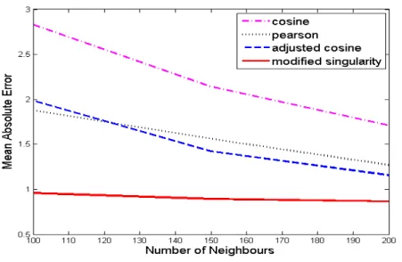
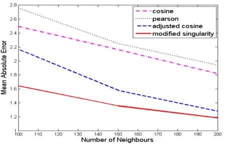
Figure 4.1: Mean asboulte error vs number of neighbours for 100K data set.

Mean Absolute Error

Figure 4.2: Mean asboulte error vs number of neighbours for 1M data set.

• Mean absolute error was found to reduce as the number of neighbour increases. Among all the methods, modified sin-gularity approach was found to have least MAE value with adjusted cosine, Pearson correlation and cosine approaches

(22)

fol-lowing it.

MAE For Good Items

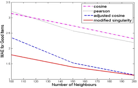
Figure 4.3: MAE for good items vs number of nieghbours for 100K dataset

MAE For Good Items

Figure 4.4: MAE for good items vs number of nieghbours for 1M dataset

• Here, only good items are considered to calculate the MAE values. The resulting graph shows less MAE for modified

(23)

sin-Singularity method works well in the prediction for good items as well.

ROOT MEAN SQAURE ERROR

Figure 4.5: RMSE vs number of nieghbours for 100K dataset

Figure 4.6: RMSE vs number of nieghbours for 1M dataset

• The root mean square value of singularity based approach was observed to be less than other methods , thereby proving the

(24)

efficiency of the process.

• Precision,recall and F1 score were computed and the observa-tions are as follows:

PRECISION

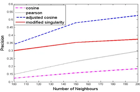
Figure 4.7: Precision vs number of nieghbours for 100K dataset

PRECISION

(25)

The precision of the adjusted cosine method was found to be better followed by modified singularity, Pearson and cosine ap-proaches.

RECALL

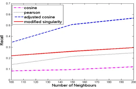
Figure 4.9: RECALL vs number of nieghbours for 100K dataset

RECALL

Figure 4.10: RECALL vs number of nieghbours for 1M dataset

(26)

pro-portion of good recommendations appear in top recommenda-tions using this method followed by modified singularity, Pear-son and cosine approaches.

F1-SCORE

Figure 4.11: F1-score vs number of nieghbours for 100K dataset

F1-SCORE

(27)

ter than the modified singularity method and Pearson and cosine following it.

4.3.2 Method 2 (with averaging)

We calculate prediction by:

Pu,i = ¯Ru+ Pk

j=1similarity(i,j)∗(Ru,j−Rj¯)

|Pk

j=1similarity(i,j)| Mean Absolute Error

(28)

Mean Absolute Error

Figure 4.14: Mean asboulte error vs number of neighbours for 1M data set.

• Mean absolute error was found to reduce as the number of neighbour increases. Among all the methods, modified sin-gularity approach was found to have least MAE value with adjusted cosine, Pearson correlation and cosine approaches fol-lowing it.

• For good items singularity based approach gave better results as compared to other approaches.

(29)

MAE For Good Items

Figure 4.15: MAE for good items vs number of nieghbours for 100K dataset

MAE For Good Items

Figure 4.16: MAE for good items vs number of nieghbours for 1M dataset

Here, only good items are considered to calculate the MAE values. The resulting graph shows less MAE for modified sin-gularity method as compared to other three methods.Modified Singularity method works well in the prediction for good items

(30)

as well.

Figure 4.17: RMSE vs number of nieghbours for 100K dataset

Figure 4.18: RMSE vs number of nieghbours for 1M dataset

• The root mean square value of singularity based approach was observed to be less than other methods , thereby proving the

(31)

• Precision,recall and F1 score were computed and the observa-tions are as follows:

PRECISION

Figure 4.19: Precision vs number of nieghbours for 100K dataset

PRECISION

Figure 4.20: Precision vs number of nieghbours for 1M dataset

Modified singularity method showed the higher value of preci-sion when 1M dataset is used thereby proving that more

(32)

pro-portion good of recommendations appear in top recommenda-tions.Other three methods showed recall lower than the pro-posed method.

RECALL

Figure 4.21: RECALL vs number of nieghbours for 100K dataset

RECALL

(33)

thereby proving that more proportion of recommendations is good recommendations.Other three methods showed precision lower than the proposed method.

F1-SCORE

Figure 4.23: F1-score vs number of nieghbours for 100K dataset

F1-SCORE

Figure 4.24: F1-score vs number of nieghbours for 1M dataset

(34)

dataset was used, thereby proving the efficiency of the method as compared to other three methods that showed lesser F1-score as compared to it.

4.4 Discussion

The results obtained from the proposed similarity measure (singularity-based) are improved vastly as compared to tradition similarity al-gorithms, i.e., Pearson correlation, cosine-based, adjusted cosine. Improvements are especially noticeable in the mean absolute error, root mean square error, MAE for good items. In both the methods of prediction calculation used, with both the datasets, these param-eters were far better as compared to traditional similarity metrics. F1-score of the proposed algorithm was observed to be similar to the adjusted cosine or even worse in certain cases, adding a drawback to the proposed similarity calculation technique. An improvement in F1-score was observed when 1M data set was used and prediction calculation with averaging was done. Precision for the proposed technique was found to be better as compared to other techniques when prediction calculation with averaging was used , but using prediction calculation without averaging precision of adjusted co-sine was observed to be better. Recall of the adjusted coco-sine based approach was found to be better in almost all the cases.

(35)

Chapter 5

Conclusion and Future

Scope

From the above observations, it can be concluded that, MAE, MAE for good items and RMSE for singularity based approach was found to be better than other approaches in all the cases. F1-score for sin-gularity based approach was found comparative to or in some cases poor than adjusted cosine based similarity measure, except when using prediction calculation with averaging, where it was observed to perform better. As a future work, one can try to improve the F1-score, and also this algorithm can be implemented using Hadoop cluster (using map-reduce programming) as it requires high compu-tation to be done. Also, appropriate division of ratings into positive and negative set can be studied to get better results.

(36)

Bibliography

[1] Badrul Sarwar, George Karypis, Joseph Konstan, and John Riedl.“ ItemBased Collaborative Filtering Recommendation Al-gorithms”. Proceedings of the 10th international conference on World Wide Web. Pages 285-295, 2001.

[2] Jesus Bobadilla, Fernando Ortega, Antonio Hernando.“A collab-orative filtering similarity measure based on singularities”. Infor-mation Processing and Management,Volume 48, Issue 2. Pages 204-217, 2012.

[3] Keunho Choi, Yongmoo Suh.“A new similarity function for selecting neighbors for each target item in collaborative filter-ing”.Knowledge-Based Systems.Pages 146-153, 2013.

[4] M. Deshpande and G. Karypis.“ Item-based top-n recommenda-tion algorithms”. ACM Trans. Inf. Syst., 22(1). Pages 143-177, 2004.

[5] Maddali Surendra Prasad Babu, and Boddu Raja Sarath Kumar. “An Implementation of the User-based Collaborative Filtering Al-gorithm” . (IJCSIT) International Journal of Computer Science and Information Technologies, Vol. 2 (3). Pages 1283-1286, 2011. [6] Resnick, P., Iacovou, N., Suchak, M., Bergstrom, P., and Riedl, J.“GroupLens: An Open Architecture for Collaborative Filtering of Netnews”. In Proceedings of CSCW, Chapel Hill, NC. 1994 [7] Herlocker, J., Konstan, J.A., Terveen, L., Riedl, J. “Evaluating

collaborative filtering recommender systems”. ACM Transactions on Information Systems (TOIS)-2004, 22.

[8] Rong J., Joyce Y. and Luo S.“ An automatic weighting scheme for collaborative fltering”. Proceedings of the 27th annual inter-national ACM SIGIR conference on Research and development

(37)

[9] D. Goldberg, D. Nichols, B. M. Oki, and D. Terry.“Using collab-orative filtering to weave an information tapestry”. Communica-tions of ACM, vol. 35, no. 12, pp. Pages 61-70, 1992.

[10] Manos Papagelis and Dimitris Plexousakis .“Qualitative analy-sis of user based and item-based prediction algorithms for recom-mendation agents”. Engineering Applications of Artificial Intel-ligence. Pages 781-789, 2005.

[11] Yehuda Koren. “Factorization meets the neighbourhood: a multi faced collaborative filtering model”. Proceedings of the 14th ACM SIGKD. Pages 426-434, 2008.