Polyhedral Compilation: Applications, Approximations and GPU-specific Optimizations

(1)

Polyhedral Compilation: Applications,

Approximations and GPU-specific Optimizations

Abhishek A. Patwardhan

A Thesis Submitted to

Indian Institute of Technology Hyderabad In Partial Fulfillment of the Requirements for

The Degree of Master of Technology

Department of Computer Science & Engineering

(2)

(3)

(4)

Acknowledgements

According to me, Its the most important section from everyones thesis – acknowledgment section – where one can express sincere gratitude towards people who are always working for you in the background. I believe acknowledgment section really throws light over all of them, helps rest of the world to understand that the piece is actually a ”team-work” and not individual’s contribution !

First of all, I express my sincere gratitude towards Dr. Ramakrishna Upadrasta – my advisor – without whom, I could not even be at the stage of writing my masters thesis. His positive attitude, kind and down to earth nature, ability to enable his student to work at their maximum, all of these really worked well during my 3 years of journey. He gave complete freedom to pursue research. He was always keen to work on new, challenging problems. His ability to ask research students to get a holistic view, keen love and interest in education are worth appreciating. His research interests are truly aligned with mine and always revolve around The polyhedral model – A giant of giants! I feel myself to be lucky enough to work on (or rather improve upon) a small portion of his Ph.D. thesis. In spite of all this, we shared multiple research ups and downs (law of life !) in my three years of stay, but his positivity, generousness, caring nature literally drove me gently through all of those situations. He always encouraged me to target top-tier conferences irrespective of the final outcome. This attitude really opened my eyes to see how hard it is to even submit a paper in such conferences!. In addition to this, I really thank him for wonderful discussions on spiritual topics including Bhagwat-Geeta, Ganesh-Puran, Ramayana etc. Thank you very much Ramakrishna sir.

Next, I would like to thank Dr. Saurabh Joshi sir for serving on my thesis committee. Dr. Saurabh sir gave critical feedback, appreciated our ideas, suggested improvements (In particular, asked us to prove the soundness of static analysis on modern GPUs having weaker memory models). Dr. Saurabh also encouraged me to only re-submit to top-tier conferences, especially when I was in frustrated mode after multiple rejections. I also thank him for wonderful courses on verification, SAT solver. I thank Dr. Sparsh sir for his insightful as well as broad-coverage course on Advanced Architecture. I also thank Dr. N.R.Aravind sir for his great teaching skills during Advanced Data-Structures course.

I thank Dr. Vineeth sir for allowing me to use their GPU server for experimentation purposes. In addition to this, I must thank many people from VIGIL Lab (especially Debaditya Roy, Dinesh Singh, Adepur Ravi Shankar, Arghya Pal, Srinivas) for their timely help in resolving GPU-server related issues quickly. I was lucky enough to work with many bright B.Tech students: Hrishikesh Vaidya, Akilesh Badrinaarayan, Arasu Arun etc. I thank all of them.

(5)

I was fortunate enough to start my journey at IIT-Hyderabad by meeting Prof. Dr. Sanjay Rajopadhye – One of the ”inventors” of the Polyhedral Model. Unfortunately, I did not get enough chance to work closely with him, but he visited IIT-Hyderabad twice during my stay. He gave honest feedback which includes: critical comments as well as highly appreciating our new ideas! I also thank Prof. Dr. Albert Cohen to whom I first discussed GPU-cache optimization idea. He motivated me to pursue that track. Essentially, our current work is an outcome from his motivation.

Research in compilers cannot happen unless you have efficient tools already developed, their developers are open to answer your (even) smallest doubts. I thank all the contributors of PLUTO, ISL, PPCG for production-friendly open source tools they have developed over many years. I thank Dr. Uday Reddy Bondhugula, Dr. Sven Verdoolaege, Dr. Michael Kruse, Dr. Riyadh Baghdadi, Dr. Prashant Singh Rawat for taking time to answer my doubts from their busy schedule. Thank you polyhedral compilation community!

Life in IIT cannot keep going well unless you have great friends around you. Great friendship with Shalini, Gayatri, Nandini, Aniruddh, Mukesh bhaiyya, Rasika, Santanu, Venkat Utpal, Tharun will be remembered and continued for a longer time. I also thank all the members of theory lab for making my stay pleasant.

I am grateful to Dr. Pushkar Joglekar Sir (VIT-Pune) for his gentle mentorship for my B.Tech project. His research-level thought process really enabled me to think of pursuing higher studies with a research assistantship. I also thank Ratna Patil Madam for the wonderful undergraduate course on Compilers – The hardest subject for most of the CS students. Her teaching style made me course easy and only because of that, I could pursue masters into the subject. I also thank Dr. Priyadarshan Dhabe sir for teaching CUDA in undergraduate which formed as a foundational basis in my masters project work.

Nothing could have been possible without family support. I thank Aai (Mother), Baba (Father) for their great support, motivation to pursue my studies. I also thank Ajoba (grand-father) for his keen enthusiasm in my studies. I thank Aaji (grand-mother) who taught me Mathematics, Geometry, and Sanskrit in my school days and made my basic concepts clear. I also thank Monika (cousin), Mrs. Vandana Sathe (Aunt) for their immense help towards family during my three years of stay at IIT Hyderabad. I thank my uncles (Mr. Subhash and Mr. Shrinkant Agashe) for timely help in career related decisions.

I thank IIT Hyderabad CSE faculty, CSE-staff, security-staff, mess staff, hostel-staff for their direct and indirect help in making my stay at IIT-Hyderabad good and secure.

(6)

tradition of spirituality and astrology. I consider myself to be blessed by teachings from two spiritual guides: (1) Rashichakrakaar Sharad Upadhye: Who developed a keen interest in astrology and Datta-sampradaya. Interaction with him for three days at Shri Narsinhawadi changed my life drastically. (2) Sadguru Shri Kaka Maharaj: For his spiritual guidance. I also thank Sadguru kaka Maharaj for asking me to pursue higher studies at the point of time, when I was about to give sweets for my undergraduate placement selection. Pranam to both of them.

Thanking you ALL very much.

! Dhanyosmi ! ! Idam Na Mama ! ! Tatsat Brahma-ArpanM-Astou ! ShriGaneshCharanRaj = Abhishek patwardhan

(7)

Dedication

Dedicated to charanKamal (Lotus Feet) of:

Shri Sharada-Vignahar Ganesh Shree Dattatreya Sadguru Kaka Mahraj

Aai (Mother) Baba (Father)

(8)

Publications based on this Thesis

• Poster: Texturizing PPCG: Supporting Texture Memory in a Polyhedral Compiler Abhishek Patwardhan and Ramakrishna Upadrasta

IEEE International Conference on High Performance Computing (HiPC), 2016 (Best Poster award)

(Also appeared at NVIDIA-GTCx-Mumbai, 2016)

• Poster: When Polyhedral Optimizations Meet Deep Learning Kernels

Hrishikesh Vaidya, Akilesh B, Abhishek Patwardhan and Ramakrishna Upadrasta IEEE International Conference on High Performance Computing (HiPC), 2017

(Finalist for Best Poster award)

• Polyhedral Model Guided Automatic GPU Cache Exploitation Framework Abhishek Patwardhan and Ramakrishna Upadrasta

Under revision.

• Some Efficient Algorithms for Polyhedral Over-approximations problem and it’s applications Abhishek Patwardhan and Ramakrishna Upadrasta

(9)

(10)

Abstract

Polyhedral compilation has been successful in analyzing, optimizing, automatically parallelizing affine computations for modern heterogenous target architectures. Many of the tools have been developed to automate the process of program analysis and transformations for affine control parts of programs including widely used open-source and production compilers such as GCC, LLVM, IBM/XL. This thesis makes contribution to the polyhedral model in three orthogonal dimensions as follows:

• Applications: Applies polyhedral loop transformations on Deep learning computation kernel to demonstrate the effectiveness of complex loop transformations on these kernels.

• Approximations: Develops two efficient algorithms to over-approximate convex polyhedra into U-TVPI polyhedra having applications in polyhedral compilation as well as automated program verification.

• GPU-Specific Optimizations: Builds end-to-end fully automatic compiler framework to generate cache optimized CUDA code beginning from sequential C program by using polyhe-dral modelling techniques.

(11)

Chapter 1

Polyhedral Optimizations for Deep

learning kernels

Deep Neural Networks (DNN) are well understood to be one of the largest consumers of HPC resources and efficiently running their training and inference phases on modern heterogeneous archi-tectures (and accelerators) poses an important challenge for the compilation community. Currently, DNNs are actively being studied by the automatic parallelization and polyhedral compilation com-munities for the same purpose. In this (initial) paper, we study the kernels of four varieties of DNN layers with the goal of applying automatic parallelization techniques for latest architectures. We show theaffine (Polyhedral) nature of these kernels thereby showing that they are amenable to well known polyhedral compilation techniques. For benchmarking purposes, we implemented forward and backward kernels for four varieties of layers namely convolutional, pooling, recurrent and long short term memory in PolyBench/C, A well known polyhedral benchmarking suite. We also eval-uated our kernels on the state-of-artPluto polyhedral compiler in order to highlight the speedups obtained by automatic loop transformations.

(14)

1.1

Introduction

Machine Learning (ML) techniques are being extensively used for solving real world problems in various domains. In applications from Computer Vision and Natural Language Processing (NLP), Neural Network (NN) models are trained in order to learn a pattern, after which the model can be used for an unseen input. Due to extensive usage of high resolution graphics and large textual datasets, the real-world HPC requirements of DNNs is quite large. This makes the application of compiler optimizations, parallelization (and tuning) strategies to the training and inference phase as a vital key to effectively parallelize and optimize these computations.

In this paper, we discuss the issues that arise from aper-layer implementation of the main classes of DNNs as aspecific variety of (affine) Polyhedral loop programs. Our implementation focuses on following the PolyBench/C [1] structure, a widely used benchmark for Polyhedral compilation tools. While two of DNN implementations are perfectly polyhedral codes, presence of stride parameters

makes the remaining two non-polyhedral. We describe a practical way in which they can be turned into polyhedral programs. As a proof of concept of our implementation, as well as to show the potential of polyhedral compilation framework on DNNs, we optimize our kernels using a well known polyhedral compiler Pluto [2], to study the speedups obtained by applying a complex sequence of loop transformations.

We see our work as the first step in automatically generating accelerator specific kernels using advanced polyhedral compilation techniques. The larger goal of this study is aimed at applying polyhedral techniques to automatically generate accelerator specific efficient programs on various architectures.

1.2

Motivation

Artificial Neural Networks (ANNs) are biologically inspired from interactions of neurons in the human brain. ANNs consist of several layers with nodes in each layer obtaining input from nodes in the previous layer via interconnections between layers. The activation of a node is determined by the input values and the weights on the connections between the inputs and the nodes. The training phase involves updating the weights on interconnections so that expected results are obtained at the output layer. The forward pass involves executing the network on new training inputs, while backward pass updates the weights to reduce the deviation from the expected output. The training data is partitioned into chunks where each chunk is referred as a mini-batch. The input mini-batch is presented to the network and is forward propagated through the layers to obtain an output at the final layer. Error is computed between the obtained output and the desired output with respect to a certain loss function (square loss, cross-entropy loss etc.). During backward pass, the weight values of every layer get adjusted so as to be able to predict correct labels of input samples. After all the mini-batches are presented, the process starts over again. Deep NNs have been successful at solving many tasks of utmost importance. NN models are implemented as programs that perform various array operations (for instance multiplication, reductions etc.) possibly lying within a deep loop nest, and therefore are best candidates for polyhedral loop transformations. Deep NNs typically comprise of a large number of layers, and their design is crucial to improve the accuracy of the network.

(15)

domain. Convolutional Neural Networks (CNNs) are a class of NNs widely employed for image and video data. In the recent past, CNNs have achieved tremendous improvement in accuracies for several computer vision tasks [3, 4]. Convolutional network consists of one or more (convolutional) layers often accompanied with a subsampling layer and fully connected layers; the convolutional layers account for roughly 80% of the computation time. Pooling layer is a type of layer within a deep CNN, which summarizes the input presented to it. Since CNNs are compute intensive, pooling helps to compress the data as it flows through the deep net. Recurrent Neural Networks (RNNs) have become a de facto for modeling sequential dependencies in discrete time series, useful in context driven tasks (NLPs). Long Short Term Memory (LSTM) network is another variant of RNN specialized for improving accuracy during learning phase.

Deep learning workloads are computationally intensive and manually optimizing their kernels on a variety of modern parallel architectures (and accelerators) is a challenging task. In this paper, we try to explore potential of automatic parallelization for deep learning kernels.

Further we observe that deep learning kernels involve deep loop nest and hence polyhedral opti-mizations

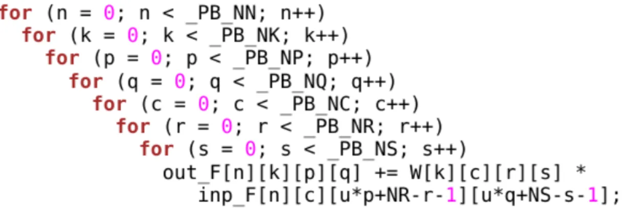
Algorithm 1Convolutional layer: Forward pass

Require: N, K, C, H, W, R, S, U, V

Require: inp[N][C][H][W]: Input data

Require: W[K][C][R][S]: Weight matrix for a given layer 1: P ←(H - R)/U + 1

2: Q←(W - S)/V + 1

3: ∀(n∈N, k∈K, p∈P, q∈Q, c∈C, r∈R, s∈S )do_{

4: out[n][k][p][q] += W[k][c][r][s] * inp[n][c][u*p+R-r-1][u*q+S-s-1] 5: }

The rest of this paper is organized as follows: In Section 1.3, we give a quick overview of poly-hedral compilation. Then, in Sections 1.4–1.7, we present the computational kernels corresponding to forward and backward phases of various deep NNs. In Sec. 1.9, we discuss the performance im-provements obtained by loop transformations. Finally, in Sec. 1.10, we state conclusions and some future work.

1.3

Polyhedral Compilation

The Polyhedral model focuses on optimizing and parallelizing the loop nests. It is a powerful for-malism to analyze and transform the input affine programs so as to run them on varieties of modern heterogeneous architectures. It can statically analyze programs which involve affine loop bounds and affine array access functions. Typically, a polyhedral compiler first creates a model of input loop nest. A statement nested within addeep loop nest is represented asd-dimensional polyhedron where each integral point represents dynamic instance of that statement. After extracting such a representation, data dependence analysis—a well studied problem that boils down to solving an integer linear programming problem [5]—is performed. This analysis finds the (dynamic) instances of two possibly different statements which access the same array location, and at least one of the accesses is a write. Such an analysis is important to preserve the semantics of original program. The second step of polyhedral compilation is the affine scheduling problem [6], that involves finding a

(16)

Deep Neural Network layers BLAS / HPC kernels

Convolutional layer Stencils, tensor multiplication

Recurrent layer Stencil with varying time steps

LSTM Set of Matrix vector products

Max, sum Pooling Max/Sum reductions

Table 1.1: Correspondance among DNN layers and HPC kernels

Table 1.2: Program Parameters for CNN

N Number of Input Images in batch C Number of Input feature maps K Number of Output feature maps P×Q Size of output feature map R×S Size of filter kernel U,V Stride parameters

complex sequence of classical loop transformations (such as loop tiling, permutation, skewing) which expose the parallelism and improve the data locality. A number of approaches exist to find a good program transformations from a large search space, and one practical approach involves scheduling two dependent statement instances as much closer (in time space) as possible. The above approach was first implemented in the Pluto source to source compiler [2] which we use in this work. The final step of polyhedral compilation involves generating a loop nest which scans all valid integer points in polyhedra [7]. The parallel loops is be marked with apt pragmas (like OpenMP, OpenACC) during code-generation.

In recent past, polyhedral compilation has shown to be effective in accelerating various linear algebra kernels, tensor contractions, stencils, image processing applications etc. We make thecrucial observation that many of the layers used in deep learning pipelines perform computations that are similar to the ones polyhedral compilation has been successful in optimizing. It is known that entries in the column 2 of above table are well optimized by polyhedral compilers. In this paper, we try to explore how polyhedral model optimizes various deep learning layers given the close correspondence as depicted in table 1.1. We also release the NN kernels. Earlier researchers who worked only on CNN [8] did not release their code (Neither HDL nor HLS/C code) to open-source. To the best of our knowledge, there is no known implementation of DNNs (as (affine) Polyhedral programs) for benchmarking purposes. With this paper we overcome the above limitation.

(17)

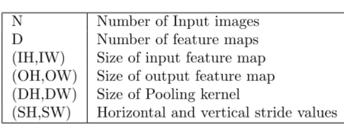
Table 1.3: Program Parameters for Pooling

N Number of Input images

D Number of feature maps

(IH,IW) Size of input feature map (OH,OW) Size of output feature map (DH,DW) Size of Pooling kernel

(SH,SW) Horizontal and vertical stride values

1.4

CNN

The program parameters of a CNN are described in Table 1.2. For parallelizing purposes, the CNN program can be thought of as a stencil (with uniform dependences) defined over a loop nest of depth seven, with the loop body computing convolution. A quick study of the dependences of the code shows that all four outer dimensions, namely n, k, p, q, are completely parallel. The array index expression for inparray accesses the appropriate location in the input feature map accounting for inverting and striding. Though our current implementation assumes absence of padding in the input filters, though it can be added at a later time. The array access is clearly non-affine (due to the

Figure 1.2: C Code : CNN backward pass

multiplication of the stride parameter with the corresponding indices). The reader is referred to Section 1.5 for a note on affinity of CNN and MaxPool. In the backward pass, the error information is propagated from output of a layer to its input. err outcontains the error derivative with respect to the output of the layer. To compute the error derivative with respect to the input, err out is multiplied with values from weight matrixW to accumulate values intoerr inmatrix.

1.5

Max Pooling

Pooling is a form of layer usually added after convolutional layer in CNN to reduce the spatial size of the representation in the network. The program parameters for max pooling operation are provided in Table 1.3. In MaxPooling, the maximum input value within the window is termed as the output of the operation as shown in Algo. 2. Only the maximum value of input window contributes to the output value. During backpropagation phase (shown in Algo. 3), the error derivative with respect to output is added only to the input pixels which have contributed to the output value.

Affinity of CNN and MaxPool: A central operation in CNN isconvolution which accesses the array index expression by multiplying thestride parameter with the loop dimension to get the required offset in the input image. Though this makes the array access function non-affine, as these

(18)

Algorithm 2Max pooling layer: Forward pass

Require: N, D, IH, IW, DH, DW, SH, SW, inp[N][D][IH][IW]: Input 1: OH←(IH - DH)/SH + 1

2: OW←(IW - DW)/SW + 1

3: ∀(n∈N, d∈D, r∈OH, c∈OW )do_{

4: val←MIN INTforeach h_∈[SH_∗r, min(SH_∗r+dh, ih))do end

w_∈[SW_∗c, min(SW _∗c+dw, iw)) 5: val←MAX(val, inp[n][d][h][w])

6: 7:

8: out[n][d][r][c]←val 9: }

Algorithm 3Max pooling layer: Backward pass

Require: N, D, IH, IW, DH, DW, SH, SW

Require: inp[N][D][IH][IW], err out[N][D][OH][OW]: Input data 1: OH←(IH - DH)/SH + 1

2: OW←(IW - DW)/SW + 1

3: ∀(n∈N, d∈D, r∈OH, c∈OW )do_{ foreach h_∈[SH_∗r, min(SH_∗r+dh, ih))do end

w_∈[SW_∗c, min(SW _∗c+dw, iw)) if out[n][d][r][c] == inp[n][d][h][w] then 4:

end

err in[n][d][h][w] += err out[n][d][r][c] 5:

6: 7: 8: }

(19)

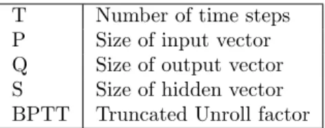
Table 1.4: Program Parameters for RNN

T Number of time steps

P Size of input vector Q Size of output vector S Size of hidden vector BPTT Truncated Unroll factor

stride parameters are constant integer literals for each individual layer within a DNN, and are fixed while designing the network, we fix them statically. A similar strategy was used by Zang et al. [8] who used Polyhedral techniques for FPGA code generation. The same argument applies MaxPool layer as well.

1.6

RNN

The unique aspect of RNNs is the feedback loop where the output of the neuron is passed as input to the same neuron leading to a recurrence in time dimension. The presence of feedback loop introduces a set of dependences during both forward and backward phases of the network. The layer has three weight matrices namely U, V, W which are learnt during propagation phase. During back-propagation, the error of output neuron is propagatedT steps back in time. The kernel parameters for a typical RNN is shown in Table 1.4.

Algorithm 4RNN layer: Forward pass

Require: BT, T, P, Q, S

Require: U[S][P], W[S][S], V[Q][S]: Weight matrices

Require: state(t), input(t): Vector of size S, P resp. 1: state(0)←U * input(0)

2: output(0)←V * state(0)foreach t∈[1, T)do 3:

end

state(t)←U * input(t) + W * state(t-1) 4: output(t)←V * state(t)

5: 6:

As described in Algo. 4, in the forward pass of RNN, state(t) denotes hidden state vector at each time step and similarly output(t) is the output at timestep t. The hidden state (state(t)) computation at time step t uses information of current input vector and hidden state vector of previous time step. U and W are multiplied with input(t) and state(t₋1) respectively and the quantities are added to get the final result. The output vector is obtained by computing an inner product ofV and current hidden state i.e. state(t).

We describe the backward pass in Algo. 5, where the error derivatives are summed up for each time step t. This computes the error accumulation of gradient using chain rule. TheerrB

S acts as

an intermediate vector during the back-propagation step to store the error derivative with respect to the hidden state vectorstate(t) represented aserrA

(20)

Algorithm 5RNN layer: Backward pass

Require: BT, T, P, Q, S, (U[S][P], W[S][S], V[Q][S]): Weights

Require: errout(t), state(t), input(t): Vector of size Q, S, P resp. foreach t∈[T−1,1]do 1:

end

errV+ =errout(t)∗state(t)

2: err_SA[1 :r] = V *errout(t)foreach step∈[t+ 1, max(0, t−BT))do 3:

end

if step >0 errW+ =errAS[1 :r]∗state(step−1) 4: errU+ =errAS[1 :r]∗input(step)

5: err_SB+ =errA_S[1 :r]∗W 6: err_SA[1 :r] =errB_S[1 :r] 7:

8: =0

Table 1.5: Program Parameters for LSTM T Number of time steps P Size of input vector Q Size of output vector S Size of hidden vector

1.7

LSTM

LSTM is a special kind of RNN, designed to combat vanishing gradients [9] through a gating mech-anism. A typical LSTM layer is comprised of a forget gate, an input gate and an output gate. Each gate masks some information (from the stream of data flowing through the network) propagating through itself, or its previous layers depending on the type of gate. The parameters required to describe LSTM are given in Table 1.5.

In Algo. 6, inputgate, f orgetgate, outputgaterepresent the input, forget and output gates

respec-tively, and work like masks. Theinputgate decides to what extent the current input contributes to

the newly computed statememory(t). Thef orgetgate, defines the factor of the previous state which

is retained in the current state. Finally, the outputgate, defines how much of the internal state is

exposed to the external network (that is, to the subsequent layers and to the next time step as well).

Algorithm 6LSTM Neural Network layer: Forward pass

Require: T, P, Q, S, (input(t), state(t)): Vectors of size P, S resp.

Require: Wi[S][S], Wf[S][S], Wo[S][S], Wg[S][S]: Weight matrices for hidden state.Suffix represent

gate type (input, forget, output, hidden)

Require: Ui[S][P],Uf[S][P],Uo[S][P],Ug[S][P]: Weight matrices for input state. foreach t∈[1, T) do

1:

end

inputgate[1:S]←input(t)*Ui+state(t-1)*Wi 2: f orgetgate[1:S]←input(t)*Uf+state(t-1)*Wf 3: outputgate[1:S]←input(t)*Uo+state(t-1)*Wo 4: candstate[1:S]←input(t)*Ug+state(t-1)*Wg

5: memory(t)←memory(t-1)*f orgetgate+candstate*input(t) 6: state(t)←memory(t)*outputgate

7:

(21)

hidden states. The method of computingcandstate is the same as that of computingstate(t) in a

RNN, except that the parameters U and W are replaced with Ug and Wg. memory(t) can be

considered as internal memory of the unit, which is a sum of two components: a) memory(t−

1) multiplied by the forget gate f orgetgate, b) newly computed candidate hidden state candstate

multiplied by the input gateinputgate. In other words, it is a combination of how we want to combine

the new input with previous memory. Given the memory(t), the output state(t) is computed by multiplying thememory(t) with the output gateoutputgate.

The back-propagation phase for LSTM(Alg. 7) consists of computing errors for vectors rep-resenting various gates(input/output/forget/cand state). Using these, errors for weight matrices are computed. Notice that, while computing errors for Ui, Ug, Uf, Uo, input(t) gets multiplied

with the error values for a gate. While, error computation of Wi, Wg, Wf, Wo requires state(t).

This is so because during forward phaseUi, Uf, Uo, Ug represents weight matrices forinput(t)and

Wi, Wf, Wo, Wg represents weight matrices for candidate hidden state.

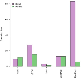
RNN _LSTM CNN SumP ool MaxP ool Ex ecution time 0 20 40 60 80 Serial Parallel

Figure 1.3: Execution times for forward pass

1.8

PolyBench/NN in Julia

Julia [10] is a high-level language suited for scientific applications. Julia code gets translated into LLVM-IR through its JIT compiler so as to facilitate varieties of compiler optimizations imple-mented in LLVM. Recently during Google Summer of Code-2016, polyhedral transformations were enabled into Julia via LLVM-Polly [11]. Hence, we also ported our PolyBench/NN programs into PolyBench.jl framework [12].

(22)

RNN _LSTM CNN SumP ool MaxP ool Speedup 0 5 10 15 0.793 1.779 2.215 1.003 14.848

Figure 1.4: Execution times for backward pass

1.9

Performance analysis

To study speedups obtained by applying polyhedral transformations, we use Pluto [2] (version 0.11.4), a widely used source-to-source polyhedral optimizer with --tile --parallel flags. All experiments were performed with the data set sizes set to the PolyBench variableEXTRA-LARGE. We compiled the parallel codes generated by Pluto using GCC-7.0.0, and OpenMP-4.5 for execution. The experiments were performed on Intel(R) Xeon(R) CPU E5-2630 [email protected] cluster having two processors with each processor having 8 hardware cores. We ran each program three times by using benchmarking script bundled within PolyBench, which internally runs it five times. We selected median of three trials as the execution time. We separately recorded the execution times for serial and parallel versions for both forward and backward phases.

Algorithm 7LSTM Backward pass

Require: T, P, Q, S, Wi[S][S], Wf[S][S], Wo[S][S], Wg[S][S], Ui[S][P], Uf[S][P], Uo[S][P], Ug[S][P],

outputgate[1:S],inputgate[1:S],f orgetgate[1:S],candstate[1:S]

Require: memory(t), input(t) Vector of size S, P respforeach t∈[T−1,1)do

1:

end

errg_output= memory(t)*errstate(t)

2: errmemory(t)+=outputgate[1:S]*errstate(t)

3: err_{f orget}g = memory(t-1)*errmemory(t)

4: errmemory(t−1)+=f orgetgate[1:S] *errmemory(t)

5: err_inputg =candstate[1:S] *errmemory(t)

6: err_{cand state}g =inputgate[1:S] *errmemory(t)

7: err Ui/g/f /o+=input(t)*(errg_{input/cand state/f orget/output}) 8: err Wi/g/f /o+=state(t)*(err

g

input/cand state/f orget/output)

9: errstate(t−1)+=Wi*errinputg +Wf*errg_{f orget}+Wo*erroutputg +Wg*errg_{cand state} 10:

(23)

RNN _LSTM CNN SumP ool MaxP ool Ex ecution time 0 200 400 600 800 Serial Parallel

RNN _LSTM CNN SumP ool MaxP ool Speedup 0 10 20 30 40 50 1.713 1.596 51.783 0.371

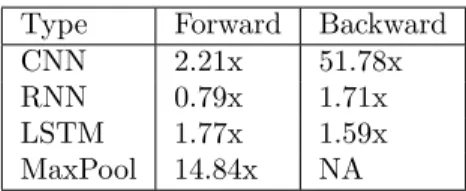
The plots showing execution times for forward and backward phases are given in 1.3 and 1.6 respectively. We make following observations from plots: 1) Backward phase is more compute intensive than forward phase for all layers except SumPooling. 2) RNN, LSTM consist of Polyhedral loops that are successfully parallelized by Pluto. 3) For CNN and Maxpool, we were forced to replace the stride parameters with integer constants defined in our header file. This made CNN and Maxpool (forward pass) analyzable for Pluto. 4) The backward phase of MaxPooling kernel

(24)

Type Forward Backward

CNN 2.21x 51.78x

RNN 0.79x 1.71x

LSTM 1.77x 1.59x

MaxPool 14.84x NA

Table 1.6: Speed-up over serial execution

consists of a data dependent condition which Pluto's dependence analysis is unable to analyze. 5) No speedups were observed for forward phase of RNN and backward phase of SumPooling. 6) Average speedups observed for forward and backward phases are 2.15 and 2.69 respectively.

1.10

Conclusions And Future Work

We implemented the four varieties of neural network layers as loop-programs in the PolyBench framework. While RNN and LSTM strictly adhere to Polyhedral framework’s affinity conditions, CNN and MaxPool do not and we had to fix the stride parameters of their codes manually. The programs show significant speedups after applying polyhedral transformations. We released our PolyBench/NN C implementation https://github.com/hrishikeshv/polybench/tree/master/ polyNN so that other researchers can work on advanced optimizations on these kernels. Though our work is preliminary, we believe it will form a basis to apply automatic loop transformations that expose parallelization as well as data locality optimization opportunities for different DNN architectures on various heterogeneous architectures and accelerators.

(25)

Chapter 2

Exploiting GPU caches by

Polyhedral compilation

e propose a compiler driven method by which parallel computations can be accelerated on GPUs by exploiting the various special varieties of caches (such as texture, surface and constant for NVIDIA GPUs) available on them. We show that our method obtains superior performance, when compared with earlier methods of accelerating these classes of computations that use on-chip shared memory. We provide an end-to-end solution by developing a fully automatic framework within a state-of-art source-to-source Polyhedral compiler (PPCG) to exploit these varieties of GPU caches. Using techniques from the formalism that Polyhedral model provides, we reason about the profitability of using each of the particular variety of GPU caches. We evaluate our implementation on kernels from PolyBench/C benchmark and reportup to 1.5x speedups over the existing memory mapping strategy used by PPCG compiler. As the usage of particular variety of cache is highly application specific, we also consider five representative computations namely: PageRank, Recurrent Neural Network, Long Short Term Memory layer, Poisson Solver and DWE-FDTD stencil and show that usage of special GPU caches in these programs results in up to 2.6x speedup over a standard shared memory based implementation. With these use cases, we show the general purpose computing usage of these special GPU caches that were originally designed for image processing applications. With increasing interest in mapping general purpose algorithms on GPUs, we believe that our contribution is towards automatic exploitation of GPU cache/memory hierarchy.

(26)

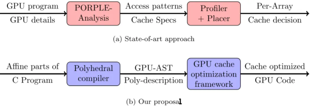
PORPLE-Analysis GPU program GPU details Profiler + Placer Access patterns Cache Specs Per-Array Cache decision (a) State-of-art approach

Polyhedral compiler GPU cache optimization framework Cache optimized GPU Code GPU-AST Poly-description Affine parts of C Program (b) Our proposal

Figure 2.1: Profiler based approaches employ less-precise analytical models to guide cache decisions. We use polyhedral representation to precisely model profitability criterion as specified by GPU vendors thereby resulting into end-to-end fully automatic framework.

2.1

Introduction

The advancements made from the traditional processor architecture to multi-core, many-core ma-chines after the collapse of Moore's law are greatly improving the execution times of various applica-tions. Also, special hardware accelerators like GPUs are being used to speedup highly parallel SIMD programs. However, it is well understood that correctly programming such parallel accelerators is not only difficult but also highly error prone. Ever since the beginning of compilers, optimizing compilers have long been shown themselves to be effective in making programmers free of the chal-lenges involved in writing correct and efficient parallel programs. The primary motivation for many of the optimizing compilers is to design new optimization strategies so as to expose and exploit the parallelism present in the input program.

Such an approach of auto-parallelization has multiple benefits. Firstly, by relying on static/dy-namic analysis implemented within the compiler, the correctness of the transformed program can be guaranteed, as long as the compiler is free of bugs. Secondly, supporting upcoming architectures reduces to the problem of writing a new backend, which is a well understood engineering challenge. Finally, and most importantly, with extra target-specific information, the compiler can exploit the available hardware resources to the maximum possible extent.

It is this last benefit that our work focuses on: by performing rigorous static and dynamic analyses, optimizing compilers can generate efficient parallel/vector programs that can exploit the complete power of multi/many core machines along with their hardware intricacies.

Polyhedral model is a powerful formalism to automatically parallelize the affine programs. In recent past, using polyhedral model, many tools have been developed to optimize programs for CPUs and various accelerators. PPCG [13] is one such state-of-art polyhedral compiler that analyzes affine parts of programs written in C, and automatically generates CUDA/OpenCL code, while incorporating several GPU specific transformations.

Parallelizing and optimizing compilers employ a variety of affine transformations to effectively utilize the memory hierarchy with multiple level of caches. For CPUs, such transformations result in effective utilization of on-chip L1, L2 and shared L3 level caches. In case of GPUs, the situation is a little different; large number of cores share common GPU global memory. As GPU global memory has much higher access latency [14], effective utilization of global memory bandwidth by reducing the global memory accesses is critical to accelerate computations on GPUs. Thanks to architecture level advancements, GPU architectures support a variety of software managed caches. These include

(27)

shared memory (software managed portion of L1 cache),constant cache, texture cache andsurface

cache (Table 2.2).1 _{Beyond software managed caches, GPU architectures also support large register}

files, and fast on-chip L1 and L2 level caches.

With this work, we make a case that, for real world computations that can be mapped to GPUs, exploitation of shared memory incurs extra overhead. This can be avoided by effectively utilizing special varieties of GPU caches, namely, surface/texture/constant memory in NVIDIA GPUs and image/constant memory in AMD GPUs.2 _{Thereby, we show the} _{general purpose computing usage}

of these special GPU caches that were originally designed for image processing applications.

2.2

A Motivating Example: LSTM layer

For real-world computations in general, GPU shared memory may not be a good choice to access arrays. To substantiate this claim, consider the computational kernel shown in Fig. 2.2. This kernel depicts the working of forget gate included in Long short term Memory layer. LSTM layer is widely used by deep learning community for various learning tasks in Natural language processing (NLP). Even though we show only one portion of the LSTM code (representing forget gate only), discussion is applicable to other types of gates involved in LSTM layer (such as input gate, output gate). In LSTM, the outermost (time) loop captures the context information. At every time step, the kernel computes the vector f by simply taking weighted combination of (i) input at current time step

inp F[t], and (ii) context provided by previous time step(s F[t-1][...]). In the above Figure, theU_f, W_farrays correspond to the weight matrices learned by the LSTM layer during training phase. Finally, vectorfdepicts the output for the forget gate of LSTM layer at given time stept.

At each time step, the kernel simply performs sequence of array-multiplication followed by a

reduction operation with sum as operator. It can however be noticed that the above computation uses a large number of arrays. Thanks to the affine nature of the above computation (affine array access functions, affine loop bounds), GPU code can be generated for it by using the PPCG compiler. PPCG employs a variety of analyses and transformations on the input program to effectively manage data in the register files, perform array privatization, exploit shared memory by performing array reuse analysis, and optimize the data transfers from CPU to GPU global memory. The relevant sections of the output produced by PPCG is shown in Figure 2.2.

Table 2.1: Execution times of PPCG generated CUDA code for LSTM layer on NVIDIA GPUs (Problem size: T=400, S=2850, P=3000)

PPCG:Global PPCG:Shared PPCG:Caches

Tesla K20X 9.504 sec 3.882 sec 1.785 sec

Tesla P100 2.434 sec 1.968 sec 1.429 sec

In the transformed program, the GPU kernelkernelis invoked for each iteration of a sequential

loop (with iterator c0) which essentially executes on the host (CPU). Also, the GPU kernel uses low-latency shared (also termed as scratchpad) memory and therefore, achieves good amount of

1_{GPU programming literature refers texture/surface/constant as memories rather caches.} _{This is because, as}

per GPU programming APIs, these are treated as objects which encapsulates the program data (arrays) that are supposed to be accessed through special varieties of caches. The special caching techniques allow to access these objects effectively.

2_{Though our framework equally applies to special caches available on both NVIDIA and AMD GPUs, our code}

(28)

Figure 2.2: LSTM: Original C-code fragment and PPCG Generated CUDA Code 1 f o r ( t = 0 ; t < PB T ; t++) 2 f o r( s 1 = 0 ; s 1 < PB S ; s 1++) _{ 3 f [ s 1 ] = 0 . 0 ; 4 f o r( p = 0 ; p < PB P ; p++) 5 f [ s 1 ] += U f [ s 1 ] [ p ] ∗ i np F [ t ] [ p ] ; 6 i f( t > 0 ) 7 f o r( s 2 = 0 ; s 2 < PB S ; s 2++) 8 f [ s 1 ] += W f [ s 1 ] [ s 2 ] ∗ s F [ t 1 ] [ s 2 ] ; 9 } 1 g l o b a l void k e r n e l ( . . . )_{ 2 . . . 3 s h a r e d f [ . . ] = f [ . . ] ; 4 s h a r e d U f [ . . ] [ . . ] = U f [ . . ] [ . . ] ; 5 s h a r e d i n p F [ . . ] [ . . ] = inp F [ . . ] [ . . ] ; 6 s y n c t h r e a d s ( ) ; 7 f o r (i n t c4 = 0 ; c4 <= ppcg min ( 3 1 , c2 + 2 9 9 9 ) ; c4 += 1 ) 8 s h a r e d f [ t 0 ] += ( s h a r e d U f [ t 0 ] [ c4 ] ∗ s h a r e d i n p F [ 0 ] [ c4 ] ) ; 9 s y n c t h r e a d s ( ) ; 10 f [ . . ] = s h a r e d f [ . . ] ; 11 } 12 } 13 h o s t void LSTM layer ( . . . )_{ 14 . . .

15 // Copy d a t a from CPU t o GPU

16 f o r (i n t c0 = 0 ; c0 <= 4 0 0 ; c0 += 1 )_{ 17 dim3 dimBlock ( 3 2 ) , dimGrid ( 6 3 ) ;

18 k e r n e l <<<dimGrid , dimBlock>>> ( . . . ) ; 19 // s y n c h r o n i z e and l a u n c h o t h e r k e r n e l s 20 _} 21 // Launch n e x t k e r n e l 22 . . . 23 }

(29)

speedup over the original na¨ıve global memory based implementation. But, the following crucial

observations can be made on these programs:

1. Arrays U_f, s_F, W_f, inp_F are read-only; both in the original, as well as the transformed program.

2. Before starting computations within a GPU kernel, small portion of arrays need to be copied from global memory to the shared memory. Note that this need to happen for each iteration of the outer-loop executing on hostc0.

3. All the threads within acudablockmust synchronize once the data has been loaded to shared memory. This contributes to extra latency; again, this is incurred for each iteration of outer-loopc0.

So, in the above computation, read-only texture cache3_{is an apt choice for accessing arrays U˙f,}

W˙f. Using texture cache eliminates each of the latencies mentioned in observations 2 and 3, and therefore results in superior performance. All these observations create a motivation for having a unified automatic framework to support the entire GPU cache/memory hierarchy.

Contributions: We make the following contributions:

• We show theoretically as well as empirically the limitations of usage of shared memory on real-world kernels of iterative nature. As a solution, we design a compile-time, fully automatic GPU cache exploitation framework in the state-of-art source-to-source polyhedral compiler. Our framework supports all GPU caches, including surface caches, an architectural advancement of texture caches.

• We design a sound (on weaker memory models) static analysis to ensure program correctness after transformation. We formalize the profitability guidelines provided by GPU-vendors (like NVIDIA) for varieties of caches using integer set arithmetic and integer linear programming.

• On the PolyBench/C benchmarks we reportup to 1.5x speedupsover existing PPCG. As the speedups after cache exploitation vary from program to program, we show that our framework can accelerate some additional (representative) real-world iterative computations: PageRank, RNN, LSTM, PoissonSolver and FDTD kernels. On these important programs from different domains, we show up to 2.6x performance improvements over auto-generated codes (using PPCG) that useshared memory, and up to 1.27x over manually annotated codes (using PGI). We thereby show that GPU special caches could be effectively used in domains beyond than what they were originally designed for.

• Considering that PPCG already exploits local, shared, and global memory effectively, with our new framework added into PPCG, it is now able to support the complete GPU cache and memory hierarchy automatically. To the best of our knowledge, none of the existing (fully/semi) automatic optimizing compilers support code-generation for the complete GPU cache/memory hierarchy.

(30)

The remaining part of this section is organized as follows: First, in Sec. 2.3, we summarize the related work. In Sec. 2.4, we introduce polyhedral model and the PPCG compiler. In Sec. 2.5, we discuss GPU memory hierarchy with a focus on special caches. In Sec. 2.6, we discuss static analysis and cache decision algorithms. In Sec. 2.7, we describe the cost model, while in Sec. 2.8, we discuss code-generation. In Sec. 2.9, we describe the evaluation results on PolyBench/C suite. In Sec. 2.10, we show how our framework accelerates some real-world kernels (PageRank, RNN, LSTM, PoissonSolver, FDTD) and finally in Sec. 2.11, we state conclusions and future work.

2.3

Related Work

There has been a significant work on automatic and semi-automatic compilation strategies to map general purpose and affine programs on GPUs. The polyhedral model has been successful in effec-tively parallelizing the sequential programs for GPUs. One such first experimental prototype tool namely CToCUDA-C was by Baskaran et al. [15, 16] and uses PLUTO compiler to obtain program transformations; while it claims to support constant memory, we were unable to obtain constant memory optimized CUDA code for some simple kernels. The tool does not support texture caches. (We used pluto-0.6.2-cuda [17].)

LLVM/Polly-ACC [18] supports PTX code generation from LLVM/Polly [19], but lacks support for GPU caches. R-Stream [20] a proprietary compiler from Reservoir Labs that uses polyhedral framework to map SCoPs to GPUs. Due to its unavailability, we could not use it for any comparison; their paper [20] does not discuss about GPU caches.

While our framework is fully-automatic, there are many semi-automatic approaches where the user can specify the affine transformations to the compiler to generate parallel code. CUDA-Chill [21] is an example; it lacks support for GPU caches. PGI compiler from Portland group and NVIDIA accepts C/Fortran programs with OpenACC annotations for loops and array-annotations (only for texture/constant and not surface caches) that are interpreted by the compiler to generate PTX code. Even among PGI compilers, texture/constant cache support seems to be limited to the PGI CUDA Fortran compiler [22].

Another popular semi-automatic tool OpenMPC [23] is developed on the top of Cetus infrastruc-ture which extends OpenMP so that the user can provide annotations. Like in the PGI compiler, OpenMPC allows annotations to access arrays, but that too only from texture caches.

2.4

Polyhedral Model and PPCG

The Polyhedral model works on compute-intensive parts of a program and hence targets loop nests. The specific variety of loops that Polyhedral Model operates on are called Static-Control Parts of program (SCoP). Essentially, SCoPs are statically analyzable because of usage of affine-expressions for loop bounds, conditionals, array accesses. Polyhedral model represents statements nested within a d-deep loop nest as a d-dimensional polyhedron in the Euclidean space, henceforth referenced as iteration domain. A valid integer point inside the iteration domain corresponds to a dynamic instance of that statement. In the polyhedral model, array data-flow analysis [5, 24] is performed to detect two dynamic instances of statements, both of which access the same array element, and at least one of them is write. In order to preserve program semantics, dependences are used to obtain

(31)

Table 2.2: GPU cache varieties GPU vendor Variety of Cache Optimized for spatial access Optimized for broadcast access NVIDIA Texture (Read only)

Surface (Read + Write) Constant (Read only)

AMD Image (Read + Write) Constant (Read only)

constraints on coefficients of the statement wise transformation matrices, thanks to affine form of Farkas lemma [6, 24]. By the procedure, an affine transformation search space is obtained, where each (integral) point represents a valid program restructuring [25]. Of the several approaches of scheduling, the approach by PLUTO [2] has been shown to be practical as it gives a transformation with maximum permutable schedule dimensions. This makes loop tiling legal over permutable band of the schedule. Finally, the original program that is modelled as a union of polyhedra and a schedule (a bijective map from original space to transformed space) are given as input to code generation algorithm [7] which generates the loop nests that scan the transformed union of polyhedra. Parallel schedule dimensions can be detected and marked asdoallloops.

PPCG PPCG is an open-source C to CUDA-C/OpenCL automatic parallelizer based on poly-hedral model. PPCG detects SCoPs from input C programs using Polypoly-hedral Extraction Tool (PET) [26]. PPCG performs dependence analysis by using Integer Set Library (ISL) [27], a li-brary for manipulating integer sets bounded by affine constraints. ISL supports algorithms useful in analyzing and transforming SCoPs, like Feautrier's dependence analysis [5].

To compute a schedule, PPCG uses the ISL scheduler—a variation of PLUTO's algorithm [2]— which allows to set several options so as to tailor the scheduling process. PPCG finds a schedule by maximizing permutable dimensions. PPCG generates GPU code only if each permutable band present in the schedule contains at least one parallel schedule dimension. This allows to generate GPU code for each permutable band by tiling it. Since GPU architectures support two levels of parallelism (block and thread level), outermost parallel dimensions within each permutable band are tiled to support these two levels of parallelism. The tile loops are then mapped to blocks, and the point loops are mapped to threads. Based upon the number of parallel schedule dimensions in each band, PPCG generates 2D or 3D kernel grids and thread blocks. PPCG uses ISL-AST code generator [28] to obtain kernel AST. The generated ISL-AST is transformed into CUDA or OpenCL kernel function. PPCG also generates corresponding host code.

PPCG supports some GPU specific optimizations of which, the prominent are: (1) Array lin-earization: To enable coalesced access to GPU global memory. (2) Array privatization: Avoid accessing global memory by promoting arrays to scalars. (3)Usage of shared memory: By creating a small tile of the array and storing that tile in shared memory.

2.5

GPUs: Memory Hierarchy

As per Flynn's taxonomy, GPUs comes under the SIMD category. A GPU architecture involves collection of streaming multiprocessors (SMs) each having 32 cores. A GPU application is executed by launching large number of threads. All the threads are grouped into fixed sized (user-specified) blocks. Each block is scheduled to execute on some SM. SM scheduler selects consecutive 32 threads

(32)

(termed as a warp) from a block and executes it in SIMD fashion. GPUs hide memory latency, pipeline stalls by switching to ready-warps.

A GPU architecture comprises of DRAM where all the address spaces are mapped. By default, all the program arrays are stored in global memory space. GPU supports a low latency, software managed shared memory which is essentially a part of L1 cache. GPUs typically support large register files (to store private variables) facilitating parallel access by threads. Also, in order to optimize accesses to read only data, GPUs support a special type of cache, namelyconstantcache. Historically, GPUs were used for accelerating image/video processing applications andtexturecache was designed to accelerate such applications. Texture cache is supported by a sophisticated caching hardware: texturizing hardware. Considering the topic of this section, we discuss these special caches in detail.

Constant Cache: The constant cache is additional to, and physically different from regular on-chip L1, L2 level caches. It is optimized for read-only broadcast access patterns, and is useful in cases when all the threads within a warp need the same (read-only) data. For applications involving large number of arrays, accessing the suitable arrays through constant cache helps to improve the utilization of L1, L2 level caches.

Texture and Surface caches: The Texture/Surface caches are specially designed for spatial array access patterns. While accessing 2-D or 3-D arrays4 _{using texture/surface caches, the array}

linearization is done in a way that preserves the spatial neighborhood of array elements, as it would be in 2-D or 3-D space respectively. By doing so, when a particular array element is accessed, its spatial neighbor elements arecached. In contrast, for normal caches, linearizing 2-D or 3-D arrays (by row-major, or column-major order) destroys the spatial neighbourhood.

This special type of array flattening—linearization which preserves spatial neighbourhood—is typically achieved by using space-filling curves (mainly Z-curves). The uniqueness of Z-curves lies inside their simplicity of interpolation function that is required for address translation mechanism. The interpolation for Z-curves involves application of bitwise operations (likeand and shift), that can be implemented as a hardware circuits, thereby making address translation mechanism to be hardwired. It is clear that for a normal L1/L2 level cache to take care of such special types of array flattening, it would have to be supported by sophisticated cache mapping techniques along with an address translation mechanism. Hakura et al. [29] and Doggett et al. [30] discuss these techniques in detail.

When to use Texture/Surface Caches? Texture/surface caches are promising for array accesses patterns that exhibit spatial locality, like, in case a program accesses both B[i][j-1] and B[i-1][j] values. Then, no matter how array flattening is done (row/column major order), it is very likely that at least one cache miss will occur.5 _{In case, if any other thread within the same warp}

also accesses one of those two locations, then one global memory access gets saved.

2.5.1

Read-Write incoherency

Texture cache only supports read-only arrays. The workaround to access writable arrays via texture cache is as follows: create two copies of the array with one copy residing on texture cache while other on global memory. All the reads from that array can be altered programmatically so as to

4_{Note that array dimensionality should be strictly less than 4 so as to access it through texture/surface caches.} 5_{A subtle assumption here is that: array A is large enough, and no data locality transformations are applied.}

(33)

access from the copy residing on texture cache. All the writes to that array must be performed to the copy residing on global memory. However, this is guaranteed to work only if the update (written) array value is not read by any of the thread inside a kernel. This is because the updated value resides on the global memory array copy and array is read from the copy bound to texture cache. This is termed asRead-Write incoherency and should be avoided to ensure correct semantics. The workaround also suffers with a limitation of requiring two copies of array; increasing memory footprint of the application. To eliminate this limitation, NVIDIA GPU architectures starting from Fermi (with Compute capability ¿= 2.0) support a writable variant of texture cache, namely surface cache. We note that read write incoherence should be avoided to ensure correct semantics if program uses surface cache.

Polyhedral Extraction

Tool

C Program _Dependence Analysis

PET Tree Affine

scheduling Dependences Polyhedral AST generation Schedule Static analysis Kernel-AST Cache decision algorithm Valid candidate arrays Cost model Cache decision for each array

Kernel AST alteration Refined decision for each array Host AST alteration Host-AST PPCG Code generation Kernel-AST Host-AST

Cache optimized CUDA code

Figure 2.3: Overview of our Framework

(Colour Encoding: Red≡PPCG module, Blue≡Proposed module, Green≡Modified PPCG module.)

2.6

Automatic Framework for Cache Exploitation

In this section, we describe our automatic cache exploitation framework. By default, we assume that the surface cache is supported. We also exposed the -no-surface-memory flag so as to have flexibility and backward compatibility for target GPUs having compute capability ¡ 2.

Our schema is explained in Figure 2.3. First we allow PPCG to analyze, transform the input program. Once PPCG generates the AST, our algorithm performs static analysis so as to ensure that Read-Write incoherency is avoided. We discard the arrays which result in incoherency and access them using global memory. Then, we use the cost model to reason about profitability of accessing an array via candidate GPU caches. After making the appropriate cache decision for each array, we alter the kernel-AST and host-AST.

(34)

None start Read Write LRead Invalid W !L&R L&R L&R !L&R W R W W&L R&L W&!L R&!L R,W W:Write access R:Read access L:Access inside loop/s

Figure 2.4: Automata showing transitions of new state

2.6.1

Static Analysis

In order to preserve semantics, arrays resulting in read-write incoherence must be discarded from candidate list of surface cache. In other words, during kernel execution, updated array value (by any of the thread within a kernel) must not be read (by same or other thread). Since, GPU programs are Single Instructions Multiple Data (SIMD), it suffices to make sure that for a given array, kernel-AST is free of write followed by Read access (W-R access sequence) for a candidate array. Notice that, the analysis is conservative in the sense that information about accessed location is discarded. Our analysis traverses the entire GPU-AST visiting kernel statements, and detects potential W-R access sequence for all the arrays in the program. A subtle point while traversing tree is that children of a node must be processed in right to left order. This ensures correct analysis for assignment statements of following form: where A is free from read-write incoherence: A[i] = A[i] + b[i]

Another small caveat in static analysis is that, if a loop contains Read followed by Write access (R-W sequence) for some array, then it is likely to cause R-W incoherency. Because of implicit back-edge for a loop, (R-W) sequence embedded within a loop can effectively be: R-W-R -W-R-W,.... Hence, static analysis must look for R-W sequence as well; when array access is surrounded within a loop nest. If the transformed-AST comprises of if-else constructs, we analyze each branch separately and perform a conservative analysis. This means, presence of R-W incoherence in either of the branches implies presence of R-W incoherence in the entire if-else construct. A pseudo-code which performs static analysis is summarized in Algorithm 1. The corresponding automata which decides hownew stategets computed is shown in Figure 2.4.

The surface cache is refreshed each time a new kernel is launched [31]; thereby, values updated by the previous kernel would be read in the next kernel launch while preserving coherency. Therefore, we do not need to look for W-R incoherence across kernels. Hence, we force all the candidate arrays inNONE state before analyzing next kernel.

We note that detecting read only arrays for a sequence of GPU kernels (which are extracted from a single SCoP) turns out to be a special case of static analysis. The arrays accepted viaRead

or LReadstate of the automata are guaranteed to be read only arrays. We consider such arrays as candidates for texture and constant cache.

(35)

Completeness

The input program to PPCG is affine. Polyhedral transformations are essentially iteration reordering transformations. Hence transformed AST also has regular control flow involving only loops, if-else constructs, statements. Our static analysis considers all of these constructs.

Soundness

Our static analysis assumes relative ordering among memory access is same as in program text. However, due to architecture level optimizations (such as load/store buffering), such ordering may not necessarily get respected at runtime. This is especially true in case of weaker memory models. It has been experimentally observed by Algave et al. [32] that GPU memory models are believed to have weaker memory models.6

1 2 d e v i c e k e r n e l ( . . . ) _{ 3 i n t i = t h r e a d I d x . x + blockDim . x∗b l o c k I d x . x 4 B [ i ] = A[ i ] + A[ i +1] + A[ i + 2 ] ; 5 _} 6 . v i s i b l e . e n t r y k e r n e l ( . . . ) { 7 . . . 8 s u l d {\%r 2 8}, [ s u r f R e f A ,{. . .}] ; // Read S u r f a c e v a l u e s 9 s u l d _{\%r 2 9_}, [ s u r f R e f A ,_{. . ._}] ; 10 s u l d _{\%r 3 1_}, [ s u r f R e f A ,_{. . ._}] ; 11 . . . 12 mul . f 3 2 _\%r42 , _\%r29 , 0f3E4CCCCD ; // c o m p u t a t i o n s 13 . . . 14 s u s t [ s u r f R e f B , _{. . ._}] , _{\%r 4 2_}; // Write S u r f a c e v a l u e s 15 _}

Listing 2.1: Sample kernel and PTX assembly after using surface cache. Due to intermediate computations, reads are guaranteed to finish before initiating surface writes; thereby making memory view consistent.

We make the important observation to ensure the validity of static analysis at run-time even on weaker memory models. Every GPU kernel generated by PPCG is free of data-races due to exact data-dependence analysis. Hence, there are no observers (read/write from other threads) for a memory location written by a particular thread. Single thread always has a consistent view of memory. In spite of the above observations, two memory accesses (to different addresses) within a thread might get reordered (because of architectural latencies). Due to such re-ordering, it may appear that static analysis may get invalidated at execution time. 7 _{However, we make the following}

argument to rule out such possibility: (1) Arrays accessed through texture and constant caches are read-only, and notice that re-ordering of two read-accesses does not invalidate the static analysis during execution time. (2) For surface caches, our static analysis rejects candidate array with W-R

6_{Exact characterization of memory consistency model needs accurate architecture details (eg memory latency) that}

are not revealed by GPU vendors.

(36)

access sequence. Furthermore, write only arrays are not good candidates for surface cache because surface cache is a writable variant of read-only texture cache. This implies that the candidate array is guaranteed to be accessed only by R-W access sequence within a kernel. At the start of the kernel, all the threads read required values from reference bound to surface cache, then perform computation, and finally at the end of the kernel writes values through the reference. Observe that surface reads must be completed before starting the actual computations otherwise it leads to incorrect results. Also, newly computed values will be written to surface cache implying writes must be initiated after computations. Transitively, we can infer that surface reads are guaranteed to be finished before starting surface writes thereby making static analysis valid (Refer 2.1). Finally, reordering of surface-reads (correspondingly surface-writes) among themselves still makes the static analysis to be true at run-time. Even though our static analysis might appear to be designed considering a sequential consistency of memory operations, it is sound for weaker memory models (like GPUs) due to specialty in access pattern.

2.6.2

Cache selection

Static analysis aids in analyzing the candidate arrays, so that semantics are preserved even after accessing each candidate array through appropriate caches. For cache selection, first we analytically decide potential caches, then we query cost model (discussed in the next section) for profitability checks. The analytical cache decision tree 2.7 decides potential caches for arrays. The decision is made at per-SCoP granularity. This avoids array setup time in-between two successive kernel launches which are extracted from the same SCoP. Depending upon no-surface-memory flag,

al-gorithm decides whether to use surface cache or not. Read only arrays are candidates for texture, constant cache. Algorithm chooses global memory for: (1) Candidate arrays end-up being in invalid state (2) Write-only arrays.

Given Array A ∃kernel k state(k,A) =invalid? Global Is A Read-only? Texture or Constant Compute capability <2? Surface Global Yes No Yes No Yes No

Figure 2.5: GPU-cache decision tree

2.7

Cost Model

In this section, we use the power of polyhedral framework to design a cost model for each variety of cache. We analyze each array access present in the kernel and reason about its profitability.

(37)

(a) Constant cache (b) Texture cache Figure 2.6: Profitable access pattern for a 2-D array

In the polyhedral model, array accesses are modelled as a functions from iteration domain(I) to array access location(L). Formally, Foriginal : I → L. Transformed array access function for

ar-ray A is derived using original access function and newly computed schedule (Ftransf ormed(A) =

Foriginal(A)◦schedule−1). Our cost model analyzes transformed array access functions for all

can-didate arrays. For notational convenience, we assume Ftransf ormed(A) denotes transformed array

access functions for all the references to arrayA.

2.7.1

Cost model for Constant cache

Constant cache is well suited if all the threads within a same warp access the same memory element. In other words, the array access expression should be independent of thread identifiers (threadIdx.x,

threadIdx.y, threadIdx.z). Recall that PPCG maps tile loops to blocks, and point loops to

threads. Therefore, array access function should be free from the point loop iterators(iterpoint)

[Fig. 2.6]. Formally, for a candidate array A, if following formula evaluates toTrue, we decide to access it using constant cache.

^

a∈Ftransf ormed(A)

^

p∈iterpoint

a.isIndependent(p) _(2.1)

2.7.2

Unified Cost Model for Texture/ Surface caches

Recall that usage of texture and surface cache is profitable if threads within a same warp access neighbouring locations in 2-D or 3-D data space (See Fig. 2.6). Our cost model captures this situation by operating over integer sets.

We assume the following notation: letAbe the array to be analyzed andnbe the dimensionality ofA. Recall that 1¡=n¡=3. Letf be function with which arrayAis accessed for some statementS

present in GPU kernel AST. LetI be the transformed iteration domain for statementS.

First we construct a setD which captures the neighbouring elements of ArrayA. SinceD⊂A, it follows dim(D) = dim(A). We construct universal set of dimensionn. Then for each dimension

d∈D we add a constraint of form: 0<=d <= 2. Operating on parametric integer sets leads to un-scalability. Since we need to analyze every candidate array access appearing in the transformed program, we purposefully fix the starting location of setD within arrayA. Such a design allows to efficiently estimate (as opposed to exact calculation of) the spatial locality. Next, we compute the setT _⊂Iwhich comprises of iterations accessing the elements in setD. We use pre-image operation to computeT.

(38)

x y z Spatial array neighbourhood as integer set

Subset(in red) of iteration space accessing spatial neighbourhood

Only retain dimensions mapped to cuda-blocks

Linearize the space to check whether iterations belong to the same warp

(length of set<= 32)

PreImage Projection Image

Figure 2.7: Statically modelling spatial access pattern within a GPU-warp through polyhedral operations Note that, T may include following types of loop dimensions.(1) Outer loop dimensions which corresponds to loops mapped to host code.(2) Block dimensions corresponds to the loops mapped to blocks (3) Thread dimensions represents loops mapped to threads.(4)Inner loop dimensions repre-sents the loops appearing within a thread. We are interested in estimating spatial locality available within a warp. Hence, we project out the all but loop dimensions which are mapped to threads.

T0₌_{P roject out}₍_{T, dim}

outer, diminner, dimblock)

GPU architectures supports upto 3 thread dimensions (threadIdx.x, threadIdx.y, threadIdx.z). Hence, dim(T0_{) ¡=3. GPU runtime linearizes 2-D or 3-D thread dimensions [31] by using following}

mapping whereBx,By represents the kernel block dimensions.

L:tlinearized=tx+ty∗Bx+tz∗Bx∗By

PPCG uses tile sizes as kernel block dimensions. We use tile sizes in place of Bx and By. We

refer to this function as linearization mapL. UsingLwe can linearizeT0_{to obtain 1-D set}_W_.

W =Image(L, T0₎

W exactly captures the linearized iterations that access neighbouring elements in array A. We can compute length ofW as follows:

Wlength=lexmax(W)−lexmin(W)

Observe that computing Wlength involves solving two integer linear programming problems.

Wlength can be interpreted as fictitious warp size which accesses neighbouring elements in Array

Athrough given access functionsf. For each arrayAwe compute average fictitious warp sizeWavg

by computing average ofWlength computed for each access function f. In ideal case Wavg should

be close to (or less than) 32 (actual warp size on GPUs). Due to thread linearization, it may not necessarily be the case. In order to make a decision on whether to use texture or surface cache we use criterion shown in table 2.3

Spatial locality for 1-D array is implicitly captured by normal (L1, L2 level) caches. Therefore cost model refuses to access such arrays from texture/ surface cache. The upper bounding threshold value forWavgfor texture cache is set to twice of actual warp size on GPU. While for surface cache,

(39)

Table 2.3: Profitability parameters for texture, surface caches Cache/ Memory choice Metrics of profitability Array accesses Estimate of spatial locality (W {avg}) Array Dimension

Global Write-Only W avg>=65 1-D

Texture Read-Only W avg<= 64 2-D/3-D

Surface Read+Write 5<W avg<= 50 2-D/3-D

upper bound forWavgis set to 1.5 times of actual warp size. We empirically observed that usage of

surface cache introdu