Analysis of standing sound waves using holographic interferometry

Analysis of standing sound waves using holographic interferometry

Daniel A. Russell,a兲David E. Parker, and Russell S. Hughesb兲

Department of Physics, Kettering University, Flint, Michigan 48504

共Received 5 December 2008; accepted 12 May 2009兲

Optical holographic interferometry was used to study standing sound waves in air inside a resonance tube driven by a small loudspeaker at one end. The front face of the resonance tube was constructed with plexiglass, allowing optical interrogation of the tube interior. The object beam of the holographic setup was directed through the plexiglass and reflected off the back wall of the resonator. When driven at resonance, the fluctuations in the air density at the antinodes altered the refractive index of the air in the tube, causing interference patterns in the resulting holographic images. Real-time holography was used to determine resonance frequencies and to measure the wavelengths of the standing waves. Time-average holography was used to observe the effect of increasing the sound pressure level on the resulting fringe pattern. A simple theory was developed to successfully predict the fringe pattern. ©2009 American Association of Physics Teachers.

关DOI: 10.1119/1.3147683兴 I. INTRODUCTION

More than 40 years ago Powell and Stetson1,2 described

time-average and real-time3techniques of holographic inter-ferometry and their usefulness in analyzing the steady state vibration of small objects. Since then, time-average holo-graphic interferograms have become useful tools for the vi-brational analysis of musical instruments,4–6 and double ex-posure holographic interferometry has been used to analyze transient vibrations7as well as liquid diffusion8and air flow.9 The accessibility of holographic interferometry in the under-graduate laboratory has been demonstrated by several papers.10–13

Salant et al.14 demonstrated that a transparent standing

sound wave with sufficient amplitude in air can produce fringes on a time-average holographic image. More recently, Peterson et al.15 used stroboscopic holographic interferom-etry to produce real-time images of the pressure field inside a resonance tube. They used an air-filled wedge-shaped cell to superpose carrier fringes on the resulting interference pat-tern. By strobing the laser beam they were able to effectively observe the standing wave oscillate.

In this paper we describe an experiment that uses both real-time and time-average holographic interferometries to study standing waves in a resonance tube. We used real-time holography to locate the pressure nodes and antinodes of the harmonic sequence of standing waves in the tube and to measure the wavelengths of the standing waves. Time-average holography was used to study how the fringe pattern changed when the intensity of the sound wave increased. A simple prediction of the time-average fringe patterns was de-veloped and found to agree with experimental measure-ments.

II. EXPERIMENTAL SETUP

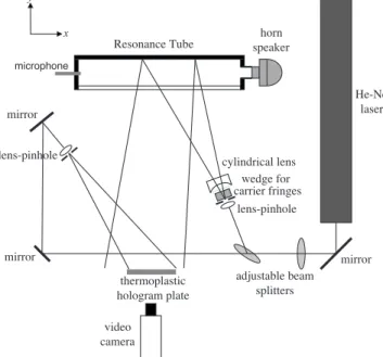
The experiment used a typical holography setup as shown

in Fig. 1. The light source was a 50 mW He–Ne laser

共␭= 633 nm兲. The object and reference beams were

ex-panded with a pinhole lens system. The object beam was further spread in the horizontal direction by a plano-concave cylindrical lens to better illuminate the resonance tube. A transmission hologram was recorded with a Newport thermo-plastic holographic camera, which records and develops the

holographic image on a thermoplastic plate in situ. A video camera was used to look through the thermoplastic plate to-ward the object to record holographic images and fringe pat-terns on video tape for later analysis.

In the experiments described in Refs.14and15the object beam was projected directly through the resonance tube be-fore falling on the holographic plate. We used a resonance tube with only one transparent face and reflected the object beam off the back wall of the resonance tube, which had been painted with flat white paint. Reflecting the object beam off the back wall of the resonance tube had the advantageous effect of allowing the observation of fringes in a time-average hologram for sound pressure levels below 150 dB instead of 165 dB as reported in Refs.14 and15. This dif-ference is significant because once the sound pressure level exceeds 150 dB, sinusoidal sound waves begin to change their shape due to nonlinear effects and the speed of sound begins to depend on the pressure amplitude. Keeping the sound pressure levels low enabled us to predict the fringe patterns without having to include nonlinear effects in the theory.

Figure 2 shows a close-up photo of the resonance tube

used in this experiment. The tube interior has a length of Lx= 61.0 cm, a rectangular cross-section of Ly= 6.4 cm and

Lz= 7.0 cm. The top, bottom, and back walls were made

from 0.25 in. steel, both ends were 0.5 in. steel, and the transparent front face was 0.5 in. plexiglass. A ruled grating was attached to the outside of the tube so fringe widths and wavelengths could be measured. The horn driver was con-nected to the resonance tube with a fitted coupling that screwed into the 0.5 in. steel plate end wall. The sound pres-sure levels inside the tube were meapres-sured by inserting a 0.25 in. diameter B&K type 4156 high-intensity microphone through a hole drilled into the end of the tube opposite the driver. The output of the microphone was observed in the frequency domain using a Stanford Research Systems SR785 FFT analyzer. The microphone-analyzer system was cali-brated to a 124 dB signal at 250 Hz using a B&K 5152 pistonphone. The resonance frequencies of the resonance tube were determined using the swept-sine analysis feature of the frequency analyzer with a frequency resolution of

⫾2 Hz.

as a function of mode numbern. The dashed trendline in the plot represents the calculated resonance frequencies of a closed-closed tube of lengthLx= 0.61 m,

fn= nc 2Lx

, 共1兲

withc= 342 m/s, corresponding to the speed of sound in the laboratory environment at a temperature of 18 ° C. The hori-zontal line in Fig.3indicates the cutoff frequency,16,17above which it is no longer guaranteed that only plane waves will

exist. The cutoff frequency depends on the depth Ly and

heightLzof the tube, f_cutoff= c 2␲

冑

冉

冊

冉

冊

whereᐉ andmare integers used to identify modes in which

the cross-sectional distribution of pressure varies due to standing waves between the side walls of the waveguide.

According to Eq. 共2兲 the first nonplane wave mode

共ᐉ= 0 , m= 1兲was expected at 2443 Hz, so we were guaran-teed to observe plane waves only below this frequency. The holographic images discussed later in this paper are for the

n= 6 plane wave mode that was experimentally observed at

1698⫾2 Hz, which is within 1% of the theoretical value.

III. REAL-TIME HOLOGRAPHIC INTERFEROGRAMS

Real-time holographic interferometry is useful for real-time observation of slow changes in the refractive index of a material8and small static deflections of an object.18For this experiment it provided a means of visualizing the standing sound wave inside the resonance tube. First, a phase holo-gram of the resonance tube was recorded onto the thermo-plastic plate with the sound turned off. The holographic im-age was then viewed with the object beam still on so that the virtual object viewed through the hologram was superim-posed on the actual object. Carrier fringes were added to the holographic image by displacing the object beam via rotation of a glass wedge inserted in front of the object beam pinhole,

as shown in Fig.1. When viewing a real-time hologram, any

slight deflection of the object causes the carrier fringes to move, and a steady state vibration causes the carrier fringes to blur. In our case the carrier fringes blurred because the effective object path length varied due to changes in the re-fractive index as the pressure amplitude of the standing wave oscillated sinusoidally inside the resonator tube. Petersen et al.15used an acoustic-optic modulator to strobe their laser so that the object was illuminated once per cycle of the standing wave, effectively freezing the carrier fringes in place. They were able to watch the strobed carrier fringes shift position as the amplitude of the sound wave was increased. In our experiment we utilized the blurring of the carrier fringes to locate the pressure antinodes in the standing wave patterns and measure the wavelengths.

Figure 4 shows a video screen capture of the real-time

holographic image obtained for the standing wave with

fre-quency of 1698 Hz, corresponding to the n= 6 mode of the

resonance tube. Figure4共a兲shows the carrier fringes with the sound turned off. In Fig.4共b兲the sound level inside the reso-nance tube was 140 dB and the carrier fringes are blurred at regular intervals. The regions where the carrier fringes re-main visible correspond to pressure nodes where the pressure and refractive index do not change, and the effective path length of the object beam is unaffected by the sound wave. The regions where the carrier fringes are blurred correspond to pressure antinodes where the pressure and refractive index alternate between maximum and minimum values at the resonance frequency. The distance between two blurred re-gions 共two antinodes兲equals half a wavelength.

0 1 2 3 4 5 6 7 8 9 Mode Number n 0 500 1000 1500 2000 2500 3000 Frequency (Hz) Theory Measured cutoff frequency

for plane waves

Fig. 3. Measured resonance frequencies共⫾2 Hz兲versus mode number for the resonance tube.

He-Ne laser

Resonance Tube _speakerhorn

mirror adjustable beam splitters lens-pinhole lens-pinhole mirror mirror thermoplastic hologram plate video camera microphone wedge for carrier fringes cylindrical lens x y

Fig. 1. Diagram of holography system used to observe standing sound waves.

Fig. 2. Photograph of the resonance tube with dimensions ofLx= 61.0 cm, Ly= 6.4 cm, andLz= 7.0 cm.

Figure 5 shows the wavelengths obtained by measuring the distance between antinodes of the real-time holograms as

a function of mode number n. The dashed curve represents

the expected wavelengths according to ␭= 2Lx/n. The error

bars on the measured data points indicate the uncertainty in locating the exact center of the blurred regions in the real-time holograms.

IV. TIME-AVERAGE HOLOGRAPHIC INTERFEROGRAMS

Time-average holograms were made by exposing the ther-moplastic plate for a long time relative to the period of the standing wave. After the plate was developed the holo-graphic image was viewed with the object beam turned off and the fringe pattern was recorded using a video camera. A number of holograms were made for several of the resonance frequencies of the tube and with increasing sound pressure levels at each frequency. Frame grabber software was used to capture single frame images for further analysis.

Figure6illustrates how the time-average holographic

im-ages for the 1698 Hz, n= 6 mode changed with increasing

sound pressure level. The hologram in Fig.6共a兲corresponds

to a sound pressure level of 140 dB and shows two white fringes located at nodes where the pressure and thus the re-fractive index do not change. The dark fringes are located at antinodes where the pressure and refractive index oscillate with maximum amplitude. As the sound level increases, the two bright regions grow narrower, but their locations do not change because they are located at pressure nodes. The ho-logram in Fig.6共b兲corresponds to a sound level of 145 dB. The dark fringe at the antinode has split and a bright fringe now appears at the antinode. The irradiance of this new bright fringe is much lower than the bright stationary regions at the nodes. Increasing the sound level further to 149 dB in Fig.6共c兲causes a new dark fringe to appear. This dark fringe is itself split and replaced with an additional bright fringe as the sound level increases to 151 dB in Fig. 6共d兲. The three-dimensional aspect of the standing wave is evident in Figs.

6共c兲and6共d兲, which show semicircular fringe patterns on the floor of the resonance tube. This pattern is further illustrated in Fig. 7.

V. THEORETICAL FRINGE PATTERNS

Other papers describing undergraduate experiments with holographic interferometry12,13 have used a simple theory to predict the number of fringes as a function of vibrational amplitude for comparison with measured fringe counts. Be-cause the vibrating object in this experiment is a standing wave in air, it was simple to predict the actual profiles of the fringe patterns, not just the number of fringes. A potential Fig. 4. Real-time holograms with carrier fringes of the resonance tube with

共a兲the sound turned off and共b兲with a 1698 Hz共n= 6兲standing wave at 140 dB共bottom兲. 1 2 3 4 5 6 7 8 9 Mode Number n 0 10 20 30 40 50 60 70 W avelength (cm) Theory Measured

Fig. 5. Wavelength as a function of mode number as measured from the distance between blurred carrier fringes on a real-time hologram compared with theory共dashed curve兲for a closed-closed tube.

Fig. 6. Time-average holographic images for the 1698 Hz共n= 6兲standing wave mode corresponding to sound pressure levels of共a兲142,共b兲145,共c兲 149, and 共d兲 151 dB. Nodes and antinodes are indicated by N and A, respectively.

limitation to such a prediction is the fact that the sound pres-sure levels in question are in the range where nonlinear ef-fects might not be ignorable.

The total pressure associated with a finite amplitude

stand-ing sound wave in a resonance tube of lengthLxand closed

at both ends may be expressed as19

p共x,t兲=P0+ 2pmcos

冉

Lx

x

冊

amplitude fluctuation due to the standing sound wave, andx

is the distance from one of the rigid ends of the tube. The alternating regions of higher and lower pressure cause the refractive index of the gas to change accordingly. A time-average hologram measures irradiance, which depends on the square of the amplitude of the light falling on the hologram plate. Because the time average of sin2_{共␻t兲 equals 1/2, the}

time dependence in Eq. 共3兲 does not matter, and we need

only be concerned with the dependence on positionxto

pre-dict the fringe pattern.

The refractive indexn for air may be calculated from the

relation20

共n− 1兲⫻108= 8342.13 +2 406 030

130 −␴2 +

15 997

38.9 −␴2, 共4兲

where ␴= 1/␭vac and ␭vac has units of ␮m. If the air is at

temperature T in °C and pressure P in pascal, the value in

Eq.共4兲should be multiplied by20 P关1 +P共61.3 −T兲⫻10−10兴

96 095.4共1 + 0.003 661T兲 . 共5兲

As an example, for light from a He–Ne laser

共␭vac= 0.633 ␮m兲 in dry standard air at 18 ° C and 共 atmo-spheric兲 pressure of 101.325 kPa, the index of refraction is n= 1.000 273 66.

Because of the standing sound wave in Eq.共3兲, the pres-sure term in Eq.共5兲varies with locationxalong the length of the resonance tube. This variation means that the index of refraction in Eq.共4兲is a function of position n共x兲. It is this positional variation in the index of refraction that is respon-sible for the blurring of carrier fringes on a real-time holo-graphic image as well as the fringe patterns on a time-average holographic image. The fringes observed in a reconstructed time-average holographic image are due to the

time-average of the phase shift␾ in the object beam due to

the refractive index variation in the resonance tube when the hologram is generated. A phase shift of 2␲corresponds to a

change in object beam path length of one wavelength␭. So

the phase shift of the object beam is predicted by

␾ 2␲=

2Ly⌬n

␭ , 共6兲

where⌬n represents the change in the refractive index of air due to the standing wave andLyis the resonance tube depth.

The factor 2Lyindicates that the object beam passes through

the sound field twice, reflecting off the back wall of the resonance tube. It has been assumed that the object beam light incident on the resonance tube and object beam light reflected back toward the hologram are approximately per-pendicular to the front face of the tube. To account for the spatial dependence of the refractive index, we write the phase difference as

␾共x兲= 4␲Ly⌬n共x兲

␭ . 共7兲

During the recording of a time-average hologram the phase information is recorded as the average of␾共x兲. IfI0共x兲 is the reconstructed holographic image irradiance produced by a hologram with no standing wave present in the reso-nance tube, then the holographic image irradiance with a standing wave present is18

I共x兲=I0共x兲J₀2共兩␾共x兲兩兲, 共8兲 where 兩␾共x兲兩 indicates taking the magnitude of the phase shift due to the refractive index difference andJ0is the zero

order Bessel function.

The peak pressure amplitude in the tube was calculated from the measured sound pressure level Lp in decibels,

pm=

冑

wherep_ref= 20⫻10−6 _{Pa and the}

冑

from rms to peak amplitude. Theoretical predictions of the fringe pattern irradiance for time-average holograms were calculated using Eqs.共3兲–共5兲and共7兲–共9兲.

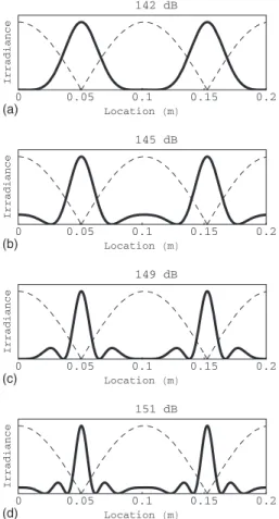
Figure 8 shows the predicted fringe patterns as functions

of position for the same sound pressure levels as the mea-sured fringe patterns shown in Fig.6. The horizontal axis in

Fig.8covers the same distance shown in the photographs in

Fig.6. The dashed curve in each plot in Fig.8represents the

magnitude of the pressure standing wave共zero at nodes and

maximum at antinodes兲. The solid curves represent the fringe pattern irradiance, or the brightness of the hologram image, as predicted by Eq.共8兲. For a sound pressure level of 142 dB, Fig.8共a兲predicts bright fringes at pressure nodes with a dark fringe between at the pressure antinode. When the sound level increases to 145 dB in Fig. 8共b兲, a faint bright fringe appears at the pressure antinode. In Fig. 8共c兲, as the sound level increases to 149 dB, the faint bright fringe at the anti-node has split into two faint bright fringes with a dark fringe between at the antinode. Finally, at 151 dB the bright fringes at the pressure nodes have become thinner, and another faint bright fringe appears at the pressure antinode. The agreement between the predicted fringe patterns in Fig.8and measured

fringe patterns in Fig. 6 with respect to fringe location,

width, and brightness is very good. VI. CONCLUSION

We have described an experiment that uses real-time and time-average holographic interferograms as a tool for study-ing standstudy-ing sound waves. Real-time holography was used to observe the standing waves and to obtain measurements of

back wall of tube corner between back wall and floor

floor of tube

semi-circular fringes on floor

Fig. 7. The three-dimensional nature of the time-average holograms in Fig. 6is evidenced by the semicircular fringes on the floor of the resonance tube.

resonance frequencies and wavelengths. Time-average holo-grams showed the effect of increasing the pressure amplitude on the index of refraction as evidenced by the changes in the fringe patterns. A simple prediction of the fringe pattern matched the measured patterns. The success of this simple theory is largely due to the fact that our experimental setup resulted in the appearance of fringes at sound pressure levels, which are just barely low enough that nonlinear effects may be ignored. A possible extension of this work would be to develop the theory more fully for finite amplitude sound waves including second order nonlinear effects.

ACKNOWLEDGMENTS

The authors would like to thank Newport Corporation and the General Motors Corporation for donating some of the

optical equipment used in this experiment. We would also like to thank the reviewer for providing helpful comments.

a兲_{Electronic mail: drussell@kettering.edu}

b兲_{This experiment began while Hughes was a senior undergraduate student.} He is currently employed by Mantech共www.mantech.com兲.

1_{R. L. Powell and K. A. Stetson, “Interferometric vibration analysis of} three-dimensional objects by wavefront reconstruction,” J. Opt. Soc. Am.

55, 612共1965兲.

2_{R. L. Powell and K. A. Stetson, “Interferometric vibration analysis by} wavefront reconstruction,” J. Opt. Soc. Am. 55, 1593–1598共1965兲. 3_{K. A. Stetson and R. L. Powell, “Interferometric hologram evaluation and}

real-time vibration analysis of diffuse objects,” J. Opt. Soc. Am. 55, 1694–1695共1965兲.

4_{W. Reinicke and L. Cremer, “Application of holographic interferometry} to vibrations of the bodies of string instruments,” J. Acoust. Soc. Am.

48共4兲, 988–992共1970兲.

5_{T. D. Rossing and D. S. Hamilton, “Modal analysis of musical} instru-ments with holographic interferometry,”Applications of Optical Engi-neering: Proceedings of OE/Midwest ’90,关SPIE1396, 108–121共1990兲兴 共SPIE, Bellingham, WA, 1990兲.

6_{T. D. Rossing and H. J. Sathoff, “Modes of vibration and sound radiation} from tuned handbells,” J. Acoust. Soc. Am. 68共6兲, 1600–1607共1980兲. 7_{L. O. Heflinger, R. F. Wuerker, and R. Brooks, “Holographic}

interferom-etry,” J. Appl. Phys. 37, 642–649共1966兲.

8_{H. Fenichel, H. Frankena, and F. Groen, “Experiments on diffusion in} liquids using holographic interferometry,” Am. J. Phys. 52, 735–738

共1984兲.

9_{K.-E. Peiponen, R. Hämäläinen, and T. Asakura, “Laboratory studies of} air flow visualization using holographic interferometry,” Am. J. Phys.

59共6兲, 541–544共1991兲.

10_{K. Lubell and R. Prigo, “Production of real-time holographic} interfero-grams,” Am. J. Phys. 55共9兲, 823–825共1987兲.

11_{A. B. Western and R. Bahaguna, “Simplified production of real-time} holographic interferograms,” Am. J. Phys. 57共6兲, 560–561共1989兲. 12_{R. D. Bahuguna, A. B. Western, and S. Lee, “Experiment in time-average}

holographic interferometry for the undergraduate laboratory,” Am. J. Phys. 56共8兲, 718–721共1988兲.

13_{K. Menou, B. Aduit, X. Boutillon, and H. Vach, “Holographic study of a} vibrating bell: An undergraduate laboratory experiment,” Am. J. Phys.

66共5兲, 380–385共1998兲.

14_{R. F. Salant, W. G. Alwang, L. A. Cavanaugh, and E. Sammartino,} “Vi-sualization of standing acoustic waves using time-average optical holo-graphic interferometry,” J. Acoust. Soc. Am. 44共6兲, 1732–1733共1968兲. 15_{R. W. Peterson, S. J. Pankratz, T. A. Perkins, A. Dickson, and C. Hoyt,}

“Holographic real-time imaging of standing waves in gases,” Am. J. Phys. 64共9兲, 1139–1142共1996兲.

16_{D. D. Reynolds,Engineering Principles of Acoustics, Noise and} Vibra-tion Control共Allyn & Bacon, Boston, MA, 1981兲, pp. 354–359. 17_{K. Meykens, B. V. Rompaey, and H. Janssen, “Dispersion in acoustic}

waveguides—A teaching laboratory experiment,” Am. J. Phys. 67, 400– 406共1999兲.

18_{J. T. Luxon and D. E. Parker,Industrial Lasers and Their Applications,} 2nd ed.共Prentice-Hall, Englewood Cliffs, NJ, 1992兲, pp. 224–230. 19_{D. E. Hall,Basic Acoustics共Krieger, Malabar, FL, 1993兲, pp. 135, 143.} 20_{CRC Handbook of Chemistry and Physics, 95th ed.共McGraw-Hill, New}

York, 1994兲, p. 266. 0 0.05 0.1 0.15 0.2 Location m Irrad i ance 142 dB (a) 0 0.05 0.1 0.15 0.2 Location m Irrad i ance 145 dB (b) 0 0.05 0.1 0.15 0.2 Location m Irrad i ance 149 dB (c) 0 0.05 0.1 0.15 0.2 Location m Irrad i ance 151 dB (d)

Fig. 8. Theoretical predictions of the fringe pattern irradiance corresponding to the measured fringe patterns shown in Fig.6. The dashed curve indicates the pressure amplitude of the standing sound wave. The solid curve repre-sents the brightness of the hologram image. The locations represent the distance from a pressure antinode.