Segmented Mixture-of-Gaussian Classification
for Hyperspectral Image Analysis
Saurabh Prasad,
Member, IEEE,Minshan Cui, Wei Li, and James E. Fowler,
Senior Member, IEEEAbstract—The same high dimensionality of hyperspectral imagery that facilitates detection of subtle differences in spectral response due to differing chemical composition also hinders the deployment of traditional statistical pattern-classification procedures, particularly when relatively few training samples are available. Traditional approaches to addressing this issue, which typically employ dimensionality reduction based on either projection or feature selection, are at best suboptimal for hyperspectral classification tasks. A divide-and-conquer algorithm is proposed to exploit the high correlation between successive spectral bands and the resulting block-diagonal correlation structure to partition the hyperspectral space into approximately independent subspaces. Subsequently, dimensionality reduction based on a graph-theoretic locality-preserving discriminant analysis is combined with classification driven by Gaussian mixture models independently in each subspace. The locality-preserving discriminant analysis preserves the potentially multimodal statistical structure of the data, which the Gaussian mixture model classifier learns in the reduced-dimensional subspace. Experimental results demonstrate that the proposed system significantly outperforms traditional classification approaches, even when few training samples are employed.
Index Terms—Hyperspectral data, information fusion
I. Introduction
T
HE evolution of optical remote sensing over the past few decades has enabled the availability of rich spatial, spectral, and temporal information to remote-sensing analysis. Although this has opened the doors to immense possibil-ities for the analysis of optical remotely sensed imagery, it has also necessitated advancements in signal processing and exploitation algorithms to keep up with advances in the quality and quantity of available data. As an example, the transition from multispectral to hyperspectral imagery (HSI) requires conventional statistical pattern-classification algorithms to be modified to effectively extract useful in-formation from the high-dimensional hyperspectral feature space. By providing a dense sampling of the electromagnetic spectrum in the visible and infrared regions, HSI is expected to provide a highly detailed spectral response per pixel;Manuscript received May 16, 2012; revised September 30, 2012 and January 30, 2013; accepted February 25, 2013. Date of publication April 12, 2013; date of current version November 8, 2013. This material is based on work supported in part by the National Geospatial Intelligence Agency under Grant HM1582-10-1-0001, the National Aeronautics and Space Administra-tion under Grant NNX12AL49G, and the University of Houston, College of Engineering Startup Funds.
S. Prasad and M. Cui are with the Department of Electrical and Computer Engineering and the Geosystems Engineering Research Center at the Univer-sity of Houston, Houston, TX 77004 USA (e-mail: [email protected]; [email protected]).
W. Li and J. E. Fowler are with Mississippi State University, MS 39762 USA (e-mail: [email protected]; [email protected]).
Color versions of one or more of the figures in this paper are available online at http://ieeexplore.ieee.org.
Digital Object Identifier 10.1109/LGRS.2013.2250902
yet, conventional classification algorithms developed and per-fected for multispectral data would often be suboptimal for HSI.
The current state-of-the-art HSI analysis invariably employs some form of dimensionality reduction prior to classifica-tion. Popular approaches include feature/band selection us-ing simple (e.g., stepwise forward selection and backward rejection) or advanced (e.g., genetic algorithms) search algo-rithms, projection-based approaches, such as principal com-ponent analysis (PCA), linear discriminant analysis (LDA), or variants of these methods. Popular supervised classifiers include the quadratic Gaussian maximum-likelihood (ML) classifier and the support-vector-machine (SVM) classifier. In [1], we studied a new approach for HSI classification based on a locality-preserving dimensionality-reduction step—local Fisher’s discriminant analysis (LFDA)—as well as a Gaussian-mixture-model (GMM) classifier. It was shown that LFDA-based dimensionality reduction was effective at preserving the manifold (as well as multimodal statistical distributions) in the dimensionality-reduction projection, and a GMM classifier in this reduced-dimension subspace was hence accurately able to learn class-conditional statistics. We demonstrated that LFDA-GMM is a powerful strategy for hyperspectral classification, outperforming popular algorithms, such as a recursive feature-elimination strategy followed by an SVM classifier [2]. Although LFDA provided effective dimension-ality reduction for GMM classification, it still does not exploit the statistical structure of hyperspectral data to the fullest. In particular, owing to the dense spectral sampling of HSI, successive bands are expected to be highly correlated, and the resulting correlation/mutual-information matrix is expected to be strongly block-diagonal. In this letter, we exploit this structure to partition the hyperspectral feature space into approximately independent subspaces, employing the LFDA-GMM classifier in each subspace. Local classification de-cisions from across all subspaces are then merged using an appropriate decision-fusion strategy. Further, to capture any remnant information in the off-diagonal of the mutual information matrix, we add additional classifiers in the bank that extract and exploit this information. Experimental re-sults demonstrate the efficacy of this segmented classifica-tion strategy—particularly as it relates to robust classificaclassifica-tion using very few training samples (i.e., the small-sample-size scenario).
The remainder of this letter is as follows. In Section II, we review LFDA-GMM and describe the proposed segmented classification strategy. In Section III, we present the pro-posed segmented classifier system, followed by experimen-tal results quantifying and comparing the efficacy of the proposed approach with current state-of-the-art techniques in Section IV. Finally, we provide concluding remarks in Section V.
II. Traditional Single-Classifier Systems
A. Dimensionality Reduction
Dimensionality reduction is a critical preprocessing step for HSI analysis. Owing to the dense spectral sampling of HSI data, the associated spectral information in the hyperspectral bands is typically highly correlated and of high dimension. Hence, dimensionality reduction is commonly applied as a pre-processing step to reduce the dimensionality of the data to en-sure a well-conditioned representation of the class-conditional statistics. Common projection based dimensionality-reduction methods include PCA, LDA, and their many variants. How-ever, these methods are suboptimal at best for hyperspectral images. For example, PCA can potentially discard useful information pertinent to the classification task at hand if such information is aligned along directions of low energy; LDA implicitly assumes that class-conditional probability distribu-tions are homoscedastic Gaussian, etc. A detailed analysis of PCA, LDA, and their variants, and their impacts on classifi-cation performance can be found in the literature [3], [4].
LFDA [5] has been recently proposed as an extension to LDA that, by not restricting the class distributions to be uni-modal Gaussian, is expected to outperform LDA significantly for many practical classification situations. LFDA combines LDA and locality-preserving projection (LPP) [6]—unlike LDA or PCA, LPP is a linear manifold learning technique that seeks a linear map preserving the local structure of neighboring samples in the input space. In other words, after an LPP mapping, neighborhood points in the original input space remain neighbors in the LPP-embedded space, and vice-versa. By invoking a strategy similar to that in LPP, LFDA obtains good between-class separation in the projection while preserving the within-class local structure at the same time. It is hence expected that LFDA will surpass LDA and LPP as a dimensionality-reduction projection when the data is sig-nificantly non-Gaussian, or even severely multimodal. LFDA invokes an affinity matrix that describes the inter-sample relationships and describes the neighborhood relationships of the data in the feature space.
Motivated by traditional LDA, LFDA seeks to find a pro-jection W that optimizes a modified form of Fisher’s ratio: Jlocal(W) =
|WTSlbW|
|WTS lwW|
. Here, SlwandSlbare the local within
and between class scatter matrices, respectively, similar to traditional within and between class scatter matrices [3] with an important exception—they are scaled appropriately by an affinity matrix [1] and [5] in a manner that imparts the useful locality-preserving property to the projection. This weight as-signment provides an important benefit to the traditional LDA formulation—if a class-conditional probability distribution is multimodal, different modes will contribute to the scatter independently, thereby, resulting in a more accurate repre-sentation of multimodal data. This important neighborhood-preserving property ensures that neighbors stay neighbors, and neighbors (e.g., points in different modes) stay non-neighbors under the projection. This approach, hence, results in the scatter matrix estimates that are accurate even when the data violates the homoscedastic Gaussian assumption. The reader is referred to [1] and [5] for more details on LFDA. B. Gaussian Mixture Models (GMMs)
A GMM [7-9] can be viewed as a combination of two or more normal Gaussian distributions. In a typical GMM representation, the probability density function of the data
samples X = {xi}ni=1 in Rd is expressed as the sum of K Gaussian components or modes,p(x) =Kk=1αkN(x, μk, k),
where N(x, μk, k) represents the kth Gaussian component
of the mixture; K is the number of mixture components; and αk, μk, and k are the mixing weight, mean, and
co-variance matrix of the kth component, respectively. These latter three quantities are expressed by the parameter vector ={αk, μk, k}. Once the optimal number of componentsK
per GMM have been determined, the parameters for the mix-ture model can be estimated by the expectation-maximization (EM) algorithm [10], [11]—an iterative optimization strategy. Here, we employ the Bayes information criterion (BIC), [12] which is commonly used for estimating an optimal value ofK in GMMs; BIC() = −2L(,X) +Klog(n), whereL(,X) is the training-data log-likelihood for the GMM model and n is the total number of training samples. The preferred model is the one with the minimum BIC() value—hence, the smallest value of K that minimizes this metric is chosen. In [1], we demonstrated that although the accuracies when using GMMs with both AIC and BIC are similar (and better than other methods), AIC overestimates the number of Gaussians, and hence leads to a higher dimensional feature space. BIC on the other hand provides similar classification performance while providing a lower number of needed mixtures. AIC and BIC are also commonly used when employing GMMs for a variety of other classification tasks [13]–[15].
III. Segmented Mixture-of-Gaussian Analysis
Although the LFDA-GMM combination was effective in [1] for capturing and parameterizing higher-order class-conditional statistical information for classification tasks, it still suffers from one limitation, particularly, insofar as hy-perspectral classification is concerned—the projection from 200 or more spectral bands down to a subspace of dimen-sion an order of magnitude smaller1 can still potentially discard useful information. Further, it has been observed that the correlation/mutual-information structure of HSI is often strongly block-diagonal (e.g., due to the dense spectral sampling) [16]–[18]. It is, hence, possible to segment the hyperspectral space into disjoint subspaces, upon which a single LFDA-GMM classifier is applied. In [16], Prasadet al. proposed a multiclassifier and decision fusion (MCDF) algo-rithm, where such a block-diagonal structure was exploited to partition the spectral space into several contiguous subspaces, following which traditional feature extraction (e.g., LDA) and classification was performed in each subspace. Decision fusion was then invoked to estimate a single class membership func-tion per pixel for classificafunc-tion. In this letter, we extend and en-hance this MCDF algorithm by adding functionality to exploit locality preserving projections and GMM classifiers at the sub-space level and, in doing so, propose and study four key addi-tions: 1) an implementation and optimization of LFDA-GMM in the ensemble-classifier framework; 2) a spectral partitioning metric suitable for LFDA-GMM; 3) a strategy to exploit any residual correlation between subspaces; and 4) an adaptive weight assignment strategy for improved decision fusion.
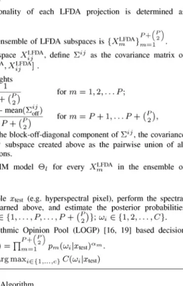
Fig. 1 describes the proposed segmented mixture-of-Gaussian (SMoG) algorithm. First, a bottom-up band-grouping technique is invoked to partition the spectral space into several contiguous subspaces using an approach developed in [16]. To
1In [1], the optimal LFDA dimensionality for single-classifier systems was
found to be in the range 10–20 for a variety of hyperspectral classification tasks.
Fig. 1. The SMoG Algorithm.
optimize for an LFDA-GMM backend, the metric we propose, in this letter, for this spectral partitioning is the product of the local Fisher’s ratio and the average mutual information between all features in each subspace. Although for some hyperspectral imagery datasets, the correlation and mutual information matrices are strongly block-diagonal (facilitating such a spectral partitioning), we have observed for certain datasets, there is a small amount of off-diagonal information. In the traditional spectral partitioning approach, this is dis-carded. To account for any cross-subspace information, we add additional subspaces to our ensemble that are formed by the union of all pairwise subspaces identified by the spectral partitioning above. An LFDA projection is then applied on all subspaces in the ensemble, efficiently capturing the most pertinent discrimination information. Unlike traditional LDA, the dimensionality of an LFDA-projected subspace is typically not bound byC−1, but rather rank(Sm
lb), which may be greater
thanC−1 [1]. To account for any potential correlation (and hence loss of performance) between the subspaces formed by the pairwise union of the original subspaces forming the spec-tral partition, we assign weights to all subspaces{XLFDAm }P+(
P
2)
m=P+1 such that any subspaces that are highly correlated with the existing ensemble {XLFDA
m }Pm=1 are assigned a lower weight, resulting in reducing their power to influence the decision
fusion process and vice-versa. This additional step promotes diversity in the ensemble of classifiers. Following this, a GMM classifier is employed in each subspace. A weighted logarithmic opinion pool (LOGP) decision fusion process [16] is then employed to merge the posterior probabilities from this ensemble into a single class membership function per test sample. Among three popular decision fusion approaches (ma-jority voting, linear and logarithmic opinion pools), we have found that LOGP outperformed all other approaches when the base-classifier in the ensemble is a GMM. This is expected, since LOGP typically results in a unimodal distribution and is less dispersive compared to alternatives [20].
IV. Experimental Results
The efficacy of the proposed SMoG algorithm is studied with three experimental hyperspectral datasets. The first experimental HSI dataset employed was acquired using NASA’s AVIRIS sensor and was collected over northwest Indiana’s Indian Pine test site in June 1992.2 The image represents a vegetation-classification scenario with 145×145 pixels and 220 bands in the 0.4- to 2.45-μm region of the visible and infrared spectrum with a spatial resolution of 20 m. The main crops of soybean and corn in the image are in their early growth stage. The no till,min till, andclean tillindicate the amount of previous crop residue remaining. Approximately 8600 labeled pixels are employed to train and validate/quantify the efficacy of the proposed system. This dataset is partitioned into approximately 1496 training pixels and 7102 test pixels. The other two datasets used in this letter were collected by the Reflective Optics System Imaging Spectrometer (ROSIS) sensor [21]. The image, covering the city of Pavia, Italy, was collected under the HySens project managed by DLR (the German Aerospace Agency). The images have 115 spectral bands with a spectral coverage from 0.43 to 0.86 μm, and a spatial resolution of 1.3 m. Two scenes are used in our experiment. The first one of these is the university area that has 103 spectral bands with a spatial coverage of 610×340 pixels. The second one is the Pavia city center that has 102 spectral bands with 1,096×715 pixels formed by combining two separate images representing different areas of the Pavia city. The numbers of training and testing samples used for University of Pavia dataset are 1476 and 7380, respectively. The numbers of training and testing samples used for Pavia Center dataset are 1477 and 8862, respectively.
Performance of SMoG is compared with traditional single and multiclassifier systems commonly employed for hyper-spectral classification. These include:
1) A multiclassifier system with LFDA-based dimension-ality reduction and GMM as the backend bank of classifiers (MCDF-LFDA);
2) Multiclassifier system with LDA as dimensionality re-duction and quadratic Gaussian ML as the back-end bank of classifiers (MCDF) (Unlike SMoG, these two multiclassifier systems do not take into account the influence of the pairwise subspaces);
3) LFDA-based dimensionality reduction followed by a single GMM classifier (LFDA-GMM) [1];
4) An SVM classifier with an optimized RBF kernel [2]; 5) Dimensionality reduction using regularized Fisher’s
lin-ear discriminant analysis, followed by a quadratic Gaus-sian ML classifier (RLDA) [22].
In this experiment, we used the heat kernel for estimating the affinity matrix in LFDA, which we found to work well for
TABLE I
Average Overall Accuracies (%) and Standard Deviation (in Parentheses) Obtained as a Function of Varying Number of Training Samples
Number of Training Samples per Class 22 30 46 54 70 78
Algorithms Indian Pines Data
SMoG ACC(%) 71(2.8) 75(2.8) 79(0.9) 79(1.3) 81(1.2) 82(0.7) MCDF-LFDA ACC(%) 64(2.6) 67(3.7) 69(2.3) 72(1.1) 71(3.0) 73(2.0) MCDF ACC(%) 58(1.8) 63(2.1) 66(1.2) 69(1.4) 70(1.0) 71(0.7) LFDA-GMM ACC(%) 30(4.8) 46(3.1) 62(2.9) 68(2.5) 73(3.3) 76(2.8) SVM ACC(%) 68(1.9) 71(1.5) 76(1.6) 78(1.6) 80(1.2) 81(0.9) RLDA ACC(%) 38(3.9) 46(2.7) 60(1.9) 64(1.7) 68(1.6) 70(1.0)
Algorithms University of Pavia Data
SMoG ACC(%) 84(0.7) 86(0.9) 88(1.2) 87(0.8) 88(0.8) 88(1.1) MCDF-LFDA ACC(%) 81(2.0) 82(2.6) 87(0.9) 86(1.4) 87(0.7) 87(1.3) MCDF ACC(%) 74(1.6) 78(1.3) 81(0.9) 82(0.9) 84(0.7) 85(0.6) LFDA-GMM ACC(%) 66(1.4) 76(1.5) 84(1.1) 85(0.9) 88(0.6) 88(0.7) SVM ACC(%) 80(1.7) 83(1.0) 85(0.9) 86(0.8) 87(0.6) 87(0.5) RLDA ACC(%) 66(1.4) 72(1.5) 77(1.0) 80(0.8) 82(0.7) 83(0.8)
Algorithms Pavia Center Data
SMoG ACC(%) 88(2.1) 91(1.5) 91(1.4) 92(0.8) 93(0.5) 93(0.6) MCDF-LFDA ACC(%) 87(1.9) 89(1.8) 91(1.4) 91(1.5) 92(0.8) 93(0.7) MCDF ACC(%) 82(2.4) 87(1.2) 88(1.5) 88(0.7) 89(0.7) 89(1.0) LFDA-GMM ACC(%) 75(2.8) 83(2.0) 89(1.4) 90(1.2) 92(1.1) 93(1.0) SVM ACC(%) 85(1.5) 87(1.2) 88(1.1) 88(1.0) 89(1.0) 89(0.9) RLDA ACC(%) 75(2.2) 80(1.8) 85(1.3) 86(1.1) 87(1.0) 88(0.9) TABLE II
Average Overall Accuracies (%) and Standard Deviation (in Parentheses) as a Function of Background Pixel Mixing (i.e., Reduced Pixel Purity)
Background Pixel Mixing (%) 0 20 40 60 80
Algorithms Indian Pines Data
SMoG ACC(%) 75(1.7) 73(2.4) 72(2.4) 60(2.2) 43(2.8) MCDF-LFDA ACC(%) 62(2.2) 60(2.9) 60(2.7) 51(2.4) 38(3.2) MCDF ACC(%) 68(1.3) 67(1.3) 64(1.6) 55(2.1) 40(2.6) LFDA-GMM ACC(%) 65(2.5) 65(1.7) 61(2.5) 53(3.0) 39(3.5) SVM ACC(%) 77(1.3) 75(2.0) 67(3.5) 52(3.9) 32(5.2) RLDA ACC(%) 63(1.6) 63(1.6) 58(1.9) 51(1.6) 39(2.7)
Algorithms University of Pavia Data
SMoG ACC(%) 87(0.5) 87(0.7) 85(1.1) 80(1.2) 64(1.8) MCDF-LFDA ACC(%) 79(1.2) 79(0.8) 77(1.6) 71(1.7) 54(2.3) MCDF ACC(%) 82(0.9) 82(1.0) 80(1.0) 74(1.5) 56(1.1) LFDA-GMM ACC(%) 85(0.8) 85(0.8) 83(1.2) 74(1.7) 54(2.3) SVM ACC(%) 85(1.1) 85(1.7) 83(1.3) 76(2.8) 60(2.5) RLDA ACC(%) 78(0.8) 78(1.0) 77(1.1) 69(1.8) 53(2.6)
Algorithms Pavia Center Data
SMoG ACC(%) 92(1.1) 92(0.7) 92(0.8) 88(0.5) 85(1.3)
MCDF-LFDA MCDF-LFDA ACC(%) 88(1.2) 88(1.0) 87(1.2) 86(1.6) 78(2.6)
MCDF ACC(%) 88(0.9) 87(1.2) 87(1.0) 84(1.2) 75(1.5)
LFDA-GMM ACC(%) 89(1.9) 89(1.1) 87(0.8) 83(1.9) 69(4.1)
SVM ACC(%) 88(0.9) 88(1.1) 86(1.2) 83(1.5) 69(3.8)
RLDA ACC(%) 85(1.5) 85(1.7) 85(1.6) 81(1.6) 68(3.1)
hyperspectral datasets. All the free parameters used in these baseline algorithms, such as σ of the radial basis function (RBF) kernel used in SVM and the regularization parameter in RLDA are estimated by maximizing the classification accuracy with training data via a grid search over the free parameter space.
Performance of SMoG and the baseline systems listed above is measured in two experiments representing challenging real-world scenarios. In the first experiment, we study the classifi-cation accuracy as a function of severity of pixel mixing. This experiment captures situations wherein the spatial resolution of the sensor is insufficient to encapsulate objects (classes) entirely within each pixel, and inadvertent pixel mixing occurs. The smaller the object relative to the pixel size, the more mixing would there be with its background. For example, 70% target abundance indicates the 70% of the target class is linearly mixed with 30% of all other classes in the scene at all spectral wavelengths. It is expected that class-conditional distributions under such conditions would be severely non-Gaussian (possibly strongly multimodal), and hence the SMoG classifier would be very effective under such conditions. In the
second experiment, we vary the number of training samples employed for training the system from a very small number to a reasonably high number. This experiment represents an important restriction when building HSI analysis systems— limited ground-reference (in situ) data. It is expected that the proposed divide-and-conquer component, as well as the LFDA-GMM component in SMoG will effectively account for these two important situations that occur often in many applications involving hyperspectral image analysis.
Tables I and II depict the performance as measured by the overall classification accuracy for the proposed SMoG system, as well as that of the baseline systems listed as a function of the severity of pixel mixing as represented by the target class abundance percentage, and the number of training pixels employed for a vegetation dataset (Indian Pines) and an urban classification task (University of Pavia and Pavia Center). For each experiment, the training samples were selected at random from the datasets multiple times, while the test samples were fixed each time to all the samples in the dataset except the samples that were inducted for training. The mean overall classification accuracies and the standard deviations in the
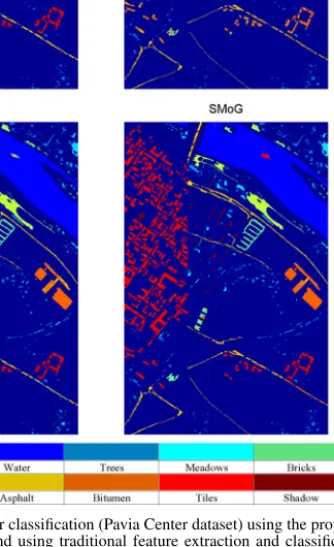
Fig. 2. Ground cover classification (Pavia Center dataset) using the proposed (SMoG) algorithm, and using traditional feature extraction and classification approaches.
accuracy estimates over these multiple runs are reported. It is evident from these results that SMoG outperforms established hyperspectral classification systems. Not only does SMoG need very few training samples (e.g., 20 to 40 samples per class) to learn an appropriate model for each class, it also is su-perior to traditional methods, including SVMs, when the pixel purity in the scene is poor (e.g., when only 40%–60% target is present in the pixels). Fig. 2 shows the ground-truth for the Pavia-Center dataset, and compares ground-cover classifica-tion maps obtained using RLDA, SVM, and SMoG. We would also like to note that we performed additional experiments not reported here due to page limitations, where we compared various spectral partitioning metrics, μ (= JlocalI; Jlocal; and I)—we foundJlocalIworks well for SMoG. By simultaneously exploiting the divide-and-conquer paradigm and the strengths of the LFDA-GMM classifier, one obtains robustness to pixel mixing, and the resulting classification system is effective even when very little training data is employed. To provide an esti-mate of the computational complexity, we compare execution times (training and testing) on an Intel quad-core worksta-tion using Matlab R2012a—SMoG:127s, MCDF-LFDA:114s, MCDF:155s, LFDA-GMM:17s, RLDA:43s, and SVM:298s.
V. Conclusion
In this letter, we proposed a classification algorithm that couples spectral segmentation and mixture-of-Gaussian
classification for hyperspectral image analysis—by exploiting the statistical structure of hyperspectral data to invoke a divide-and-conquer classification paradigm, and by employing LFDA-GMM as the base classifier to accurately model non-Gaussian class-conditional statistics, this system proves to be robust for ground-cover classification. It outperformed traditional feature extraction and classification approaches, as well as the previously developed MCDF algorithm, and resulted in a system that needs few training samples for very effective classification.
References
[1] W. Li, S. Prasad, J. E. Fowler, and L. M. Bruce, “Locality-preserving dimensionality reduction and classification for hyperspectral image analysis,” IEEE Trans. Geosci. .Remote Sens., vol. 50, no. 4, pp. 1185–1198, Apr. 2012.
[2] I. Guyon, J. Weston, S. Barhill, and V. Vapnik, “Gene selection for cancer classification using support vector machines,”Mach. Learn., vol. 46, no. 1-3, pp. 389–422, Jan. 2002.
[3] R. O. Duda, P. E. Hart, and D. G. Stork,Pattern Classification, 2nd ed. New York, NY, USA: Wiley, 2001.
[4] S. Prasad and L. M. Bruce, “Limitations of principal component analysis for hyperspectral target recognition,”IEEE Geosci. Remote Sens.Lett., vol. 5, no. 4, pp. 625–629, Oct. 2008.
[5] M. Sugiyama, “Dimensionaltity reduction of multimodal labeled data by local Fisher discriminant analysis,”J. Mach. Learn. Res., vol. 8, no. 5, pp. 1027–1061, May 2007.
[6] X. He and P. Niyogi, “Locality preserving projections,” in Advances in Neural Information Processing System, S. Thrun, L. Saul, and B. Scholkopf, Eds. Cambridge, MA, USA: MIT Press, 2004.
[7] S. Tadjudin and D. A. Landgrebe, “Robust parameter estimation for mixture model,”IEEE Trans. Geosci. Remote Sens., vol. 38, no. 1, pp. 439–445, Jan. 2000.
[8] M. M. Dundar and D. Landgrebe, “A model-based mixture-supervised classification approach in hyperspectral data analysis,” IEEE Trans. Geosci. Remote Sens., vol. 40, no. 12, pp. 2692–2699, Dec. 2002.
[9] A. Berge and A. H. S. Solberg, “Structured Gaussian components for hyperspectral image classification,”IEEE Trans. Geosci. Remote Sens., vol. 44, no. 11, pp. 3386–3396, Nov. 2006.
[10] N. Vlassis and A. Likas, “A greedy EM algorithm for Gaussian mixture learning,”Neural Process. Lett., vol. 15, no. 1, pp. 77–87, Feb. 2002. [11] A. P. Benavent, F. E. Ruiz, and J. M. S. Martnez, “EBEM: An entropy
based EM algorithm for Gaussian mixture models,” inProc. IEEE Int. Conf. Pattern Recogn., vol. 2. Jun. 2006, pp. 451-455.
[12] G. Schwarz, “Estimating the dimension of a model,”Ann. Stat., vol. 6, no. 2, pp. 461–464, Mar. 1978.
[13] Q. He, J. Yang, Y. Li, J. He, X. Zhang, and W. Li, “Combining GMM, Jensens inequality and BIC for speaker indexing,”Electron. Lett., vol. 46, no. 9, pp. 654–655, 2010.
[14] X. Zhu, C. Barras, S. Meignier, and J. Gauvain, “Combining speaker identification and BIC for speaker diarization,” inProc. Interspeech, vol. 5. Sep. 2005, pp. 2441–2444.
[15] K. Mori and S. Nakagawa, “Speaker change detection and speaker clustering using VQ distortion for broadcast news speech recognition,” inProc. IEEE Conf. Acoust., Speech, Signal Process., vol. 1. 2001, pp. 413–416.
[16] S. Prasad and L. M. Bruce, “Decision fusion with confidence-based weight assignment for hyperspectral target recognition,” IEEE Trans. Geosci. Remote Sens., vol. 46, no. 5, pp. 1448–1456, May 2008.
[17] X. Jia and J. Richards, “Segmented principal components transformation for efficient hyperspectral remote-sensing image display and classifica-tion,”IEEE Trans. Geosci. Remote Sens., vol. 37, no. 1, pp. 538–542, Jan. 1999.
[18] W. Di and M. Crawford, “View generation for multiview maximum dis-agreement based active learning for hyperspectral image classification,”
IEEE Trans. Geosci. Remote Sens., no. 99, pp. 1–13, 2011.
[19] J. A. Benediktsson and J. R. Sveinsson, “Multisource remote sensing data classification based on consensus and pruning,”IEEE Trans. Geosci. Remote Sens., vol. 41, no. 4, pp. 932–936, Apr. 2003.
[20] G. Givens and P. Roback, “Logarithmic pooling of priors linked by a deterministic simulation model,”J. Comput. Graphical Stat., vol. 8, no. 3, pp. 452–478, 1999.
[21] P. Gamba, “A collection of data for urban area characterization,” inProc. Int. Geosci. Remote Sens. Symp., vol. 1. Sep. 2004, pp. 69–72. [22] T. V. Bandos, L. Bruzzone, and G. Camps-Valls, “Classification of
hyperspectral images with regularized linear discriminant analysis,”
IEEE Trans. Geosci. Remote Sens., vol. 47, no. 3, pp. 862–873, Mar. 2009.