Longitudinal performance analysis of machine learning based Android malware detectors

(1)

Longitudinal performance analysis of machine

learning based Android malware detectors

Suleiman Y. Yerima

Cyber Technology Institute, School of Computer Science and Informatics,

De Montfort University, Leicester, United Kingdom

[email protected]

Sarmadullah Khan

Cyber Technology Institute, School of Computer Science and Informatics,

De Montfort University Leicester, United Kingdom [email protected]

Abstract—This paper presents a longitudinal study of the

performance of machine learning classifiers for Android malware detection. The study is undertaken using features extracted from Android applications first seen between 2012 and 2016. The aim is to investigate the extent of performance decay over time for various machine learning classifiers trained with static features extracted from date-labelled benign and malware application sets. Using date-labelled apps allows for true mimicking of zero-day testing, thus providing a more realistic view of performance than the conventional methods of evaluation that do not take date of appearance into account. In this study, all the investigated machine learning classifiers showed progressive diminishing performance when tested on sets of samples from a later time period. Overall, it was found that false positive rate (misclassifying benign samples as malicious) increased more substantially compared to the fall in True Positive rate (correct classification of malicious apps) when older models were tested on newer app samples.

Keywords—Android malware detection, longitudinal performance analysis, static analysis, Machine Learning, Android security

I. INTRODUCTION

Android is the leading mobile operating system worldwide with nearly 75% market share as at January 2019 [1]. Its popularity, coupled with the availability of numerous third-party Android app distribution channels makes it a prime target for malware. It is estimated that more than 25 million mobile malware samples have been seen in the wild as at September 2018 [2], and majority target the Android platform. With the increase in Android malware in recent years, substantial research effort has been directed towards machine learning based detection. Several works have proposed and investigated machine learning based Android malware detection based on dynamic and/or static features.

Most of the existing studies on machine learning based malware detection have presented performance results using conventional methods that do not consider time periods or the age of the testing samples. Despite the proliferation of machine learning based malware detection research, there are hardly any studies that provide a comprehensive longitudinal view of performance. Hence, in this paper, a longitudinal performance analysis of machine learning based Android malware detectors is presented. The aim of the study is to investigate the extent of performance decay over time for various machine learning classifiers trained with features extracted from date-labelled benign and malware samples. The classifiers are then tested on benign and malware samples from a later time period, thus mimicking true zero-day scenario that gives a more realistic view of performance than traditional evaluation approach. The classifiers studied include Naïve Bayes (NB), Support Vector Machines (SVM), Random Forest (RF), J48 Decision Tree and Simple

Logistic (SL). These have been trained using 350 features obtained from static based analysis of each of the apps in the corpora. The apps used in the experiments are date-stamped between February 2012 and January 2016, i.e. the time they first appeared.

The rest of the paper is organized as follows: Section II discusses related work, while Section III presents methodology and the experiments performed. Section IV presents the results and discussion of results and Section V is the conclusion and future work.

II. RELATEDWORK

As mentioned earlier, several works exist that focus on machine learning based detection of Android malware. They can be categorized mainly into static feature-based and dynamic feature-based. A third category combines the two into a hybrid approach.

In [3], an iterative classifier fusion system is developed for the detection of Android malware, based on hybrid static

and dynamic features including permissions, dalvik opcodes,

control-flow graph (CFG) and call graph. Their approach uses a general-purpose meta-procedure to iteratively select features for a given base classifier within the multi-tier iterative classifier fusion system (ICFS). The paper used the well-known MalGenome dataset (consisting of malware samples collected between 2011 and 2012). Although, their results compared ICFS outcome to those from traditional classifiers using stratified 10-fold cross validation, the paper did not present a longitudinal view of the system’s performance.

DroidFusion [4] is a novel classifier fusion approach for Android malware detection which was evaluated on static

features i.e. permissions, API calls, intents, commands, and

other static app properties. The system applies a set of ranking-based algorithms to combine base classifiers in order to improve the overall prediction accuracy. Experiments were performed using samples from MalGenome, Drebin [24], and McAfee datasets to evaluate the system. In the paper, conventional stratified 10-fold cross validation as well training/validation/testing ratio were used to evaluate performance with no longitudinal performance results on time-labelled samples presented.

PIndroid [5] is a permissions and intents based

framework for identifying malware apps. It uses a

combination of permissions and intents coupled with

ensemble learning methods to detect malware. Evaluation is based on conventional 10-fold cross-validation and 80:20 training/testing ratio. The reported accuracy in the paper is 99.8% when tested on 1,745 apps. DroidSieve [6] is an Android malware classifier based on static analysis that is designed to be fast, accurate and resilient to obfuscation. It

(2)

exploits obfuscation-invariant features and artefacts introduced by obfuscation mechanisms used in malware. DroidSieve achieved up to 99.82% accuracy for malware detection and 99.26% accuracy for family identification when tested on over 100K malware and benign apps. W. Wang et al. [7] presented a system for detecting Android malware and categorization of benign apps using ensemble of classifiers. They employed 11 different types of static

features including requested permissions, filtered intents,

suspicious API calls, hardware features, code-related information etc. The ensembled base classifiers include Naïve Bayes, Random Forest, SVM, KNN, and CART. The system was tested on 116,028 app samples achieving 99.39% detection accuracy. Paper [8] also considered an ensemble of various classifiers but experimented on a more limited number of samples to obtain 95.6% accuracy with the best ensemble model.

DroidEnsemble [9] also utilizes static features like

permissions, hardware features, filtered intents, restricted API calls, used permissions, code patterns and function call graphs with an ensemble of SVM, KNN and Random Forest. It was evaluated on 1386 benign apps and 1296 malapps achieving a detection accuracy of up to 98.4%. Some papers such as [10], [11], [12], [29] and [30], employ static analysis-based opcode features with machine learning for Android malware detection. Other papers utilize tools such as Droidbox [13] or Dynalog [14] to extract dynamic features [15] for training machine learning based classifiers. Papers [16]-[21] also present dynamic analysis-based work for Android malware detection, while [22], [23], [31] and [32] use both static and dynamic features.

In all of these existing Android malware detection research papers, long term performance and longitudinal resilience is not investigated. The authors of [27] evaluated their ensemble learning based malware detection system called EnDroid on testing samples that were from a distinct time period from the training samples; however, their work was not an extensive longitudinal evaluation. The work only used 5K benign samples covering a few months (January 2017 to March 2017) and 5K malware samples considered to be post-2015 from AndroZoo for validation (testing). The training samples used consisted of 5213 malware apps from the Drebin dataset (considered to be pre-2015) coupled with 8806 benign apps dated April 2016 to Sept. 2016. Their experiments were intended to validate the performance of EnDroid rather than present a timeline analysis of performance. In [33], a framework called Transcend is proposed for detecting the onset of performance decay i.e. concept drift in machine learning based malware classification models. Transcend is designed to detect aging classification models in vivo during deployment by using a statistical comparison of samples seen during deployment with those used to train the model. It then raises a red flag before the model starts making consistently poor decisions due to out-of-date training. Unlike Transcend, this paper does not aim to provide a detection solution for concept drift but focuses on investigating the extent of drift for Android malware detection models using time-labelled samples from 2012 to 2016.

A possible reason for the scarcity of longitudinal performance studies in the current literature could be lack of access to suitable time-labelled datasets. Nevertheless, due to the evolution of malicious apps, evaluating the

performance over time is important to gain a realistic outlook on the systems being designed for their detection. The study in our paper therefore presents a complementary view to the current results published in the literature, by focusing on the longitudinal performance of the machine learning based Android malware detection.

III. METHODOLOGYANDEXPERIMENTS

A. Datasets

For the purpose of our study, datasets were created from a set of benign and malware apps that were each labelled by

their hash value and date seen. The dates ranged from 14th

February 2012 to 16th January 2016. This initial set of 36,183 applications contained 13,805 malware apps and

22,378 benign (clean) applications from McAfee (Intel

Security) and have been utilized in our previous work [4]. The apps were processed using a bespoke APK analysis tool developed in Python to extract static features. This resulted in a feature dataset that was sorted out according to the dates and then separated into four groups consisting of data for apps from 2012, 2013, 2014 and 2015-2016 respectively. These feature datasets were used to train the machine learning classifiers which were subsequently evaluated in line with the objective of this study. The numbers of the malware and benign apps represented in the feature dataset for each year are shown in Table I. It was decided to merge the 2016 data with the 2015 data because of the relatively small size of the 2016 samples (since only January 2016 apps were present in the collection). Moreover, the apps from the 2015-2016 date range were intended solely to be used for testing during the experiments. For this reason, merging the 2015 and 2016 samples would not defeat the aim of the study.

TABLE I. DATASET STATISTICS. NUMBER OF SAMPLES OF EACH CLASS REPRESENTED IN THE FEATURE DATASET USED FOR THE

EXPERIMENTS. 2012 2013 2014 2015-2016 Malware 512 (24.2%) 1959 (37.4%) 1491 (30.2%) 9843 (41.2%) Benign 1601 (75.8%) 3272 (62.6%) 3448 (69.8%) 14057 (58.8%) Total 2113 5231 4939 23900

B. Application features extraction

The features used to create the training and testing sets were obtained from the apps through the bespoke APK analysis tool mentioned earlier. The tool enables automated feature extraction from Android apps. It is capable of

extracting permissions and intents from the APK manifest

file as well as API calls from the dex file (through automated

reverse engineering). In addition, the tool enables us to check

for the presence of embedded .dex, .jar, .zip, .so and .exe

files (or files of any extension) within the APK. Furthermore, code from system libraries and third-party ad libraries were filtered out during the feature extraction process using a list of commonly used ad libraries from [25]. An overview of the utilised feature extraction process can be found in [4].

(3)

In total, 350 features were extracted from the apps, and

these consisted of API calls, permissions, intents, and other

attributes (e.g. command strings, presence of embedded

executables etc.). All 350 features are present in the feature datasets that were used in the experiments presented in this paper. Table II shows a partial list of the extracted features; the full list is available at [26]. The 350 features provided the input vectors that are used to represent each app in the feature datasets. The datasets are organized into a matrix of input vectors saved in .csv files for training the machine learning classifiers. Each app is represented as a row of feature vectors, with each column of the vector corresponding to a given feature and represented by a ‘1’ if present or a ‘0’ if absent from the app. The last column carries the class label of ‘malware’ or ‘benign’.

TABLE II. A SUBSET OF THE STATIC FEATURES EXTRACTED FROM THE

APPS USING THE PYTHON-BASED AUTOMATED STATIC ANALYSIS TOOL.

FULL LIST OF FEATURES IS AVAILABLE AT [26].

Features Category

Ljava/util/Timer.schedule Utilities API

READ PHONE STATE Permission

getDeviceId (TelephonyManager) Framework res. API Ljava/net/URL.openStream System res. API Ljava/io/FileOutputStream.write System res. API

Class.getClassLoader DVM res. API

Ljava/lang/System.loadLibrary DVM res. API intent.action.SMS RECEIVED Intent

SEND SMS Permission

getConnectionInfo (WifiManager) System res. API getSubscriberId (TelephonyManager) Framework res. API intent.action.PHONE STATE Intent

getWifiState (WifiManager) System res. API

intent.action.SEND Intent

Ljava/io/File.mkdir System res. API .open (AssetManager) Framework res. API

chown Command string

RECEIVE SMS Permission

Ljava/lang/Runtime.exec DVM res. API .read (ZipInputStream) Utilities API

C. Machine learning classifires and evaluation metrics

The machine learning classifiers evaluated in the longitudinal performance study include Naïve Bayes (NB), Simple Logistic (SL), Random Forest (RF), Support Vector Machine (SVM), and J48 Decision Tree. For the evaluation, four metrics are considered: True Positive Rate (TPR), False Positive Rate (FPR), Overall accuracy (ACC) and Weighted F-measure (W-FM) [4]. TPR represents the rate of correct classification of the malicious applications, while FPR represents the rate of misclassification of the clean (benign) applications.

IV. RESULTSANDDISSCUSSIONS

In this section, the results of the experiments undertaken to analyse the longitudinal performance of the machine learning classifiers are presented. The discussion of results

will be split into three subsections. Each subsection will focus on evaluating machine learning models trained using the feature dataset of samples from 2012, 2013, and 2014 respectively.

A. Experiment 1: Analysis of models trained with 2012 samples

In this subsection, the results of experiments on machine learning detectors trained with 2012 data is presented. In order to examine the longitudinal performance, these models are evaluated on the 2013, 2014 and 2015-2016 datasets described in section III-A. The 2012 models were trained with the available 512 malware and 1061 clean samples’ feature datasets (Table I).

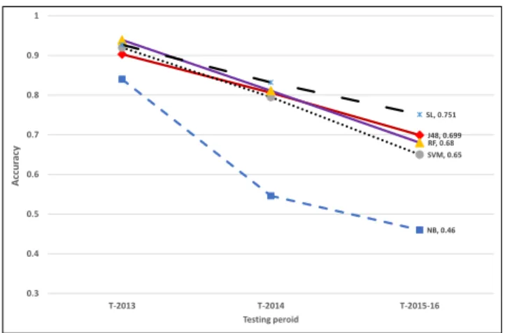
From Fig. 1, it can be noted that the overall classification accuracy decreases for all the classifiers when tested on 2013, 2014, and 2015-16 datasets respectively. Table III shows the numerical results; full results including TPR, FPR and W-FM can be seen in the Appendix (Tables VI and VII). NB classification accuracy decreased from 84% (2013) to 54% (2014) and then down to 46% (2015-16). J48 went from 90.3% on 2013 data, to 80.6% on 2014 data, and down to 69.9% on 2015-2016 data. For SVM (linear) it was 92% (2013), 79.5% (2014) and 65% (2015-16) respectively. RF had 93.9% (2013), 81.1% (2014), and 68% (2015-16). SL started with 92.7% (2013) then dropped to 83.2% (2014) and 75.1% (2015-2016).

If we imagine that this scenario emulates a zero-day situation where emerging apps were tested as they appear, then RF experienced a 28% decline in overall accuracy over the time period 2013 to 2016. SL can be said to have declined by 19% in overall accuracy over the same time period. The lines in Fig. 1 illustrate clearly the drop in the accuracy exhibited by all the 2012 trained models.

NB, 0.46 J48, 0.699 SVM, 0.65 RF, 0.68 SL, 0.751 0.3 0.4 0.5 0.6 0.7 0.8 0.9 1 T-2013 T-2014 T-2015-16 A cc u rac y Testing peroid

Fig. 1: Average accuracy of models trained on the 2012 samples and evaluated on the 2013, 2014 and 2015-2016 samples respectively.

TABLE III. AVERAGE ACCURACY (2012 TRAINING) T-2013 T-2014 T-2015-16 NB 0.840 0.546 0.460 J48 0.903 0.806 0.699 SVM 0.920 0.795 0.650 RF 0.939 0.811 0.680 SL 0.927 0.832 0.751

(4)

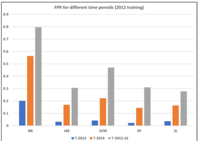
In Fig. 2, the TPR results for all the machine learning classifiers are depicted for the training on 2012 data. Although there are performance drops as the models are tested on 2013, 2014 and 2015-16 data, it is to a lesser degree than the progressive rise in FPR shown in Fig. 3 (numerical results are in the Appendix). This implies that the drop in overall accuracy of the models are impacted more by the misclassification of clean apps than the misclassification of malware apps. 0 0.1 0.2 0.3 0.4 0.5 0.6 0.7 0.8 0.9 1 NB J48 SVM RF SL

TPR for different time peroids (2012 training)

T-2013 T-2014 T-2015-16

Fig. 2: True Positive Rate (malware detection rate) of models trained on the 2012 samples and tested on the 2013, 2014 and 2015-2016 samples respectively. 0 0.1 0.2 0.3 0.4 0.5 0.6 0.7 0.8 0.9 NB J48 SVM RF SL

FPR for different time peroids (2012 training)

T-2013 T-2014 T-2015-16

Fig. 3: False Positive Rate (benign misclassification rate) of models trained on the 2012 samples and tested on the 2013, 2014 and 2015-2016 samples respectively. NB, 0.468 J48, 0.717 SVM, 0.645 RF, 0.681 SL, 0.782 0 0.1 0.2 0.3 0.4 0.5 0.6 0.7 0.8 0.9 1 T-2013-FH T-2013-SH T-2014-FH T-2014-SH T-2015-FH T-2015-SH Accu racy

Testing period (FH- first half, SH- second half)

Fig. 4: Average accuracy of models trained on the 2012 samples and evaluated on six-monthly portions of the 2013, 2014 and 2015-2016 samples respectively.

TABLE IV. DATASET STATISTICS. NUMBER OF SAMPLES OF EACH

CLASS REPRESENTED IN THE FEATURE DATASET USED FOR THE SIX

-MONTHLY EXPERIMENTS.

Malware Benign Total

2013-FH 1078 566 1644 2013-SH 881 2706 3587 2014-FH 613 1628 2241 2014-SH 878 1820 2698 2015-FH 2407 3928 6335 2015-SH (plus Jan 2016) 7436 10129 17565

In Fig. 4, a more granular average accuracy result is presented. This is obtained from splitting the testing samples from each year into two i.e. first half (FH) and second half (SH) to give an approximately six-monthly view of longitudinal performance. The numbers of malware and benign samples in each yearly split are shown in Table IV, and the full results obtained from testing the 2012 models on the six-monthly test sets are shown in Table IX in the appendix. As expected, the performance diminishes more gently on the six-monthly split compared to the previous yearly results. Also, the same trend of more rapid FPR rise compared to TPR decline can be noticed with the six-monthly split results (see Table IX).

B. Experiment 2: Analysis of models trained with 2013 samples

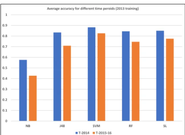
Here, the results of experiments on machine learning detectors trained with 2013 data (1959 malware and 3272 benign) is presented. In order to examine the longitudinal performance, these models are evaluated on the 2014 dataset and 2015-2016 datasets respectively. As was the case with the 2012 models, there is a degradation in overall accuracy during the second testing time period for all classifiers. This can be seen in Table V and Fig. 5. For both time periods, the 2013 SVM model had the highest overall accuracy but also suffered the least loss.

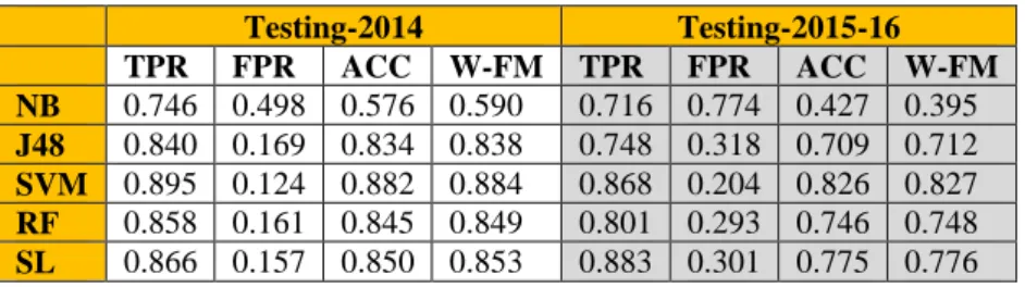
As was the case with the 2012 models, the misclassification of benign applications (see FPR in Fig. 7) contributed more to the overall loss in accuracy compared to the malware misclassification (see TPR in Fig. 6). For example, with the SL model, initial misclassification rate was ~13% for malware and ~16% for benign. In the second time period, misclassification rates for SL were ~12% for malware and ~30% for benign (see Table VIII in the appendix for the numerical results).

TABLE V. AVERAGE ACCURACY (2013 TRAINING) T-2014 T-2015-16 NB 0.576 0.427 J48 0.834 0.709 SVM 0.882 0.826 RF 0.845 0.746 SL 0.850 0.775

(5)

0 0.1 0.2 0.3 0.4 0.5 0.6 0.7 0.8 0.9 1 NB J48 SVM RF SL

Average accuracy for different time peroids (2013 training)

T-2014 T-2015-16

Fig. 5: Average accuracy of models trained on the 2013 samples and tested on the 2014 and 2015-2016 samples respectively.

0 0.1 0.2 0.3 0.4 0.5 0.6 0.7 0.8 0.9 1 NB J48 SVM RF SL

TPR for different time peroids (2013 training)

T-2014 T-2015-16

Fig. 6: True Positive Rate (malware detection rate) of models trained on the 2013 samples and tested on the 2014 and 2015-2016 samples respectively. 0 0.1 0.2 0.3 0.4 0.5 0.6 0.7 0.8 0.9 NB J48 SVM RF SL

FPR for different time peroids (2013 training)

T-2014 T-2015-16

Fig. 7: False Positive Rate (benign misclassification rate) of models trained on the 2013 samples and tested on the 2014 and 2015-2016 samples respectively.

C. Experiment 3: Analysis of models trained with 2014 samples

In this section the results of experiments on machine learning detectors trained with 2014 data (1491 malware and 3448 benign) is presented. In order to examine the longitudinal performance, these models are evaluated on the 2015-2016 dataset only. Table VI shows the results of the 2014-trained models depicting accuracy, TPR, FPR and W-FM. The SL classifier has the highest overall accuracy, slightly better than RF. The RF classifier had the lower FPR compared to SL (see Table VI).

TABLE VI. RESULTS FOR MODELS TRAINED WITH 2014 SAMPLES:

ACCURACY,TPR,FPR AND W-FM Testing 2015-16 ACC TPR FPR W-FM NB 0.758 0.777 0.256 0.759 J48 0.812 0.698 0.108 0.809 SVM 0.872 0.818 0.090 0.872 RF 0.897 0.805 0.039 0.895 SL 0.910 0.871 0.063 0.909

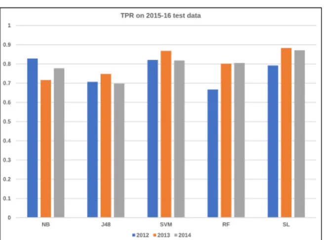
In order to gain a longitudinal performance view, we will compare the results of the 2014 models to the earlier results of testing the 2012 and 2013 models on the 2015-16 data. Comparison graphs are depicted in Figs. 8, 9 and 10.

We can see that the overall accuracy of 2014 models were higher for all the classifiers. Although one can argue that there were more samples in the 2014 dataset than in the 2012 dataset for model training, the 2013 dataset contains more training examples than the 2014 dataset. This implies that the (time) proximity of the 2014 training samples to the (2015-2016) testing set is the more likely contributing factor to better performance. It is worth noting that the 2013 dataset had 468 more malware samples than the 2014 dataset. This may account for better TPR results for SVM trained with the 2013 compared to when trained with 2014 data. Those of SL and J48 were slightly better for 2013 compared to 2014 as well (Fig. 9). Fig. 10 shows that FPR were lowest for 2014 trained models. These results (in Figs. 9 and 10) again highlight that the performance on the benign samples account for more of the loss in overall accuracy (in Fig. 8).

One factor that may contribute to the diminishing performance is the feature set used in training the machine learning algortihms. Over time, some of the features could become less discriminative for the following reasons: (a) more sophisicated evasive techniques appearing more frequently in the malware apps thus making it problematic to extract some features that were previously common. (b) the evolution of the benign apps as more programmers use newer and advanced features, which when used as indicators could trigger more false positives.

0 0.1 0.2 0.3 0.4 0.5 0.6 0.7 0.8 0.9 1 NB J48 SVM RF SL

Overall accuracy on 2015-16 test data

2012 2013 2014

Fig. 8: Overall accuracy of 2012, 2013 and 2014 models when tested on 2015-2016 samples.

(6)

0 0.1 0.2 0.3 0.4 0.5 0.6 0.7 0.8 0.9 1 NB J48 SVM RF SL TPR on 2015-16 test data 2012 2013 2014

Fig. 9: True positive rate of 2012, 2013 and 2014 models when tested on 2015-2016 samples. 0 0.1 0.2 0.3 0.4 0.5 0.6 0.7 0.8 0.9 NB J48 SVM RF SL FPR on 2015-16 data 2012 2013 2014

Fig. 10: False positive rate of 2012, 2013 and 2014 models when tested on 2015-2016 samples.

The top 10 most occuring features in the benign samples within each dataset (by year) are shown in Table X in the Appendix. From the table, it can be observed that different features appear in the top 10 for each year’s set. The 2012

top 10 benign features were dominated by permissions i.e.

INTERNET, WRITE_EXTERNAL_STRORAGE, WAKE LOCK, READ PHONE STATE, ACCESS NETWORK STATE and RECEIVE BOOT COMPLETED. For 2013, the same top 10 is maintained but in a different order. The

2014 dataset however, is dominated by API function calls

with only 3 permissions present. For the 2015-16 set, only 2

permisisons remain in the top 10 for benign class. The variation in the features shown in Table X indicates that the benign apps are being characterized differently over time by the features utilized in this study, which could be due to the changes in the way the newer benign apps were being programed.

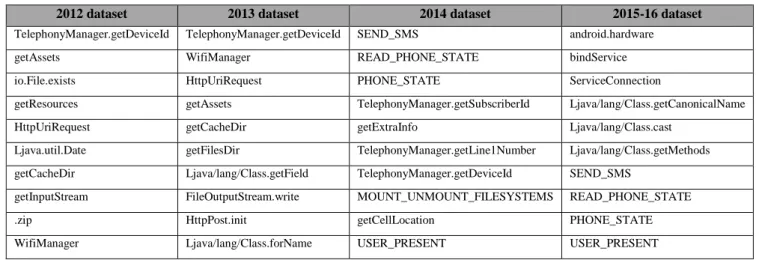
Table XI shows the top 10 features with the highest

information gain for each of the datasets. The information

gain [28] calculates the relevance of a feature or the

information provided by a feature using entropy. The total information gain of the top 10 for each dataset are as follows: 2012 = 2.134; 2013 = 3.379; 2014 = 1.047; 2015-16 = 1.907. This confirms that the predictive power of the features

diminished over time since the total information gain present

in the top features was reduced. Note also that the top features in the newer datasets were different from those in the older ones. Which means that features that were previously discriminative lost some of their predictive power

in the later time peroids. Therefore, it becomes apparent that in addition to peroidic re-training with newer samples, further measures that can be applied to mitigate the loss of the features’ predictive power will ultimately contribute to reducing the diminishing performance over time.

V. CONCLUSION AND FUTURE WORK

As more samples become available, it is expected that the models used in the detection of Android malware will be retrained to improve their performance. However, a longitudinal view of performance can give better insight into the robustness of the models. It can also inform the re-training strategy to be adopted. This particular study shows that based on the static features used for the training, the machine learning models become much less accurate in recognizing benign samples over time. Future work may investigate whether a different set of features such as opcodes could show better longitudinal resilience. Future work would also focus on developing schemes and techniques to mitigate the diminishing performance of the machine learning based malware detectors.

REFERENCES

[1] http://gs.statcounter.com/os-market-share/mobile/worldwide [2] McAfee Labs, “McAfee Labs Threats Report” Sept. 2018, pp. 10–11. [3] J. Abawajy and A. Kelarev, "Iterative Classifier Fusion System for

the Detection of Android Malware," in IEEE Transactions on Big Data, 2017. doi: 10.1109/TBDATA.2017.2676100

[4] S. Y. Yerima, and S. Sezer ‘DroidFusion: A Novel Multilevel Classifier Fusion Approach for Android Malware Detection’ IEEE Transactions on Cybernetics, January 2018, PP. 1-14. Doi:10.1109/TCYB.2017.2777960

[5] F. Idrees, M. Rajarajan, M. Conti, T. M. Chen, Y. Rahulamathavan. PIndroid: A novel Android malware detection system using ensemble learning methods. Computers & Security, Vol 68, July 2017, pp. 36-46.

[6] G. Suarez-Tangill, S. K. Dash, M. Ahmadi, J. Kinder, G. Giacinto, L. Cavallaro, ‘DroidSeive: Fast and accurate extraction of obfuscated Android malware’ CODASPY 2017, Arizona, USA, March 2017. [7] W. Wang, Y. Li, X. Wang, J. Liu, X. Zhang ”Detecting Android

malicious apps and categorizing benign apps with ensemble classifiers” Future Generation Computer Systems, 2017, ISSN 0167-739X.

[8] N. Milosevic, A. Dehghantanha, K.-K. R. Choo ”Machine Learning aided Android malware classification” Computers & Electrical Engineer- ing, Volume 61, July 2017, pp 266-274.

[9] W. Wang, Z. Gao, M. Zhao, Y. Li, J. Liu and X. Zhang, "DroidEnsemble: Detecting Android Malicious Applications With Ensemble of String and Structural Static Features," in IEEE Access, vol. 6, pp. 31798-31807, 2018. doi: 10.1109/ACCESS.2018.2835654 [10] B. Kang, S. Y. Yerima, S. Sezer and K. McLaughlin “N-gram opcode

analysis for Android malware detection” International Journal of Cyber Situational Awareness, Vol. 1, No. 1, Nov. 2016.

[11] R. K. Shahzad, "Android Malware Detection Using Feature Fusion and Artificial Data," 2018 IEEE 16th Intl Conf on Dependable,

Autonomic and Secure Computing,

(DASC/PiCom/DataCom/CyberSciTech), Athens, 2018, pp. 702-709. [12] B. Kang, S. Y. Yerima, K. Mclaughlin, S. Sezer “N-opcode analysis for android malware classification and categorization” 2016 International Conference On Cyber Security And Protection Of Digital Services (CyberSecurity), pp.1–7, doi:10.1109/CyberSecPODS.2016.7502343

[13] DroidBox, Google Archive

https://code.google.com/archive/p/droidbox/

[14] M. K. Alzaylaee, S. Y. Yerima, and S. Sezer, “DynaLog: An automated dynamic analysis framework for characterizing android applications,” 2016 International Conference on Cyber Security and Protection of Digital Services, Cyber Security 2016, 2016.

(7)

[15] M. K. Alzaylaee, S. Y. Yerima, S. Sezer ”Improving Dynamic Analysis of Android Apps Using Hybrid Input Test Generation” In proc. Int. Conf. on CyberSecurity and Protection of Digital Services (Cyber Security 2017), London, UK, June 19-20, 2017.

[16] Dash, S. K., Suarez-Tangil, G., Khan, S., Tam, K., Ahmadi, M., Kinder, J., Cavallaro, L. "DroidScribe: Classifying Android Malware Based on Runtime Behavior," 2016 IEEE Security and Privacy Workshops (SPW), San Jose, CA, 2016, pp. 252-261. doi: 10.1109/SPW.2016.25

[17] Cai, H., Meng, N., Ryder, B., Yao, D.: Droidcat : Unified dynamic detection of android malware (2017)

[18] W.-C. Wu and S.-H. Hung. Droiddolphin: A dynamic android malware detection framework using big data and machine learning. In Proceedings of the 2014 Conference on Research in Adaptive and Convergent Systems, RACS '14, pages 247-252, New York, NY, USA, 2014. ACM.

[19] V. M. Afonso, M. F. de Amorim, A. R. A. Gregio, G. B. Junquera, and ´ P. L. de Geus, “Identifying Android malware using dynamically obtained features ,” Journal of Computer Virology and Hacking Techniques, 2014

[20] A. Mahindru and P. Singh “Dynamic Permissions based Android malware detection using machine learning techniques” 10th Innovations in Software Engineering Conference ISC 2017 Jaipur, India, Feb. 5-7, 2017. pp 202-210.

[21] M. K. Alzaylaee, S. Y. Yerima, and S. Sezer, “Emulator vs real phone: Android malware detection using machine learning,” in Proceedings of the 3rd ACM on International Workshop on Security And Privacy Analytics, ser. IWSPA ’17. Scottsdale, Arizona, USA March 24 - 24, 2017: ACM, 2017, pp. 65–72. [Online]. Available: http://doi.acm.org/10.1145/3041008.3041010

[22] M.-Y. Su, J.-Y. Chang, and K.-T. Fung ”Machine Learning on Merging Static and Dynamic Features to identify malicious mobile apps” In proc. 9th Int. Conf. on Ubiquitous and Future Networks (ICUFN), 2017, Milan, Italy, 4-7 July 2017. pp. 863-867.

[23] Lindorfer, M., Neugschwandtner, M., & Platzer, C. (2015). MARVIN: Efficient and comprehensive mobile app classification through static and dynamic analysis. In Proc. IEEE 39th Annual

Computer Software and Applications Conference (COMPSAC), Volume 2, 422–3433.

[24] D. Arp, M. Spreitzenbarth, H. Malte, H. Gascon, and K. Rieck, “Drebin: Effective and Explainable Detection of Android Malware in Your Pocket,” Symposium on Network and Distributed System Security (NDSS), no. February, pp. 23–26, 2014.

[25] Book, T., Pridgen, A., and Wallach D. S.: Longitudinal Analysis of Android Ad Library Permissions. In Proc. IEEE Mobile Security Technologies, MoST, (2013).

[26] https://sites.google.com/site/suleimanyerima/resources/list-of-features-for-static-analysis

[27] P. Feng, J. Ma, C. Sun, X. Xu and Y. Ma “A Novel Dynamic Android Malware Detection system with Ensemble Learning” IEEE Access, June 2018.

[28] T. M. Cover, J. A. Thomas, Elements of Information Theory, 2nd Edition, John Wiley & Sons, inc., Hoboken, New Jersey, 2006, pp. 41.

[29] T. Chen, Q. Mao, Y. Yang, M. Lv and J. Zhu “TniyDroid: A Lightweight and Efficent Method for Android Malware Detection and Classification” Mobile Informaion Systems, vol. 2018, Article ID 4157156, 9 pages, 2018. https://doi.org/10.1155/2018/4157156. [30] N. Bakhshinejad and Ali Hamzeh “ A New Compression Based

Method for Android Malware Detetction Using Opcodes” 2017 Artificial Intelligence and Signal Processing Conference (AISP), Shiraz, 2017, pp. 256-261. doi: 10.1109/AISP.2017.8324092 [31] L. Xu, D. Zhang, N. Jayasena and J. Cavazos “ HADM: Hybrid

Analysis for Detection of Malware” SAI Intelligent Systems Conference 2016, Septtember 21-22, 2016, London UK.

[32] A. T. Kabakus and I. A. Dogru. “An In-depth Analysis of Android Malware Using Hybrid Techniques” Digital Investigation 24 (2018) pp. 25-33.

[33] R. Jordaney, K. Sharad, S. K. Dash, Z. Wang, D. Papini, I. Nouretdinov & L. Cavallaro “Trancend: Detecting Concept Drift in Malware Classification Models” 26th USENIX Security Symposium, aug. 16-18 2017, Vancouver, BC, Canada.

Appendix

TABLE VII. RESULTS FOR MODELS TRAINED WITH 2012 SAMPLES

Testing-2013 Testing-2014 Testing-2015-16

TPR FPR ACC W-FM TPR FPR ACC W-FM TPR FPR ACC W-FM

NB 0.908 0.201 0.840 0.842 0.799 0.564 0.546 0.555 0.828 0.797 0.460 0.410

J48 0.794 0.032 0.903 0.901 0.749 0.169 0.806 0.810 0.707 0.306 0.699 0.701

SVM 0.859 0.042 0.920 0.920 0.835 0.222 0.795 0.802 0.821 0.470 0.650 0.648

RF 0.874 0.022 0.939 0.939 0.706 0.144 0.811 0.812 0.667 0.310 0.680 0.682

SL 0.866 0.036 0.927 0.927 0.822 0.164 0.832 0.835 0.792 0.278 0.751 0.753

TABLE VIII. RESULTS FOR MODELS TRAINED WITH 2013 SAMPLES

Testing-2014 Testing-2015-16 TPR FPR ACC W-FM TPR FPR ACC W-FM NB 0.746 0.498 0.576 0.590 0.716 0.774 0.427 0.395 J48 0.840 0.169 0.834 0.838 0.748 0.318 0.709 0.712 SVM 0.895 0.124 0.882 0.884 0.868 0.204 0.826 0.827 RF 0.858 0.161 0.845 0.849 0.801 0.293 0.746 0.748 SL 0.866 0.157 0.850 0.853 0.883 0.301 0.775 0.776

(8)

TABLE IX. RESULTS FOR MODELS TRAINED WITH 2012 SAMPLES, TESTED ON 6 MONTHLY PORTIONS OF THE DATASET

TABLE X. TOP TEN MOST OCCURRING FEATURES IN THE BENIGN SAMPLES FOR EACH DATASET (BY YEAR).

2012-benign 2013-benign 2014-benign 2015-16-benign

INTERNET INTERNET INTERNET INTERNET

WRITE_EXTERNAL_STORAGE WRITE_EXTERNAL_STORAGE getResources ACCESS_NETWORK_STATE

WAKE_LOCK ACCESS_NETWORK_STATE ACCESS_NETWORK_STATE getResources

READ_PHONE_STATE getResources IBinder Ljava/lang\Object.getClass

PHONE_STATE IBinder Ljava/lang/Object.getClass IBinder

getResources WAKE_LOCK io.File.exists io.File.exists

ACCESS_NETWORK_STATE RECEIVE_BOOT_COMPLETED Ljava.util.Date io.File.delete

IBinder PHONE_STATE io.File.delete Ljava.util.Date

intent.action.BOOT_COMPLETED READ_PHONE_STATE WRITE_EXTERNAL_STORAGE getInputStream

RECEIVE_BOOT_COMPLETED intent.action.BOOT_COMPLETED getInputStream Ljava/lang/Class.forName

TABLE XI. TOP TEN FEATURES WITH THE HIGHEST INFORMATION GAIN FOR EACH DATASET (BY YEAR).

2012 dataset 2013 dataset 2014 dataset 2015-16 dataset

TelephonyManager.getDeviceId TelephonyManager.getDeviceId SEND_SMS android.hardware

getAssets WifiManager READ_PHONE_STATE bindService

io.File.exists HttpUriRequest PHONE_STATE ServiceConnection

getResources getAssets TelephonyManager.getSubscriberId Ljava/lang/Class.getCanonicalName

HttpUriRequest getCacheDir getExtraInfo Ljava/lang/Class.cast

Ljava.util.Date getFilesDir TelephonyManager.getLine1Number Ljava/lang/Class.getMethods getCacheDir Ljava/lang/Class.getField TelephonyManager.getDeviceId SEND_SMS

getInputStream FileOutputStream.write MOUNT_UNMOUNT_FILESYSTEMS READ_PHONE_STATE

.zip HttpPost.init getCellLocation PHONE_STATE

WifiManager Ljava/lang/Class.forName USER_PRESENT USER_PRESENT

Testing-2013-first-half Testing-2013-second-half Testing-2014-first-half