Tech Report TR-WP Analyzing Virtualized Datacenter Hadoop Deployments Version 1.0

(1)

Longitudinal Analytics of Web Archive data

European Commission Seventh Framework Programme

Call: FP7-ICT-2009-5, Activity: ICT-2009.1.6

Contract No: 258105

Tech Report TR-WP3-6-2.9.2013

Analyzing Virtualized Datacenter

Hadoop Deployments

Version 1.0

Editor: Aviad Pines

Work Package: WP3

Status: Final

Date: 2.9.2013

(2)

Tech Report TR-WP3-6-2.9.2013

Analyzing Virtualized Datacenter Hadoop Deployments

Project Overview

Project Name: LAWA – Longitudinal Analytics of Web Archive data Call Identifier: FP7-ICT-2009-5

Activity Code: ICT-2009.1.6 Contract No: 258105

Partners:

1. Coordinator: Max-Planck-Institut für Informatik (MPG), Germany 2. Hebrew University of Jerusalem (HUJI), Israel

3. European Archive Foundation (EA), Netherlands

4. Hungarian Academy of Sciences (MTA-SZTAKI), Hungary 5. Hanzo Archives Limited (HANZO), United Kingdom

6. University of Patras (UP), Greece

Document Control

Title: Analyzing Virtualized Datacenter Hadoop Deployments Author/Editor: Aviad Pines

Document History

Version Date Author/editor Description/comments

(3)

This paper discusses the performance of Hadoop deployments on virtualized Data Centers such as Amazon EC2 and Elastichosts, both when the Hadoop cluster is located in a single data center, and when it is spread in a cross-datacenter deployment. We analyze the impact of bandwidth between nodes on cluster performance.

Introduction

Map Reduce is a programming model for processing and generating large data sets. It is in common use by the commercial sector, as well as researchers, to process large quantities of data. Among the users of Map Reduce one can find Amazon, Facebook and Yahoo [1] [2].

The typical Hadoop deployment takes place in a server room, or in large deployments, in a data center. In this paper, we aimed to analyze the performance of Hadoop deployments of various sizes in the virtualized data centers provided by two cloud server providers: Amazon [3] and Elastichosts [4].

In addition to investigating Hadoop performance in the cloud, we have deployed Hadoop in between two of Elastichosts’ data centers, and have investigated Hadoop performance across the Internet. The different bandwidth speeds between server, local rack and cluster are a known fact [5], and we have at first expected an order of magnitude drop in bandwidth between a single data-center and an inter-datadata-center Hadoop deployment (both due to the pattern of an order of magnitude drop by distance and by our experience with Internet speeds). We have also expected that Hadoop will have difficulty coping with the larger latency introduced by an Internet link. While we have indeed observed the expected drop in bandwidth, we were surprised to discover that Hadoop does indeed run across the open Internet (at least between data centers).

(5)

The ability to run Hadoop deployments over multiple datacenters has an obvious advantage. Companies can utilize a number of their datacenters in order to run large jobs without being confined to a single location, thus reducing the amount of time it takes to complete a job. In addition data collection can occur in separate locations in the company's geography. Enable computation among the distinct location avoid the need to move the data, costing the company more money for the extra storage.

After analyzing both deployments (Amazon and Elastichosts) we have used the data to create a mathematical model of a Hadoop job execution time. We have used this model to investigate the effects of various variables on the job execution time.

Related Work and Anticipated Impact

Previous work has showed that MapReduce offers a flexible, and effective tool for data processing, proving to be efficient, fault tolerant and highly scalable [6] [2]. It should be noted that since Hadoop's implementation favors homogeneous cluster structure and not deploying it in such a manner so may impede performance work has been carried out regarding the improvement of performance in scenarios where the cluster is heterogeneous [7]. Performance studies of Hadoop have also been conducted, in both regular and virtualized environments [8] [9], but they seem to mostly focus on the total job running times and efficient scheduling of jobs and tasks, and ignore the underlying network performance as uninteresting. A more recent work has been published that studies the effects of network traffic in the confines of a small, 5-node Hadoop cluster [10].

Aside of Hadoop performance, schedulers and protocols for networking traffic within datacenters have also been designed to improve networking performance in data centers and studies have been carried out as to characterize the networking traffic of large data centers [11] [12] [13]. Additionally, work has been done to investigate the advantages of the shift from a monolithic, large, single-site datacenter to smaller, more distributed clouds [14].

It is our aim to expand upon this base of knowledge by contributing input as to the network traffic generated by Hadoop and allow insight into how the network performance potentially affects Hadoop performance. We also aim to show that deploying Hadoop across the Internet is a real possibility.

(6)

Methodology

Hadoop itself provides various metrics about its performance, each task logs its start and end times, the amount of data it has consumed and produced and the amount of time that it ran. This is useful but insufficient since the bandwidth and the idle time statistics of the network is not measured. In order to obtain more detailed metrics we have implemented a Statistic Server which is an additional Hadoop component that serves as a sink for traffic reports. Traffic reports are small descriptors sent from each node in the cluster which detail network transfers by their starting timestamp, duration, size, and type (HDFS Reads, Reducer Inputs or HDFS Writes). By using these traffic reports we were able to measure both the bandwidth at various parts of the job, the typical size of a transfer, and also the total time the network was idle of Hadoop traffic. Care was taken to reduce the volume of this traffic so as to not affect the actual running time of Hadoop jobs on the modified cluster. The statistics server does not provide us the ability to see management traffic, e.g. traffic sent from the Name Node in order to control the execution flow of the job. Since the management traffic is negligible when compared to the rest of the traffic of the Hadoop job, therefore it has no effect on the cluster performance.

Our job of choice was a simple word count benchmark run on the Gutenberg dataset, which is a collection of about 23,000 free books in plain text format (totaling about 10GB of text) and is available from the Gutenberg Project [15]. Our virtualized clusters were of two types: The Amazon EC2 cluster used m1.large instances, which provide 2 computational cores and 7.5GB of RAM. On Elastichosts we’ve specified machines with a single core, 2GB of RAM and a clock setting of 2,000 MHz. In both cases, however, we do not really know which virtualization setup our cluster actually runs on, the load of other VMs on the physical host, or the general networking load in the data center. This is the nature of the cloud environment. For our cluster configuration, we have specified that each machine will have a number of map and reduce slots identical to the number of virtualized cores that it is configured with.

(7)

When calculating our networking metrics we have taken care to omit any transfer which has its source and destination on the same machine. Such transfers are handled by the OS and Hypervisor protocol stacks and do not use any actual networking resources in the data center itself. As such, they do not affect the network load and the link speed does not affect them.

Amazon Deployments

First, we deployed our modified Hadoop onto Amazon EC2. We used EC2 VMs for this, and have not used Elastic Map Reduce as we wanted to manage our machines by ourselves and wanted to use a custom Hadoop version which included our support for statistic gathering. Elastic Map Reduce allows users to execute map-reduce jobs without tinkering with a cluster configuration of the management of individual hosts. The cluster size ranged from 8 to 128 machines with two cores each.

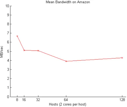
Overall, we wanted to see whether network performance affects the running time of Hadoop jobs and whether running Hadoop over the Internet is possible. At first we wanted to see whether the number of machines involved in the computation would affect the performance of the data center network. The following graph illustrates the effect that the Hadoop cluster size has on the average bandwidth of a network path between two machines in the virtualized datacenter.

(8)

Figure 1: Mean bandwidth per number of hosts on Amazon EC2

(9)

Figure 3: Cumulative transfers for Gutenberg job on Amazon EC2, 64 hosts (128 cores)

It is rather interesting to note that there are very few transfers of map inputs. Indeed, the number of non-local map tasks is extremely small. This is due to the uniform distribution of input blocks on machines (giving each machine the same amount of local input) and the homogeneity of machines across the Hadoop cluster (giving each machine similar processing power to crunch through its local maps). Indeed, the bulk of transfers occur in the shuffle phase, where map outputs get transferred to their reducers.

Elastichosts Deployments

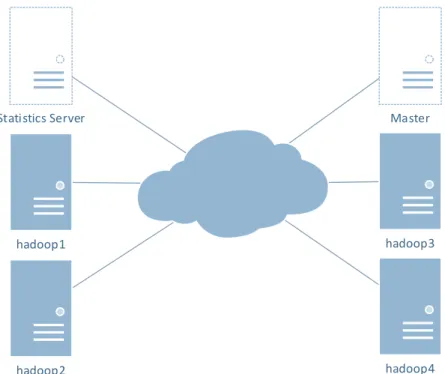
Our second set of experiments centered on benchmarking Hadoop in an inter-datacenter deployment. We have deployed 4 and 16 slave clusters across two Elastichosts datacenters: One was located in San Antonio, Texas, while the other in Los Angeles, California. In both cases, half the machines would be located in each of the data centers. This means that in the 4-machines job, approximately 66% of the traffic was sent through the cross-datacenter link while in the 16-machines job approximately 53% of the traffic was sent through it. In both cases, more than half of the traffic was cross-datacenter.

(10)

Statistics Server hadoop1 hadoop2 Master hadoop4 hadoop3

Figure 4: In the 4-machines deployment, hadoop1 is sending on the intra-datacenter link to hadoop2, and on the inter-datacenter link to hadoop3 and hadoop4, meaning that approximately 66% of its traffic is sent

through the inter-datacenter link.

The RTT for packets between both data centers was about 45ms on average, gathered from 5000 pings that were sent between data centers.

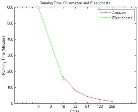
As expected, there is a significant difference between the bandwidth of the two links. An order of magnitude difference was measured between machines not in the same data center and those which are located in the same one. However, the following graph shows us that there is no actual effect on the running time.

(11)

Figure 5: Running time per number of cores on Amazon EC2 and Elastichosts

This is a non-trivial result: The fact that the running time is similar on the 16 core case (with Elastichosts being slightly faster) is not what we expected to see. Network performance between two hosts in the different data centers is comparable to the download speeds of a consumer internet connection, and we expected this to affect computation time, but this was not the case. Upon examining the actual busy-times of the network paths between cluster nodes, we have discovered that network transfers only occurred during, on average, 3% of the computation time on Amazon and 6.3% of the computation time on Elastichosts, with a variance of 0.023 and 0.061 respectively. This leaves the network idle for the vast majority of the job’s runtime and explains this result.

This has led us to try and devise a mathematical model for the computation time of a Hadoop job that would be able to explain this and would enable us to explore the effects of bandwidth on computation time.

A Mathematical Model of Computation Time

Our mathematical model works as follows. We separate the model into two parts, the mapping and shuffle phase and the reduce phase.

(12)

The mapping time can be one of two scenarios – either the map tasks take longer than the shuffle phase or vice versa. Assuming the former, the mapping time will be completing all the map tasks plus the time of a single shuffle for the last map output. On the other hand, assuming that the shuffle phase takes longer than the map phase, then the time will be the first map task time (since the actual copy of data in the shuffle will only start after it), plus the time that it takes to shuffle all the map tasks in parallel to the reducers. We will take the mapping time as the maximum between the two cases.

Let's analyze the first case, where the map tasks take longer than the shuffle. Looking at the mapping phase, and assuming equal distribution of input between all the mappers, the average mapping task will take M_N∙m, where m is the average map execution time, M is the total number of map tasks and N is the number of cores. Now let's look at a single shuffle time. It is the average output of the mapper divided by the number of hosts (all the calculations are done in parallel), and divided by the speed of the network link. Since the cross data center transfer will always be the bottleneck in terms of the network speed, we will use it to see the worst case scenario. Denoting Om as the average output per mapper, lc as the cross data center link speed, we get O_Nm∙_l1_c for a single shuffle time.

Proceeding to the second case, where the shuffle phase takes longer time then the map tasks time, we have the first map tasks plus all the shuffle time, which is a single shuffle time calculated in the previous section, multiplied by the number of map tasks that will have to be shuffled to the reducers. We will get the following for the second case of the map phase:

𝑚

+

𝑂

𝑁 ∙

𝑚

𝑙

1

𝑐

∙

𝑀

𝑁

(1)

And the map phase will be the maximum between the two cases:

𝑚𝑎𝑥

⎩

⎨

⎧

𝑀

𝑁 ∙ 𝑚

+

𝑂

𝑁 ∙

𝑚

𝑙

1

𝑐

𝑚

+

𝑂

𝑁 ∙

𝑚

𝑙

1

𝑐

∙

𝑀

𝑁

(2)

(13)

The reduce phase is the number of reducers we have per host times the average reducer execution time. Denoting R as the total number of reduce tasks and rmax as the maximum reducer execution time, we get the following for the reduce phase:

𝑁 ∙ 𝑟

𝑅

_𝑚𝑎𝑥

(3)

The reason that we are taking the maximum reducer execution time and not the average, is that unlike the mapping phase, where we can assume that Hadoop will uniformly distribute the mapper tasks among the mappers, the reducers accept keys. A single key cannot be distributed among several reducers, making the largest key the bottleneck for the reducer tasks.

This makes our complete model of computation to be

𝑚𝑎𝑥

⎩

⎨

⎧

𝑀

𝑁 ∙ 𝑚

+

𝑂

𝑁 ∙

𝑚

𝑙

1

𝑐

𝑚

+

𝑂

𝑁 ∙

𝑚

𝑙

1

𝑐

∙

𝑀

𝑁

+

𝑟

𝑚𝑎𝑥

(4)

M = Number of map tasks. N = Number of slots.

m = Average map execution time. Om =Average output per mapper. lc = Cross data center link speed.

rmax= Maximum reducer execution time.

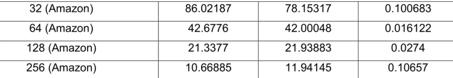
How accurate is our model? We have used the Hadoop metrics to extract the inputs to our

equation from some of the jobs we have executed. The results are illustrated in the following table:

Total Map/Reduce Slots

Estimated Running Time

(minutes)

Actual Running

Time (minutes) Error

4 (Elastichosts) 560.4329 590.3908 0.050742

16 (Elastichosts) 142.9606 151.569 0.056795

(14)

32 (Amazon) 86.02187 78.15317 0.100683

64 (Amazon) 42.6776 42.00048 0.016122

128 (Amazon) 21.3377 21.93883 0.0274

256 (Amazon) 10.66885 11.94145 0.10657

Figure 6: Comparing mathematical model results with actual running times

Where the data collected for each of the variables of the equation were:

Number of Cores Total Number of Map Tasks Average Map Execution Time (Milliseconds) Average Mapper Output (Bytes) Link Speed (K/sec) Total Number of Reduce Tasks Max Reducer Execution Time (Milliseconds) 16 22655 6779 616852.67 6992.15 16 724000 32 22655 6779 616852.67 5353.48 32 362000 64 22655 6779 616852.67 5332.85 64 161000 128 22655 6779 616852.67 4085.54 128 80434 256 22655 6779 616852.67 4085.54 256 40217.0

Figure 7: Data used to estimate the mathematical model results on Amazon EC2

Number of Cores Total Number of Map Tasks Average Map Execution Time (Milliseconds) Average Mapper Output (Bytes) Link Speed (K/sec) Total Number of Reduce Tasks Max Reducer Execution Time (Milliseconds) 4 22655 5919.75 616852.67 810.09 4 97784.5 16 22655 5919.75 616852.67 559.80 16 195569.0

Figure 8: Data used to estimate the mathematical model results on Elastichosts

As we can see, our model, while not being perfect, does follow the general behavior of the Hadoop clusters. This means that we can explore the effects of the input variables on the (estimated) running times.

The most significant difference between the Amazon cluster and the Elastichosts one is that in the latter we have a cross datacenter network link which is significantly slower than the inner

(15)

datacenter bandwidth ranges from 6000 to 7000kb/sec, and the cross datacenter bandwidth is by an order of magnitude slower – it ranges from 560 to 810kb/sec.

Total Map/Reduce slots Amazon Mean Bandwidth Elastichosts in datacenter bandwidth Elastichosts cross datacenter bandwidth 4 6894.53 810.096 16 6992.15 6351.77 559.80 32 5353.48 64 5332.85 128 4085.53 256 4480.24

Figure 9: Comparison of mean bandwidth between Amazon EC2 and Elastichosts

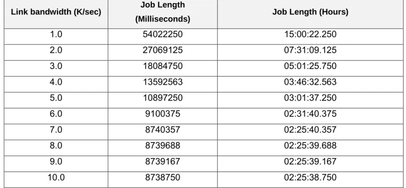
In our formula we choose the slowest link, since it will be the one creating the network bottleneck. We tested different parameters to see how the link bandwidth affects the overall job length.

Link bandwidth (K/sec) Job Length

(Milliseconds) Job Length (Hours)

1.0 54022250 15:00:22.250 2.0 27069125 07:31:09.125 3.0 18084750 05:01:25.750 4.0 13592563 03:46:32.563 5.0 10897250 03:01:37.250 6.0 9100375 02:31:40.375 7.0 8740357 02:25:40.357 8.0 8739688 02:25:39.688 9.0 8739167 02:25:39.167 10.0 8738750 02:25:38.750

Figure 10: Using the mathematical model to compare the effects of the link strength on the job length

We can see that the last significant affect was between the 6k/sec and the 7k/sec, and afterwards the changes are measured only in a few seconds improvement. It seems that network length is not significant at all for the job length, and if you have more than a 7k/sec connection (which is considered slow today even for the average home connection, not mentioning datacenter link

(16)

speeds) upgrading the link bandwidth will not help speeding up the job length. This discovery is not surprising when taking into consideration the time the network was idle, which was as mentioned before 97% of the job lifetime.

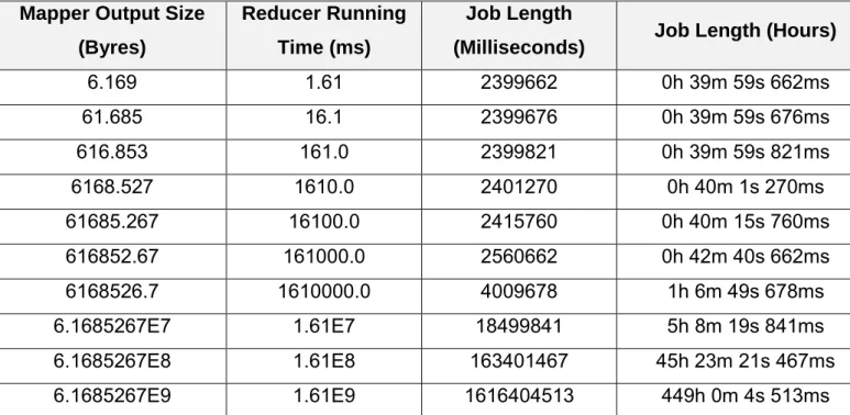
Instead of changing the network link, we can increase the mapper output. This will increase the amount of data we need to transfer and is equivalent do changing the network speed. In our jobs the mapper output was 616852.67 bytes. We increase the mapper output in our model to see how would affect the job length.

Mapper Output Size (Byres) Job Length

6.168526700000001 2560660 0h 42m 40s 660ms 61.68526700000001 2560660 0h 42m 40s 660ms 616.8526700000001 2560660 0h 42m 40s 660ms 6168.5267 2560660 0h 42m 40s 660ms 61685.26700000001 2560660 0h 42m 40s 660ms 616852.67 2560662 0h 42m 40s 662ms 6168526.7 2560678 0h 42m 40s 678ms 6.168526700000001E7 2560841 0h 42m 40s 841ms 6.1685267E8 2562467 0h 42m 42s 467ms 6.1685267E9 6565513 1h 49m 25s 513ms

Figure 11: Using the mathematical model to see the effects of mapper output on job length

We can see that increasing the mapper output size by seven orders of magnitude increases the job length by less than a second, and only when increasing by eight orders of magnitude you can see a difference that can be measured by more than a couple of minutes. This means that even if we have a job that creates vast amount of data, it will not affect the overall job length.

In real jobs however, we expect that increasing the output bytes of the mapper will increase the running time of the reducers, since more input is being sent to them. Under the assumption that the increased output has the same distribution as previously, we can derive the conclusion that each reducer will receive a larger amount of input that is proportional to the increased mapper output. Since the running time is linearly proportional to the input data size [7], we can assume

(17)

that the running time of each reducer will be increased by the same factor of the mapper output increase.

Mapper Output Size (Byres)

Reducer Running Time (ms)

Job Length

6.169 1.61 2399662 0h 39m 59s 662ms 61.685 16.1 2399676 0h 39m 59s 676ms 616.853 161.0 2399821 0h 39m 59s 821ms 6168.527 1610.0 2401270 0h 40m 1s 270ms 61685.267 16100.0 2415760 0h 40m 15s 760ms 616852.67 161000.0 2560662 0h 42m 40s 662ms 6168526.7 1610000.0 4009678 1h 6m 49s 678ms 6.1685267E7 1.61E7 18499841 5h 8m 19s 841ms 6.1685267E8 1.61E8 163401467 45h 23m 21s 467ms 6.1685267E9 1.61E9 1616404513 449h 0m 4s 513ms

Figure 12: Using the mathematical model to see the effects of mapper output and reducer running time on the job length

We can see that the increase in reducer time increase the overall job length, and increasing the data by tenfold only increase the overall running time by less than a factor of two.

Map Phase Tipping Point

Next thing that we wanted to explore is when the tipping point between the mapper time and shuffle time in the map phase occurs. Looking again at the mathematical model, the map phase consists of

(18)

𝑚𝑎𝑥

⎩

⎨

⎧

𝑀

𝑁 ∙ 𝑚

+

𝑂

𝑁 ∙

𝑚

𝑙

1

𝑐

𝑚

+

𝑂

𝑁 ∙

𝑚

𝑙

1

𝑐

∙

𝑀

𝑁

(5)

We wanted to explore when that tipping point occurs. We have modified our Hadoop job to

generate additional output from each mapper, and examined how this affected the running time of the mapper. The original average output bytes for all jobs was 616852.67.

Mapper Average Multiplier

Mapper Average Output Size (Bytes)

Mapper Average Length (Milliseconds)

2 1233705.34 4883.94

4 2467410.68 5834.50

6 3701116.02 5969.85

8 4934821.36 7129.73

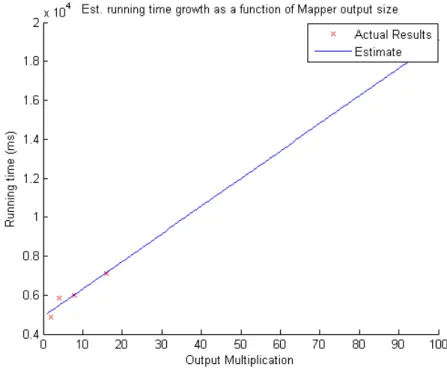
Figure 13: Effect of mapper output on job length

We have then extrapolated the ratio between output multiplication factor and the running time increase that would be required to produce it.

(19)

The map average time equals to (141.7845 ∗ i) + 4891.1, where i is the multiplication factor of the mapper average output size.

Next we have inputted the function into our mathematical model and iterated over different

multiplication factors in order to find if such a tipping point exists and if it does when it does occurs. We have iterated from 1 (no multiplication) to 1,000,000 and no such tipping point occurred. This brought us to the conclusion that for job with a nature such as word count there is no tipping point, i.e. in the map phase the mapper average time will always be bigger than the shuffle time.

Summary

In this paper we aimed to investigate the deployment of a Hadoop cluster in a virtualized data center environment. We have begun by developing a tool that would augment Hadoop's counter metric gathering system in order to gather additional statistics that Hadoop itself does not collect. Using this system, we have been able to evaluate the network performance of a Hadoop

deployment on Amazon and gain insight into the amount of traffic Hadoop generates and the network resources provided by Amazon EC2.

Following this first step, we have discovered that Hadoop's network utilization is low and have decided to try and deploy Hadoop between two data centers connected by the public Internet. This deployment took place on Elastichosts and we can now conclude that unmodified Hadoop code can indeed be deployed in such a cluster.

With the measurements gained from both deployments, we have then created a mathematical model which allows for the approximation of a Hadoop job's runtime. Using this model, we were able to conclude that Hadoop jobs are not, typically, network constrained and even very large (for example, an order of magnitude) increase in mapper output (which is the most significant source of data transfers in a Hadoop job) does not affect running time significantly (or if it does, then the increase of the reducer and mapper running times is still the dominating factor). This is likely our most interesting result, which opens the way to additional research into Hadoop deployments across the Internet and other research testbeds.

(20)

This work has been supported by the LAWA project, an EC collaborative research project (number 258105) on “Longitudinal Analytics of Web Archive Data” which is a part of the FIRE ("Future Internet Research and Experimentation") portfolio of ICT research supported by the EC.

References

[1] Foundation, The Apache Software, "Who Uses Apache Hadoop," 2012. [Online]. Available: http://hadoop.apache.org/who.html.

[2] J. Dean and S. Ghemawat, "MapReduce: Simplified Data Processing on Large

Clusters," in MapReduce: Simplified Data Processing on Large Clusters, ACM, 2008.

[3] Amazon, "Amazon Elastic Compute Cloud (Amazon EC2)," [Online]. Available: http://aws.amazon.com/ec2/.

[4] ElasticHosts, "Elsatichosts Cloud servers," [Online]. Available: http://www.elastichosts.com/.

[5] M. D. Hill, The Datacenter as a Computer, Morgan & Claypool, 2009.

[6] J. Dean and S. Ghemawat, "MapReduce: A Flexible Data Processing Tool," vol. 53, no. 1, 2010.

[7] J. Xie , S. Yin, X. Ruan, Z. Ding, Y. Tian, J. Majors, A. Manzanares and X. Qin, Improving MapReduce Performance through Data Placement in Hetrogeneous Hadoop Clusters, Department of Computer Science and Software Engineering, Auburn University, Auburn, AL.

[8] M. K. Horacio GonzáLez-VéLez, "Performance evaluation of MapReduce using full virtualisation on a departmental cloud," International Journal of Applied Mathematics and Computer Science, vol. 21, no. 2, pp. 275-284, June 2011.

(21)

[9] K. Kambatla, A. Pathak and H. Pucha, "Towards optimizing hadoop provisioning in the cloud.," in Proc. of the First Workshop on Hot Topics in Cloud Computing, 2009.

[10] N. B. Rizvandi, J. Taheri, R. Moraveji and A. Y. Zomaya, "Network Load Analysis and Provisioning of MapReduce Applications," 2012.

[11] A. Greenberg, J. R. Hamilton, N. Jain, S. Kandula, C. Kim, P. Lahiri, D. A. Maltz, P. Patel and S. Sengupta, "VL2: A Scalable and Flexible DataCenter Network," vol. 54, no. 3, 2011.

[12] S. Kandula, S. Sengupta, A. Greenberg, P. Patel and R. Chaiken, "The nature of data center traffic: measurements & analysis," in Proceedings of the 9th ACM SIGCOMM conference on Internet measurement conference, New York, NY, 2009.

[13] M. Al-Fares, S. Radhakrishnan, B. Raghavan, N. Huang and A. Vahdat, "Hedera: dynamic flow scheduling for data center networks," in NSDI'10 Proceedings of the 7th USENIX conference on Networked systems design and implementation, USENIX Association Berkeley, CA, USA, 2010.

[14] K. Church, A. Greenberg and J. Hamilton, "On delivering embarrassingly distributed cloud services," 2008.

[15] Project Gutenberg, "Project Gutenberg," 2013. [Online]. Available: http://www.gutenberg.org/.