copula based bivariate option pricing
by
TORGEIR W. B. HOFFMANN
MASTERTHESIS
for the degree
Master of Science in Modelling and Data
Analysis
(Master of Science)
Det matematisk- naturvitenskapelige fakultet
Universitetet i Oslo
March 2009
Faculty of Mathematics and Natural Sciences University of Oslo
Let me start by thanking my supervisor Fred Espen Benth for providing me with an interesting project. His patience and quick response have been critical to the development of the ideas presented herein.
Varm thanks to Paul C. Kettler. Without his good advice and frequent discus-sions, this thesis may have been very different. I am very grateful for all that he has done.
Last, but not least, I would like to thank my family and friends, who provided me with support when things looked darkest.
March, 2009
Torgeir W. B. Hoffmann
We aim to study how copula based dependence modelling of jump sizes in the NIG-Lévy model affect the option price. This leads to the definition of a rejec-tion based approximarejec-tion algorithm for the NIG-Lévy.
Using small jumps approximation provided by theory from Asmussen and Rosinki, an automatic algorithm is developed. Furthermore, the empirical copula of two dependent processes is extracted and analysed. In general, it can be observed that the small jumps dominate the dependence structure, as well as the behavior of the process. An observation with regards to thin tails is made: The depen-dent jumps produced by the conditional copula distribution vary a lot even in the 4th or 5th significant digit. Therefore, one can see indications that, for certain parameter sets, copulas with sufficient spread in the tails may produce very large jumps in one marginal process, while the other experience very small jumps.
Finally, a discussion on the effect of the copula on option prices is presented, and compared to the option price of independent processes. An approach to finding the Esscher parameters is presented, and the issues using an Esscher transform on dependent processes are presented.
The findings indicate that copulas on large jumps can have a bigger effect on the option prices if dependency is low, as variation in large jumps can be bigger for the dependent process than the original process. For high dependency, the option prices are generally lower than in the independent case, as dependence restrict the movement of the second process.
All simulations were done using R (http://www.r-project.org). Plotting was done using R and gnuplot (http://www.gnuplot.info).
1 Lévy processes, approximation and simulation 1
1.1 Leaving the Black-Scholes world behind . . . 1
1.2 Lévy processes . . . 3
1.3 Approximation of the Lévy processes . . . 6
1.4 Simulation of Lévy processes . . . 8
2 Dependence between Lévy Processes 23 2.1 Conventional measures of dependence . . . 23
2.2 Copulas . . . 24
2.3 Lévy-copulas . . . 29
2.4 Bivariate distributions with NIG marginals . . . 30
2.5 The model . . . 32
2.6 Simulation of dependent NIG-Lévy approximations . . . 33
3 Option pricing with Dependent Lévy processes 39 3.1 Asset price model . . . 39
3.2 Risk Neutral Measures . . . 39
3.3 Option pricing . . . 44
3.4 Concluding remarks . . . 45
4 Conclusion 49 A 51 A.1 Esscher transform for the NIG-Lévy approximation . . . 51
B 53 B.1 Source code: approximation . . . 53
B.2 Source code: copula simulations . . . 63 B.3 Source code: option pricing . . . 66
Lévy processes,
approximation and simulation
1.1
Leaving the Black-Scholes world behind
The Black-Scholes theory was no doubt one of the most important break-throughs in modern mathematical finance. It builds on the assumption that the log-returns for a given risky security follow a Gaussian distribution. While it is easy to model and implement, it lacks flexibility and has tails that are far too light to describe the distributions of observed daily log-returns.
The framework is rather inflexible in view of the restrictions such as constant risk-free interest rate, drift and volatility, the absence of transaction costs, and the assumption that one can buy any quantity of a share, no matter how small. However, these are restrictions that one can argue to be necessary if the math-ematical model is to have some level of simplicity. On the other hand, the model can be fitted with a heavier tailed distribution. This improves the fit to empirically observed data and risk evaluation.
1.1.1
The fat-tails problem
One of the primary concerns of risk management is heavy tails. Clearly, a model that describes more accurately the tails of a distribution of returns will have big impact on the portfolio of an investor or company. If the tails are too light the risk of big losses is underestimated; the losses will occur more frequently and can lead to very grave results indeed. On the other hand, overestimating the risk will lead to funds not being allocated as efficiently as possible, and the investor can miss opportunities of increased returns on his portfolio.
This calls for a more flexible model, which can more accurately capture the behavior observed. Many heavy tailed distributions exist, among them the Cauchy distribution and Pareto. One should remember that the distribution should be flexible enough to capture skrewness as well. The normal inverse
Gaussian is such a distribution.
1.1.2
Normal inverse Gaussian distribution
The NIG distribution is much more flexible than the commonly used Gaussian distribution, and is able to reflect both semi-heavy tails and skewness in the dis-tribution. Semi-heavy tails are in general classified as being heavier than those of the Gaussian distribution, but lighter than those of α-stable distributions such as the Cauchy.
However, this comes at a cost of more parameters. This is not desireable from a modelling point of view. Even if a model fits very well to the observed returns, the cost of modelling and fitting more parameters might be too high compared to the gain. However, the NIG distribution strikes a good balance with four parameters, and a good fit to empirically observed data. While the NIG was in-troduced by Barndorff-Nielsen to model the size of gains of sand, it has proven to have very good fit in several other applications, among them financial markets. See Barndorff-Nielsen [5] and the references therein to Shephard [21].
The distribution function is defined as:
nig(x;α, β, δ, µ) =c·exp{β(x−µ)}K1(αg(·xg(x−µ))
−µ) (1.1)
whereg(x) =√δ2+x2andK
1is the modified Bessel function of 2nd kind order
11 : K1(x) = 1 2 Z ∞ 0 exp{−12x(z+z−1)}dz (1.2)
and the constantc is given as:
c=δα
π exp{δ
p
α2−β2}
Here the parameters of the NIG distribution have the following effect: • α: tail-heaviness/shape
• β: skewness. β >0means skew to the right,β <0left,β = 0symmetric. • δ: scale parameter, similar to variance, controls pointiness of distribution. • µ: location
For the distribution to have the desired qualities we need to put some additional restrictions on the parameters [3, 1.3.32]: α≥ |β| ≥0 andδ >0.
1
Referred to as the modified Bessel function of 3rd kind order 1 by some authors, but this is now less common.
The moment generating function of the NIG is easily derived by simple algebra as:
M(u) =eµu+δ(√α2−β2−√α2−(β+u)2)
This is interesting and will be returned to in Chapter 3, but it should be noted that it has a very simple form. This is useful from a modelling perspective and especially with respect to option pricing since it is easy to work with.
1.2
Lévy processes
Definition 1.2.1(Lévy process).Lévy processes are a special class of stochastic processes with the following properties:
• Stochastically continuous
• Stationary with independent increments
1.2.1
Tail integrals and Lévy measures
From Cont and Tankov [9, 5.7] we have:
Definition 1.2.2 (Tail integral). A d-dimensional tail integral is a function
U : [0,∞]→[0,∞]such that
1. (−1)dU is d-increasing, i.e. ∆x2 x1∆
y2
y1U(x, y)≥0
2. U = 0if one of its arguments is equal to ∞ 3. U is finite almost everywhere,U(0, . . . ,0) =∞
In other words the tail integral has many similarities to the survival probability function, but the former is more generalized. A survival probability is the tail integral of a probability distribution, and the tail integral plays a very specific role with the Lévy measure. From Cont and Tankov [9, 3.4]:
Definition 1.2.3(Lévy measure). Let(Xt)t≥0be a Lévy process onRd. Define
the Lévy measureν onRby:
ν(A) =E[#{t∈[0,1] : ∆Xt= 06 ,∆Xt∈A}], A∈B(R)
Here we can find an interesting connection. The tail integral of the Lévy measure from a pointxis the intensity, or the expected number of jumps with size greater than or equal toxin a unit interval of time. If the Lévy measure is finite, then the intensity is naturally finite everywhere.
1.2.2
Lévy-Itô decomposition
This celebrated result is fundamental when working with Lévy processes, and gives us great insights into the building blocks of the process. Before the theo-rem, a definition is in order:
Definition 1.2.4 (Poisson random measure). Let B0 be all Borel sets not
containing 0. Let the increment of a Lévy process be∆l(t) =l(t)−l(t−). Then
the Poisson random measure ofl(t)is defined as:
N(t, U) = X
s:0≤s≤t
χU(∆l(t))
From Applebaum [3, 2.4.16] the results can now be stated:
Theorem 1.2.5 (The Lévy-Itô decomposition). If X is a Lévy process, then
there exists a∈ Rd, a Brownian motion Bσ with covariance matrix σ and an
independent Poisson random measure N on R+×(Rd\ {0})such that for each
t≥0: Xt=bt+BA(t) + Z |x|<R xN(e t,dx) + Z |x|≥R xN(t,dx)
R can be arbitrary, but it is common to letR= 1.
Here N(e t,dx) = N(t,dx)−tν(x). This compensation is necessary where the intensity of the small jumps is infinite and forN(e t,dx)to be a martingale (See Øksendal and Sulem, 2004).
The triplet(a, σ, ν)is commonly referred to as the Lévy triplet, and consists as above of a drift a, covariance matrixσand a Lévy measureν.
This means that the basic building blocks of a Lévy process is a drift term and a Brownian motion for the continuous part. Furthermore, we have a term for the small jumps and a term for the big jumps.
1.2.3
Lévy-Khinchin
This theorem is a very important since it tells us that the small jumps in the Lévy-Itô decomposition are actually independent of the big jumps.
Theorem 1.2.6 (Lévy-Khinchin). Let Xt be a Lévy process with Lévy triplet
(a, σ, ν). Then
Z
R\{0}
min{x2,1}ν(dx)<∞
E{eiuXt}=etψ (1.3) ψ=aiu+1 2σ 2u2 + Z R\{0} eiux−1−iuxχ|x|<1 ν(dx) (1.4)
This is important from a modelling perspective. It gives an explicit shape for the characteristic function and determines an important relationship between the small and big jumps: independence. This property will be actively used in modelling. It makes it possible for us to model the dependency between the big jumps of two processes without regard to the connection between the small jumps and vise-versa. This relationship can be confirmed using Kac’s theo-rem [3, 1.1.15].
From this we also get useful notation that can be applied to all Lévy processes: the Lévy triplet2
(a, σ, ν), whereais a constant,σis a square matrix and ν is the Lévy measure. This triplet uniquely determines the Lévy process.
1.2.4
NIG-Lévy process
The NIG-Lévy process has its increments distributed as: Xt−s∼nig(α, β, δ(t−
s), µ(t−s)).
From Barndorff-Nielsen [4, 4.11-4.13] we have that the NIG-Lévy process can be represented by a triplet(a,0, ν), where
a=µt+2δtα π Z 1 0 sinh(βx) K1(αx) dx ν(x) = δtα π|x|e −βxK 1(α|x|) (1.5)
Note that the Lévy measure is independent of µ. Important to note is that
from the Lévy triplet we have that our NIG-Lévy process is in fact a pure jump process. In other words it has no continuous part represented by a Brownian motion as indicated by the Lévy-Itô decomposition (1.2.5). This will have con-sequences for our modelling, and in particular for option pricing since a market driven by such processes give rise to an incomplete market. We are dependent on finding a risk neutral probability measure to prevent arbitrage from existing. We will show how to work with this in Chapter 3.
1.2.5
Properties
We will derive some interesting properties of the NIG-Lévy process. For this we will employ several propositions found in Papapantoleon [14]:
Let Xt represent our Lévy process with Lévy measureν(x) given as in (1.5). If ν(R) = ∞, then almost all paths of Xt have an infinite number of jumps
on every compact interval [14, Prop. 7.1]. In that case, the Lévy process has infinite activity. This is easily seen from the form of the Lévy measure. Furthermore, we have that if
Z
|x|≤1|
x|ν(dx) =∞,
then almost all paths have infinite variation [14, Prop. 7.2]. This tells us something about how the small jumps impact on the behaviour of the process, and in particularly that it is dominated by the small jumps. We can also verify this with relative ease as the asymptotic behavior ofK1(x)isK1(x)∼x−1when
x→0. We will look closer at this in our approximation section (1.3), but refer to either Abramowitz and Stegun [1] or Barndorff-Nielsen [4, 4.14] for details. The final property that we will look at is that of moments. If
Z
|x|≥1|
x|pν(dx)<∞
then Xt has finite p-th moment [14, Prop. 7.3]. In our case, this means that
since the Lévy measure has no other atoms, and limx→∞ν(x) = 0 then the
NIG-Lévy process has all moments finite. This is very useful, as it means that one can find expectation and variance. Variance and infinite variation need to be distinguished. While the former is commonly known as the second moment, the property of infinite variation means that at every time interval there is a probability of making large enough moves such that one cannot find an upper or lower bound for the increments on any compact interval.
1.3
Approximation of the Lévy processes
Looking at the possiblities of approximating the NIG-Lévy is of interest, as an opproximation on the form of the Itô-Lévy decomposition will enable modelling of the drift, brownian diffusion, small jumps and large jump independently. This allows for great flexibility, in particular in dependence modelling as will be covered in Chapter 2
From the Barndorff-Nielsen representation of the NIG-Lévy process, and that the integral in the Itô-Lévy decomposition can be approximated by a compound Poisson process where the intensity of the jumps are given by the integral of the Lévy measure over its entire support.
This leads to the following expression for the NIG-Lévy using the notation from (1.5): L(t) =at+ N X i=1 (t)γ(t)
However, it should be noticed that the NIG-Lévy as mentioned has infinite activity in the origin, and hence the theoretical intensity of the Possion process,
N(t), is infinite. For the small jumps, it is therefore necessary to take some extra precautions.
1.3.1
Approximation of the jump size distribution
One approach is to approximate the jump size distribution. The idea is simple: In many cases the Lévy measure is finite, and hence:
K=
Z
R
ν(dx)<∞
Therefore, we can define the probability measure of a jump,J, as:
P(J ∈U) =ν(U)
K , U ⊂R
From this, one can in theory simulate the jumps of a Lévy process. Combined with the power of the Lévy-Itô decomposition, the process has a complete rep-resentation.
In general, however, a direct simulation in this way contains several pitfalls. As outlined in 1.2.5 our NIG-Lévy process has infinite activity, so that a direct normalization is not possible.
Define small jumps as increments which lie in the interval(−, ). Jumps outside this interval are considered large jumps. One possibility is simply to remove the small jumps, but in our case Barndorff-Nielsen shows that the small jumps are actually dominating the movement of the process. The result is due to a series representation of the process, and the rate at which it goes to infinity near the origin. Since the process has sufficient mass near the origin, it can be approximated.
Approximation of jumps smaller then
Instead of removing the small jumps of sizeor less, Asmussen and Rosinski[20] propose to incorporate their contribution by a Brownian motion with the fol-lowing mean and variance:
µ:=− Z ≤|x|≤1 x ν(dx), σ2() := Z |x|< x2ν(dx) (1.6)
The Brownian approximation of small jumps exploits the result that expected value of the small jumps divided byσ2()converges in distribution to a standard Brownian motion. For details, see the original article referenced above.
One interesting part to note is that even if the process is a pure jump process, the approximation still gives a Brownian part. The result is valid for the NIG-Lévy process [20, Prop. 2.2]. For all practical purposes we will not be able to
distinguish between the small movements of such a Brownian motion and that of a NIG-Lévy process. The error of this approximation will be dealt with in Section 1.4.1.
Dealing with jumps larger than
Since the small jumps are now dealt with, we truncate the Lévy measure in a small neighbourhood of the origin (−, ), and since the Lévy measure of the NIG-Lévy has no other atoms, the normalization constant is finite, even if it’s still not known. Hence it would be possible to simulate the jumps directly
from the the normalized truncated Lévy measure, ν(x), if we can find the
normalizing constant. The constant is not hard to find numerically, but can be quite a challenge analytically. The normalizing constant, from here on referred to asK, is given as: K= Z <|x|<∞ ν(dx) = Z <|x|<∞ δα π|x|e −βxK 1(α|x|) d(x)
Using a Lévy measure truncated around the origin one can avoid discretizing the measure, and hence keep the advantage of the heavy tails. In other words, theoretically one can have draws from the entire support of the jump probability measure, and the only limitation would be that of the computer hardware used for simulation.
Intensity of jumps larger than
In the general case, the itensity of the jumps are equal to the normalization term in the NIG-Lévy jump measure. This is also the case here where the intensity
λis such that: λ=ν((−∞,−]∪[,∞)).
The number of jumps in the compound Poisson process are distributed by a Poisson random variable with the intensityλgiven above. The waiting time be-tween each jump is exponentially distributed [9, Def. 2.17]. The increasing sum of exponentially distributed random variables follows a Dirichlet distributed. This can be simulated using a sorted set of uniform draws on [0, T]. For more information on this, see Cont and Tankov [9, Prop. 2.10]
Note that the larger jumps are not intended to be approximated. Since the intensity is finite direct or indirect simulation is preferred.
1.4
Simulation of Lévy processes
The expressions for the mean and variance of the Brownian part given in (1.6) are finite integrals that we can easily estimate numerically by employing Rie-mann integration with a sufficient discretization, or any other optimized inte-gration method in our software.
To draw the large jumps directly using a pseudo-inverse method is not desirable since one cannot easily invert the modified Bessel functionK1analytically, even
if K1 is strictly decreasing and C1. A search algorithm (e.g., bisection) on a
spline would be inaccurate unless one chooses a large number of knots. In ad-dition, a spline on an unbounded domain will be difficult to implement without imposing artificial boundaries. For high intensity, this method can become very inefficient.
From the definition of the tail integral of the truncated Lévy measure,ν
lim
x→∞ν
(x) = 0
Therefore, it is at least bounded as there are no other atoms save the one in the origin. A function that dominates it on this interval can be found. We can find the asymptotes for our Lévy measure by studying the asymptotes of the Bessel function given in Abramowitz & Stegun[1, 9.6.9] and Barndorff-Nielsen[4, 5.1] repectively: ν(x)∼ δ πx2, x→0 + orx→0− ν(x)∼δ r α 2π|x|3 ·exp{βx−α|x|}, x→ ±∞
We will employ a rejection based sampling methods to draw from our distribu-tion. Using conventional rejection sampling one would need to know either the normalizing constant or at least an upper bound for it3
. Metropolis-Hastings algorithm, on the other hand, does not require the normalizing constant to be known. Another very appealing feature of the rejection based algorithms is that one can avoid the inversion method described above completely. Two algorithms are presented.
The Accept-Reject algorithm
The first algorithm presented is the conventional Accept-Reject method. It is based on the idea that the height of the proposal distribution, q(x), and that of the target distribution, π(x), is compared for each draw proposed. If the proposal distribution has a lot more mass than the target for a a jump, then there is only a low chance that the jump is accepted as a draw. However, if the distributions resembles one another for some areas in the support chance of acceptance in those regions is higher.
Defineαas
α= π(y)
cq(y) 3
Hogstad and Omre, A comparison of Rejection Sampling and Metropolis-Hastings Algo-rithm.
wherey is the proposal drawn and cis a majorizing constant such that
π(y)≤cq(y), ∀y∈suppπ
Since α∈ [0,1], the algorithm rejects with probability 1−α. If rejected, the previous jump is kept. Clearly, the chain of accepted draws determines a random
walk with a move probability ofα. The question that springs to mind is the
rate of convergence to target distribution. As can be seen, the algorithm does not take into consideration anything else, save the height of the distributions. Potentially, this could make the rate of convergence slow.
It is critical that one can find a constant c such that the proposal distribu-tion dominates the target over the entire support. Otherwise, areas may be undersampled and one can end up with automatic acceptance in others since
α= 1. This can lead to extreme undersampling in parts of or the whole target distribution. Still, this may not be enough as some distributions are simply to light tailed to be used efficiently as proposal distributions in some cases. For example, it is very difficult to sample a Cauchy distribution using a Gaussian distribution as proposal because of the light tails in the latter. The converse, on the other hand, works very well.
In addition, it is necessary to know the target distributions normalization factor, or at least an upper bound for it. If not, one cannot guarantee that ac can be found that will allow for optimal convergence of draws to target distribution. However, there are algorithms that can get around these restrictions, and this is particularly useful for high-dimension problems where the normalization con-stant is very computationally demanding.
Provided under results, Table 1.2 compares draws generated through the Accept-Reject algorithm with those of a real NIG-Lévy simulation. The results also cover different proposal distributions.
Metropolis-Hastings algorithm
The second rejection based algorithm presented is the Metropolis-Hastings al-gorithm, which by the construction of a Markov chain can be used to draw realizations of our target distribution ,π(x), which is the normalized truncated
Lévy measure of our NIG process. Letq(x) denote the proposal distribution.
We here employ the same notation as in the excellent paper by Chib and Green-berg [8], but we only consider proposal distributions which are independent of the previous jump. Hence, if two draws are made from q(x): x1 and x2 then
the probability mass of x2 would beq(x2). This is slightly different from the
original algorithm by Hastings, where the law of the second jump depended on that of the first, hence the Markov chain description. The algorithm is given in Algorithm 1.4.1.
The algorithm is rather simple and evolves around the relative mass (or height of probability distribution) of two draws. The acceptance probability,α, is defined as the fraction of the relative mass in the proposal distribution,q(x), andπ(x):
α(x1, x2) = min
1,π(x2)q(x1) π(x1)q(x2)
As can be seen, a higher acceptance probability is given if the shape ofq(x)is close to that ofπ(x). Furthermore, if the target distribution is continuous and differentiable then one would benefit slightly from using a proposal distribution with these properties compared to a discontinuous one.
On the other hand, if no proposal distribution with good shape is available , one can instead choose a mixture of continuous functions which fit well on mutually disjoint sets in the support ofπ(x)as long as the support of the mixture contains that of the target distribution.
This will of course only help on accept probabilities of jumps between these
ar-eas, andαmight still be small for jumps from the same continuous area.
How-ever, since Metropolis-Hastings is much more dependent on the overall shape of the distribution, one can be severely punished for choosing a proposal distribu-tion with poor fit. This can in general lead to very slow convergence due to low rates of acceptance.
Algorithm 1.4.1(Metropolis-Hastings).
1: procedureMetropolis-Hastings(π,F, N)
2: Drawy from F
3: forn≤N do
4: Drawxfrom F andufrom U(0,1)
5: Define: α= ( minππ((xy)F()F(xy)),1 , π(y)F(x)>0 1 ,otherwise 6: if u < αthen 7: Sety=x 8: end if 9: end for 10: end procedure
In general, one can refer to a Markov Chain generated by the Metropolis-Hastings as running too cold or too hot depending on whether the proposal distribution is too heavy or too light in the tails respectively. If the chain runs too cold then the fractionq(x2)/q(x1)will be close to one. If the tails are much
heavier in the target distribution, this will result in a high number of rejections in the tails, and undersampling of high probability areas. An illustration of the under and oversampling for two Gaussian distributions are given in Figure 1.1. Vise versa, if the proposal distribution runs too hot it will too often propose draws from high probability areas. It can therefore take a long time for the chain to traverse the support ofπ(x).
Either of these situations can lead to chain converging slowly to a draw from the target distribution. Furthermore, in both these cases high autocorrelation is likely over the values sampled at the end of each chain[8].
0 0.05 0.1 0.15 0.2 0.25 0.3 0.35 0.4 −6 −4 −2 0 2 4 6 Sampling via Metropolis−Hastings
Target Distribution Proposal Distribution Undersampled points Oversampled points Draws always accepted
Figure 1.1: Illustration of sampling via Metropolis-Hastings
It is important that the support of the proposal is such that: supp(π)⊆supp(q)
If the support of the target distribution is not connected one must ensure that the proposal distribution can at least simulate from the the whole support such that the chain can make the transition from one state to another state in an unconnected part of the support. If this is not possible one may experience mixing problems in the accepted draws.
Clearly, the Metropolis-Hastings algorithm comes at a tradeoff. When using proposal functions with imperfect fit it is highly likely that some areas will be undersampled to some degree or oversampled. Rejection-based algorithms compensate for this run running an increased number of iterations to ensure a good convergence. This is by many still considered an open question although some work has been done in the area, in particular by Raftery and Lewis [15, 16]. A small analysis on this is presented in Section 1.4.3.
In general the chain of accepted draws will be dependent, and therefore we can in principle only use one realization from each chain as an i.i.d. sample [19, p. 234]. This does only in minor degree affect the computational efficiency of our algorithm since few things need to be reinitialized on each run.
Implementation of rejection schemes
The implementation that is quite close to that proposed by Asmussen, Rasmus and Wiktorsson[6]. To analyse the efficiency of the algorithms, two proposal
distributionsJ(x),J1(x)are chosen. They are probability mixtures as follows: J(x)∼ ( wq·fq , x∈[−ω,−]∪[ω, ] we·fe , x∈(−∞,−ω)∪(ω,∞) (1.7) J1(x)∼ ( wq·fl , x∈[−ω,−]∪[ω, ] we·fe , x∈(−∞,−ω)∪(ω,∞) (1.8)
We will onwards refer to J(x) as the inverse quadratic case, and J1(x) as the
inverse linear case. The distribution functions are given as:
fe∼(α− |β|) exp(−(α− |β|)|x−ω|) fq ∼ 1 − 1 ω −1 1 x2 fl∼log ω 1 x
These can very easily be inverted for simulation. Figure 1.2 illustrates two possible setups with the proposal functions given above. The inverse quadratic distribution and Laplace distribution4
have weights wq, we respectively. The weight for the inverse linear,fl, is the same as the former. These can be chosen to be the intensity of the Lévy measure over respective intervals:
we= Z −ω −∞ ν(x) dx+ Z ∞ ω ν(x) dx ·K−1 wq= Z |x|∈[,ω] ν(x) dx ! ·K−1
Note that manual tuning of the weights is not necessary. In particular, ifJ(x) is used as a proposal function, these weights are almost natural due to the very small spread. However, with a looser fit in the proposal function as is the case withJ1(x)proposal function, manual tuning might be necessary due to poor fit
in the tails. However, such manual tuning will only result in less draws from the high probability areas of the proposal, and may in many cases then lead to undersampling. Therefore, the same weight is used in both cases.
As for choosing the truncation levelsandω we will deal with this in (1.4.1). Furthermore, one is free to use a set of scaling constantsc1, . . . , c4 to increase
the acceptance rate. We choose the constants to be such that the proposal distribution is at least continuous:
0 0.2 0.4 0.6 0.8 1 −1.5ω 0 ω 1.5 y x
Lévy measure and inverse quadratic proposal function
Proposal function NIG Lévy measure
0 0.2 0.4 0.6 0.8 1 −1.5ω 0 ω 1.5 y x
Lévy measure and inverse linear proposal function
Proposal function NIG Lévy measure
Figure 1.2: The NIG Lévy measure with proposal functions
0.004 0.006 0.008 0.01 0.012 0.014 0.016 0.018 0.02 0.1 0.12 0.14 0.16 0.18 0.2 y x
Lévy measure and inverse quadratic proposal function
Proposal function NIG Lévy measure
Figure 1.3: A close up look at the NIG Lévy measure with inverse quadratic proposal
c3=δ·α
c4=
c3·fq(ω)
fe(ω)
The constants for the negative half-line can be chosen in similar manner using
the negative truncation point −ω. This can have some effect on the
accep-tance rate for jumps drawn from the Laplace area of the proposal. This can benefit both rejection algorithms. Note thatc3 has as the main purpose to
en-sure domination of the Lévy meaen-sure in the Accept-Reject case, and hence the Metropolis-Hastings will not benefit from this.
On optimal acceptance rates in Accept-Reject
While acceptance rates are not expected to be high when usingJ1(x), they can
be extremely high due to very small spread between the Lévy measure andJ(x). As long asJ(x)can adequately sample the entire support of the Lévy measure, there should not be much of an issue.
One should keep in mind that high accept rates in other cases may not be optimal. Roberts, Gelman and Gilks (1994) showed theoretically that if both proposal and target densities are Gaussian, the scale of the former should be tuned such that the rate of acceptance is0.45in the one-dimensional case and 0.23for dimensions over one. However, for the scope of this thesis, and keeping in mind the very nice shape of J(x) there is little to indicate that maximum acceptance rate is bad.
1.4.1
Accuracy of Approximation
There are two quantities that are of particular interest when we use this ap-proximation of the NIG-Lévy process. First, how good the apap-proximation is. Second, how computationally intensive the approximation is. IfXis the trun-cated process, define the measure of accuracy fort= 1 as:
D() = sup
x∈R|P
(X(1)≤x)−P(X(1)≤x)|
While the details are in Asmussen and Rosinski[20], it can then be showed that this has an upper bound has follows
D()≤(0.7975)σ−3()
Z
|x|<|
x|3Q(dx)
With this upper bound for the error, the truncation level can be chosen based on maximum acceptable error. Given the shape of the Lévy measure of the NIG, it can be very computationally intensive if we choose a truncation level too small. Or vise versa it will not be very accurate if the Brownian motion is
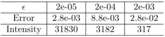
2e-05 2e-04 2e-03
Error 2.8e-03 8.8e-03 2.8e-02
Intensity 31830 3182 317
Table 1.1: Maximum Error Levels of Brownian approximation
left to do most of the jumps. Letδ() =D()/(0.7975). Then for the NIG case we have [20, Theorem 3.1]:
δ()∼
r
π
8δ ·
Using this we can see the maximum error level for some selected values of ,
givenδ= 1is as in Table 1.1. One should also notice that the intensity of the jumps for the chosen values are proportional to the value of , the error level is not. The choice of truncation level also needs to take into consideration the computational effort required.
Clearly from the formula, with highδwe can choose a biggerand thus lower the computational effort required as the intensity decreases. The errors calculated are the maximum, and hence we can expect the approximation to perform better than this much of the time.
From this we can simply invert the above formula for the error of the Brownian
approximation and thuscan automatically be set using the formula:
=8δ
2()·δ
π (1.9)
For the second truncation there is a slightly different approach. The first thing that should be observed is that fq is lighter in the tails than the target Lévy measure for some values ofαandβ. Hence it will at some point cross the graph
of the Lévy measure. There is a possibility of undersampling if ω is chosen
too large. On the other hand, choosing ω too small will result in inefficient
sampling, as the second term in the proposal,fehas very poor resemblence to the normalized Lévy near the origin. This in turn leads to poor acceptance rates, and slow convergence.
However, the following equation uniquely determines ω, and furthermore this
solution forω maximizes the acceptance rate. It is based on the method of S.
Rasmus [18, Theorem 3.2], but differ due to using a simpler proposal function
since fe in this case is symmetric around the origin. This will simplify the
solution by quite a bit compared to the one referred.
Proposition 1.4.2. The value ofω that maximizes the accept probability in the Accept-Reject algorithm solves the equation:
βS(ω)−ω2C(ω)−α ω |ω| K0(α|ω|) K1(α|ω|) C(ω) =−(α+|β|) ω 2 C() (1.10)
where
S(ω) = sinh(βω)K1(αω)
ω , C(ω) =
cosh(βω)K1(αω)
ω
Proof. Define the majorizing contantcsuch thatπ(x)≤cq(x). Writecin term
ofω as: c(ω) = ν (−ω) fe(ω) + ν(−) fq() + ν() fq()+ ν(ω) fe(ω) = ν (−ω) +ν(ω) α+|β| + ν(−) +ν() fq()
The aim is to findc(ω)such that the sum of fractions is as big as possible with the above restriction. Differenciate w.r.t toω:
c0(ω) =∂ων (ω) α+|β| + ∂ων(−ω) α+|β| −(ν () +ν( −))∂ωfq() fq()2 where ∂ων(ω) = β−ω2 −α ω |ω| K0(α|ω|) K1(α|x|) ν(ω) ∂ωfq() =− ω 2 fq()2
Exploiting the following relationship between S(ω), C(ω) and ν(ω) [18, A.5, A.6]: ν(ω)−ν(−ω) = 2δα πK sinh(βω)K1(αω ω ν(ω) +ν(ω) = 2δα πK cosh(βω)K1(αω ω
Substitution for the above expressions:
4δα πK c0(ω)(α+|β|) = β−ω2 −α ω |ω| K0(α|ω|) K1(α|x|) (S(ω) + C(ω)) + β+ 2 ω +α ω |ω| K0(α|ω|) K1(α|x|) (S(ω)−C(ω)) + 2C() ω 2 (α+|β|)
Simplifying the above expression and settingc0(ω) = 0gives the desired
A similar calculation can be done in the inverse linear case, but the equation is somewhat more complex since fl has a different partial derivative w.r.t. ω:
∂ωfl6=−C·fl2. Furhtermore, this choice forω is valid for both the Metropolis-Hastings as well as for the Accept-Reject algorithm, as the majorizing constant will simply be eliminated in the former due to the fraction. However, the choice forω may be bigger in the case ofJ1(x)owing to a lower derivative.
As can be noticed, theαandβare the ones that influences the second truncation
ωthe most of the NIG-parameters. This is expected, asδandµhave little effect on the tails themselves.
1.4.2
Implementation issues
Some issues did come up during implementation. In particular, when imple-menting programmatically it is difficult to determine exactly in which interval a solution to Equation 1.10 exists. This is necessary for solving the equation numerically. Some initial tests showed that the solution was approximately in-versely proportional to the value ofαtimes a constant. The choice was therefore made to search in the interval between and 15·α−1. For extreme values of
α, manual tuning may be necessary, but this is a programmatic concern, and
therefore it has not been analysed further.
There were no other implementation issues worth mentioning, but it should be noted that the algorithm is rather heavy computationally for large numbers of jumps. Large quanta of high speed memory are therefore recommended for efficient simulation.
1.4.3
Simulation of the normal inverse Gaussian
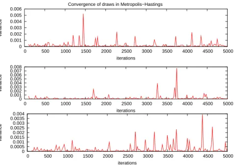
The first issue to deal with in Markov Chain Monte Carlo is the number of iterations required for convergence. As suggested by Raftery and Lewis [15], a small analysis on sample variance is performed.
A method of determining how many iterations the chain must take to produce a valid draw is to study the variance of the draws as the number of iterations is increased. This can be a time-consuming job, but it can give an indication on the minimum of iterations required. Results from 3 independent runs are available in Figure 1.4.
In all of them, the algorithm shows very good rates of convergence, and simu-lation indicates that one can get away with as few as 500–1000 iterations. This can greatly decrease computation time when generating huge number of draws. The following plot shows a sample simulation of the approximation via Metropolis-Hastings compared with that of a NIG-Lévy process with the same parameters. As can be observed in Figure 1.5, the simulations have similar range and from a first look seems similar.
Convergence of draws in Metropolis−Hastings 0 0.001 0.002 0.003 0.004 0.005 0.006 0 500 1000 1500 2000 2500 3000 3500 4000 4500 5000 variance iterations 0 0.001 0.002 0.003 0.004 0.005 0.006 0.007 0.008 0 500 1000 1500 2000 2500 3000 3500 4000 4500 5000 variance iterations 0 0.0005 0.001 0.0015 0.002 0.0025 0.003 0.0035 0.004 0 500 1000 1500 2000 2500 3000 3500 4000 4500 5000 variance iterations
Figure 1.4: Variance from 3 random starting points simulations via Metropolis-Hastings.
Simulation of NIG−Levy vs approximation
−0.3 −0.2 −0.1 0 0.1 0.2 0.3 0.4 0.5 0 0.2 0.4 0.6 0.8 1 Approximation of NiG−Levy via M−H
−0.9 −0.8 −0.7 −0.6 −0.5 −0.4 −0.3 −0.2 −0.1 0 0.1 0 0.2 0.4 0.6 0.8 1 Simulation of NiG−Levy
M-H A-R NIG-Levy
x−1 x−2 x−1 x−2
#(J>) 2445 2235 2368 2273 2388
Accept % 0.5001 0.9997 0.05818 0.9997
-mean(J) -3.99e-02 8.09e-06 6.31e-04 6.74e-05 3.92e-05
var(J) 2.76e-02 6.27e-05 2.09e-04 4.56e-05 1.67e-05
mean(|J|>) -1.63e-01 2.89e-05 2.65e-03 2.96e-04 2.19e-04
var(|J|>) 9.28e-02 2.8e-04 8.8e-04 2e-04 1.72e-04
Table 1.2: Statistics for approximations and NIG-Lévy simulation
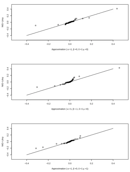
−0.4 −0.2 0.0 0.2 0.4 −0.4 −0.2 0.0 0.2 0.4 Approximation ( α =1, β =0, δ =1 µ =0) NIG−Lévy −0.4 −0.2 0.0 0.2 0.4 −0.4 −0.2 0.0 0.2 0.4 Approximation ( α =1, β =.1, δ =1 µ =0) NIG−Lévy −0.4 −0.2 0.0 0.2 0.4 −0.4 −0.2 0.0 0.2 0.4 Approximation ( α =1, β =0, δ =1 µ =1) NIG−Lévy
results compared to a simulation directly from NIG-Lévy. However, one should
notice that these simulations were done under specific conditions. First, ω
was fixed to1.38, but this is mainly to see how the different proposals perform under similar conditions. Furthermore, for simulations in Table 1.2 the following parameters were chosen for one time step, where each time step has 10000 points in the simulation grid: α = 1, β = 0, µ = 0, δ = 1. The accept rates and other statistics using both proposal functions were compared against each other, and all simulations where done with 1500 iterations in the rejection based algorithms. It can be confirmed that the approximation works well by looking at the quantile-quantile plots for different parameters. From the results in Figure 1.6 one can observe that the approximation does quite well. For some outliers it may merely depend on the specific run, as the heavy tails can cause some results to be off, and there is also a small contribution in the error by the Brownian approximation of the small jumps.
Both methods performed very well with thefq as part of the proposal, yielding over 99% acceptance rate on average. While this in general situations could be a reason for concern, it is natural in this setting as the spread between the proposal and the target density is very small. Usingflas a part of the proposal on the other hand did not produce very convincing results. As can be expected from Figure 1.2, using this proposal would lead to very slow convergence, and there are some signs of this in the results when comparing to the results produced by the NIG-Lévy process and the theoretical values.
All in all, the approximation seem to work very well, and there is some indica-tions that Metropolis-Hastings with a proposal includingfq will produce very satisfying results with fast convergence. This is therefore the preferred method of choice in the chapters that follow. Although it will be stated explicitly which parameters are used, we can already here say that one can run Metropolis-Hastings for less than 500 iterations and still get good approximations.
Dependence between Lévy
Processes
The study of dependence between stochastic processes has a long history in statistics, from the use of simple bivariate distributions which share some com-mon parameters, to non-linear measures of dependence and measures of concor-dance.
This chapter extends the previous chapter by introducing dependence between the jumps in NIG-Lévy approximations. Restricting the model to two dimen-sions, the effect of dependence between the small jumps and dependence between large jumps is studied.
2.1
Conventional measures of dependence
The most known and commonly used tool employed in modelling dependence is the correlation, relating to Pearson’s product-moment correlation coefficient,
ρ. This is defined as
corr(X, Y) = pcovar(X, Y)
var(X)var(Y)
In this thesis, the term correlation is reserved for this particular linear depen-dence measure. In general the term dependepen-dence will be used, while some mea-sures are referred to as meamea-sures of concordance. The latter do not in the same way measure the dependence, but focus on the probability of joint movements
up or down. Two famous examples are Kendall’sτ and Spearman’sρs. In this
thesis, however, the connection between these and the dependency structure, copulas, is not in focus. More information on this connection can be found in Frees and Valdez [10, Table 3], or for an introduction, see Nelsen [13, 5.1.1,5.1.2].
2.2
Copulas
Copulas are not a new concept; they were first introduced by Sklar (1959). However, there has been significant progress in the field, especially from a prac-titioner’s point of view. With the ultimate goal to make as good a model as possible fitted to market data, the concept of dependence is even more central than before, especially when looking at structured products (e.g. derivatives) that cover more than one underlying.
Definition 2.2.1(Copula). A 2-dimensional copula is a functionC: [0,1]2→
[0,1]such that:
• C is grounded, i.e. C(x, y) = 0ifx·y= 0 • C is 2-increasing
• ∀(x, y)∈dom(C)we haveC(u,1) =uandC(1, v) =v
Furthermore, if the copula satisfies certain smoothness conditions, the copula density is given as:
C(U =u, V =v) =∂C(u, v)
∂u∂v
The existence of the copula density can in some cases become vital for simu-lation. To understand the flexibility and power that can be gained by using copulas for dependence structure, Sklar’s famous result must be introduced.
2.2.1
Sklar’s Theorem
Theorem 2.2.2 (Sklar’s Theorem). Let C be a copula, andF andGmargins.
Let H be a multivariate density. Then
H(x, y) =C(F(x), G(y)) (2.1)
If F andGare continuous, thenC is unique. Conversely, given a multivariate
distributionH and marginsF andG, there exists a copula such that (2.1) holds.
Again, ifF andG are continuous, thenC is unique.
The result is a very elegant, and shows that copulas can be used to model the dependence independently from the margins. This gives a whole different kind of flexibility compared to the linear correlation. For example, one can keep the dependence structure constant, while changing all or a few of the margins of the underlyings.
Furthermore, it follows that there is an equally interesting relationship that will be very useful in studying how the overall copula changes when the processes are a mixture of several multivariate distributions each with their own dependence structure.
2.2.2
Archimedean copulas
This particular class of copulas is worth special attention. They have a structure that make them easy to work with and extend over several dimensions. In common they have that they can be written in terms of a generator function.
Definition 2.2.3 (Generator function of a copula). The (additive) generator function of a copula,φ(x), is a strictly decreasing function such that:
C(u1, . . . , un) =φ−1( n
X
i=1
φ(ui))
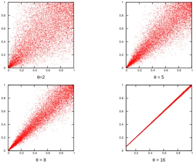
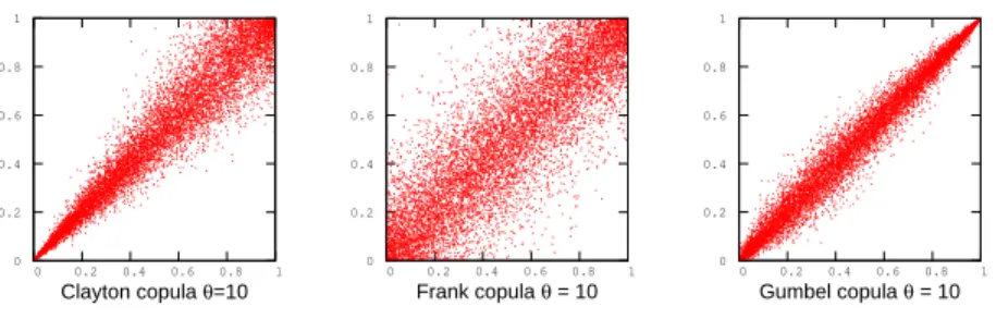
All copulas of the Archimedean class have the property that they can be written in terms of their generator function and its inverse [13, theorem 4.1.4]. This will be a very useful fact in simulation with copulas. It should also be noted that a copula of Archimedean class is symmetric with repect to its arguments. In this thesis the copulas Clayton, Frank and Gumbel are studied, and sample pairs generated from these copulas are presented in Figure 2.2.
Clayton copula
Definition 2.2.4 (Clayton family). A one parameter family of copulas given as:
C(u, v;θ) = u−θ+v−θ−1−1/θ, θ >−1
The copula is asymmetric with higher dependence in the lower tail than in the upper. The parameter of this family controls the dependence in the lower tail,
and the higher the θ is, the higher the dependence. For the limiting case of
θ→0the copula is the indepence copula.
An example with different parameters is given in Figure 2.1.
Frank copula
Definition 2.2.5(Frank family). A symmetric one-parameter copula given as:
C(u, v;θ) =−1 θlog 1 +(e −θu−1)(e−θv−1) e−θ−1
The copula is symmetric around the point (1/2, 1/2), and hence any change in the parameterθwill influence dependence in the tails equally.
Gumbel copula
Definition 2.2.6(Gumbel family). An asymmetric one-parameter copula given as:
The Gumbel has more dependence in the upper tail than in the lower, but it does not have the same spread as the Clayton. This makes it very suitable for problems where the dependence relationship is asymmetric, but still has high dependence in both tails.
0 0.2 0.4 0.6 0.8 1 0 0.2 0.4 0.6 0.8 1 θ=2 0 0.2 0.4 0.6 0.8 1 0 0.2 0.4 0.6 0.8 1 θ = 5 0 0.2 0.4 0.6 0.8 1 0 0.2 0.4 0.6 0.8 1 θ = 8 0 0.2 0.4 0.6 0.8 1 0.2 0.4 0.6 0.8 1 θ = 16
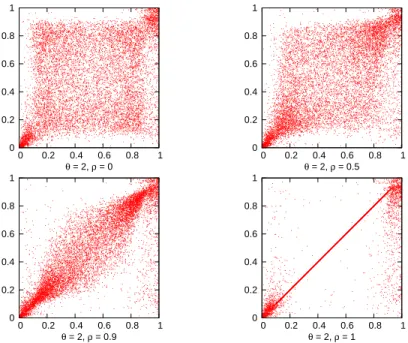
Figure 2.1: Simulation of the Clayton copula with differentθ
2.2.3
Simulation via copulas
The presented methods are more concisely described by other authors, for ex-ample Frees and Valdez [10]. The two methods which will be employed in the simulations are the following:
First, the conditional law of a copula is given by the following expression as long as the copula is smooth enough to be differentiable:
dC(u, v)
du =P(V ≤v|U =u)
This conditional law is one of the very basic tools that can be employed in order to simulate a pair of dependent processes. A basic algorithm will look like the following:
Algorithm 2.2.7(Simulation of dependent pair using conditional law).
1: Letua be value of the first process’ CDF. 2: Draw V1 fromU(0,1)
3: Define vas: v= dC(u, v) du −1 V1 return(u, v)
0 0.2 0.4 0.6 0.8 1 0 0.2 0.4 0.6 0.8 1 Clayton copula θ=10 0 0.2 0.4 0.6 0.8 1 0 0.2 0.4 0.6 0.8 1 Frank copula θ = 10 0 0.2 0.4 0.6 0.8 1 0 0.2 0.4 0.6 0.8 1 Gumbel copula θ = 10
Figure 2.2: Simulation of Clayton, Frank and Gumbel copula
A second approach to simulating from a copula is through its generator. This method generates a pair of dependent variables, but it can be modified to gen-erate a second dependent variable given the first. Exploiting the relationship between the inverse of the generator and Laplace transform for common dis-tributions gives rise to the following algorithm first mentioned in Marshall and Olkin (1988), and employed by Frees and Valdez [10] among others:
Algorithm 2.2.8(Simulation through inverse generators).
1: Simulate a variateX where the Laplace transform of the distribution func-tion is equal to the inverse of the generator,φ−1.
2: Simulate two independent variateV1, V2∼U(0,1).
3: Define:
u=φ−1(−log(V1)/X), v =φ−1(−log(V1)/X)
return(u,v)
Clayton copula
The Clayton copula has a simple structure and is easy to simulate through Algorithm 2.2.7 since it is easy to differentiate and invert:
dC(u, v) du =−θ
−1(u−θ+v−θ−1)−(1/θ)−1(−θ)u−θ−1
Inverting aroundV1∼U(0,1)through simple algebra, the resulting conditional
v= (uθy−θ/(θ+1)+uθ−1)1/θ
It should be noted that since Clayton is an Archimedean copula, it could equally well be simulated via Algorithm 2.2.8. On the other hand, there is no reason to apply a more sophisticated method when it can easily be differentiated and inverted.
Gumbel copula
The Gumbel copula on the other hand can be simulated from using the second
method. Let the single parameter of the Gumbel be θ. The inverse of its
generator function is the Laplace transform of positive stable variate [10, Table 2] with the following parameters:
α= 1/θ, β= 1, γ= (cos(π/(2θ)))θ, δ= 0
Hence, ify∼St(α, β, γ, δ), and u∼U(0,1)then calculate:
v= exp
−log(XV2)
The pair (u, v) is then a realization from the Gumbel copula. However, in
applications where one dependent draw is generated from another draw, one already have one realization from the jumps. Therefore, one can choose which variable one is interested in simulating, and which one that should be calculated
based on the first draw. Choosing V1 to be the drawn variable in Algorithm
2.2.8,X can be calculated as:
X = −log(V1) (−log(u))θ
A dependentv is found by substitution in the expression given above.
Frank copula
Similarly to the Gumbel, the Frank copula can be simulated using the second method. Here the inverse of the generator function is the Laplace transform of a logarithmic series distribution on the positive integers [10, Table 2]. However, the distribution is not implemented in software directly, nor did Frees and Valdez give the required argument.
Fortunately, using the same methods as with the Gumbel copula one can avoid the simulating from the logarithmic series distribution, and simply draw a ran-dom standard uniform number. Ifuis the first random number drawn, andV1is
as in Algorithm 2.2.8, then the following gives the second dependent realization:
where
X= log(V1)
log(e−θu−1)−log(e−θ−1), V1, V2∼U(0,1)
2.3
Lévy-copulas
While the concept of conventional copulas is well-explored and documented, they do not guarantee that structure is preserved. In other words, it is not clear in general if the resulting measure of a Lévy process passed through a copula will produce another Lévy process. However, there are examples of this. Most known is the Gaussian copula joining two Brownian motions, which produces a 2-dimensional Brownian motion. However, this is not the case for any other copula joining two Brownian motions. This issue calls for somewhat similar, but different concept.
Tankov defines an equivalent concept for Lévy processes named not surprisingly Lévy copulas [9, Def. 5.12]. They share many properties with conventional copulas.
Definition 2.3.1(Lévy copula). A functionF(x, y) : [−∞,∞]2→[−∞,∞]is
a 2-dimensional Lévy copula if: • F is 2-increasing
• F(0, x) =F(x,0) = 0,∀x
• F(x,∞)−F(x,−∞) =F(∞, x)−F(−∞, x) =x
As can be seen, they do not share the domain or range with conventional copulas since they act on the tail integral of the Lévy measure and not the CDF of the probability measure. Since the Lévy measure contains all the information of the stochastic jump behavior of the Lévy process, one is guaranteed that a Lévy process is the result when joining two Lévy processes with a Lévy copula.
2.3.1
Sklar’s Theorem for Lévy copulas
From Cont and Tankov [9, theorem 5.6] there exist a similar result to Sklar’s Theorem for Lévy copulas:
Theorem 2.3.2(Sklar’s Theorem for Lévy copulas). LetUbe an d-dimensional tail integral for a d-dimensional Lévy process with positive jumps. Furthermore,
U1, . . . , Ud be tail integrals for one-dimensional Lévy processes. Then there exist
a Lévy copulaF such that
U(x1, . . . , xd) =F(U1(x1), . . . , Ud(xd))
IfU1, . . . , Udare continuous then F is unique, otherwise it is unique onRanU1×
Conversely, if F is a d-dimensional Lévy copula andU1, . . . , Udare tail integrals
with Lévy measures on [0,∞), then the functionU above is the tail integral of
a d-dimensional Lévy process with positive jumps having marginal tail integrals
U1, . . . , Ud.
Notice that the theorem is specified for Lévy processes with positive jumps. The general case can be achieved by treating each quadrant or orthant seperately.
2.3.2
Some examples
Example 2.3.3. Independence Lévy copula
F⊥(x1, . . . , xd) := X i=1 xi Y j6=i 1{xj=∞}
Example 2.3.4. Complete Dependence Lévy copula
Fk(x1, . . . , xd) := min(|x1|, . . . ,|xd|)1K(x1, . . . , xd) d Y i=1 sgn(xi) K:={x∈Rd: sgn(x1) =· · ·= sgn(xd)}
Example 2.3.5. Clayton-like Lévy copula (2-dim)
F(u, v) := (|u|−ϑ+|v|−ϑ)−1/ϑ(η1
{uv≥0}−(1−η)1{uv<0})
2.4
Bivariate distributions with NIG marginals
The copulas provide high flexibility in modelling and here several samples from bivariate distributions are generated. The marginals are the processes approxi-mating the NIG-Lévy developed in Chapter 1. Some of the copulas introduced will be used, and the results analysed. The copulas mentioned will be applied to jumps larger than. Only correlation (Gaussian copula) will be employed on the Brownian part of each process to ensure that the resulting 2-dimensional process is indeed a Lévy process. However, in view of the dependence concepts introduced earlier, three possible approaches are discussed: one using Lévy cop-ulas, one using conventional copulas and one hybrid concept. After analysing strengths and weaknesses, a method will be chosen.
Direct Lévy-copula method
The simplest method for simulation purposes is without doubt simply applying a Lévy copula directly to our two processes. The NIG-distributions that they follow will of course have the possibility of using different parameters, and a model based on this will still retain the parameters, making it easier to calibrate these to market data.
Since the NIG-Lévy process is a pure jump process with infinite activity, its Lévy measure will be infinite at the origin. However, this produces a 2-dimensional
tail integral and not a CDF as with conventional copulas. Working with a tail integral is in the simulation case not very different from working on the result of a conventional copula, however there is a catch. Since the Lévy copulas are defined on[−∞,∞]2, one actually need a total of four tail integrals given
as U++, U−−, U+−, U−+ where the superscript indicate a negative or positive
increment for for each of the two processes in two dimensions. [9, theorem 5.7]. This does give flexibility as one can define a different Lévy copula on each set, but it can easily become challenging to implement.
Passing that hinderance, some conditions on the smoothness must be intro-duced for the Lévy-copula and the margins. The Lévy density is then found by differentiation [9, p. 148]: ν(x1, x2) = d 2F(y 1, y2) dy1dy2 y 1=U1(x1),y2=U2(x2) ν1(x1)ν2(x2) (2.2)
Inverting the law numerically around a uniform variable, simulation can in some cases be straight forward. However, since we are left with a tail integral with an atom in the origin, problems can occur when we want to price a basket of two NIG-Lévy processes joined with a Lévy copula. The tail integral is formally infinite in the origin, and from that respect there may be problems evaluating the expectation near the origin directly. Another argument against the use of Lévy copulas are their limited number of structures. There are more than over 20 known Archimedean conventional copulas [13, Tabel 4.1], while there is a lot fewer established Lévy copulas.
This leads to the idea of a potential hybrid solution where the Lévy measure is truncated and finite.
Combined copula and Lévy-copula approach
Using approximation of the Lévy process we can also try a joint approach: A two-dimensional Brownian motion to the small jumps after the Lévy measures have been joined with a Lévy copula.
While one could argue that this falls between two chairs, it gives the modeller a chance to employ the power of Lévy copulas while shying away from the issues discussed above. It should be possible to simulate dependent pairs from this, as long as the smoothness condition mentioned in the previous section holds. For option pricing one can avoid values that are infinite, since the two-dimnesional Lévy measure is truncated, but one must still find a Lévy copula for each quadrant.
This all builds on the assumption that the normal approximation is valid, in two dimensions, and especially that it is unique. Asmussen and Rosinski only dealt with the one-dimensional case, and to this author it is unclear how one would choose, e.g., the correlation parameter once two Lévy processes are joined with a Lévy copula. Future research may prove this to be a viable solution, but at this time it is too uncertain to use this in the thesis.
Conventional copula approach
Using an approximation we can simply use a copula on both the Brownian motions and the compound Poisson. This approach requires many of different quantities for the price processesL(kn):
• The distributionsγi(k) for allk processes • A copula for each pair ofγ1
i, γi2 (2-dimensional case)
• Intensity for N(t), M(t)and copulas for the Brownian motions
The gain is that one is now in the realms of conventional copulas as opposed to Lévy copulas. The power of the Sklar’s theorem for conventional copulas can now be unleashed to produce multivariate distributions for each jump. This takes it a step further by not simply employing a copula on the Brownian parts letting the large jumps be completely independent. Although this is a common method among the practitioners, there is empirical evidence of common shifts within similar market segments and the market as a whole.
This model will quickly become complicated, and empirically it is difficult to even observe, e.g., dependence in jump intensity. It is also a challenge as to how one should decide the final law of the multivariate process if the intensities are anything else than completely dependent or independent. Therefore, in this thesis, only the latter two are assumed. In addition, there is no dependence between the jumps in the same process, i.e., no stochastic volatility or volatility clustering as this would possibly break the attribute of stationary increments.
2.5
The model
The underlying model from Chapter 1 is unchanged.:
Definition 2.5.1(Our model).
L(1)t =µ(1) t+σ1()Wt+ N(t) X i=0 γi(1) (2.3) L(1)t =µ(2) t+σ2()Wt+ N(t) X i=0 γi(2) (2.4) (2.5) where µ, σ()as in(1.6) N(t)∼Poisson(λ) γt(1)(u)∼ν(u)K−1 γt(2)(v)∼G−21(C(V =v|u= G1(γt(1))))
Where G1 is the density function of ν(α1, β1, δ1)K−1 and G−21 is its inverse
with parameters(α2, β2, δ2)
The model itself is rather flexible with regard to calibration of either parameters. However, it should be noted that the model does not allow mass on the axis of the joint Lévy measure, i.e. all jumps occur at the same time. The choice of this implementation is based on that there is not a clear way to choose how much of the intensity will be independent jumps, unless one were to say that jumps of a certain size are independent. Similarily, dependence between jump intensities is not introduced, as it is very difficult to determine this type of relationships empirically. Therefore, a simplified model such as the one above is chosen.
2.6
Simulation of dependent NIG-Lévy
approxi-mations
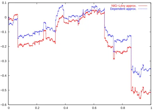
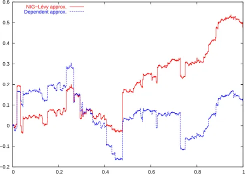
Simulation is done by first simulating a path for the approximation. For each jump in the compound Poisson, a dependent jump is generated from the condi-tional law of the copula. The second process is then constructed as in Equation (2.5). In Figures 2.3, 2.4 and 2.5 the former process is marked as ”NIG-Lévy approx”, while latter process is marked as ”Dependent approx”.
see the effect of copulas on high dependency. Clearly, with such high tail depen-dency in the lower (upper) tail there will also be reasonable high dependence in the upper (lower) tail as well using the Clayton copula.
−0.6 −0.5 −0.4 −0.3 −0.2 −0.1 0 0.1 0 0.2 0.4 0.6 0.8 1 NIG−Lévy approx. Dependent approx.
Figure 2.3: Gumbel withθ= 20, notice higher dependency in upper than lower
−0.2 −0.1 0 0.1 0.2 0.3 0.4 0.5 0.6 0 0.2 0.4 0.6 0.8 1 NIG−Lévy approx. Dependent approx.
Figure 2.4: Gumbel withθ= 10, notice higher dependency in upper than lower
tail. −1.5 −1 −0.5 0 0.5 1 1.5 0 0.2 0.4 0.6 0.8 1 NIG−Lévy approx. Dependent approx.
2.6.1
Implementation issues
There are some issues that should be assessed. First, using the same truncation on each of our dependent processes may not result in both marginal processes approximating the NIG-Lévy equally well. This stems from the direct effect
that different values of δ have on the error of the Brownian approximation.
Furthermore, choice has to be taken with regards to dependency in the large jumps. Since the dependence in the general case is not perfect, the copula may produce jumps that would lie inside(−, ), if one use the quantiles of the NIG-Lévy increments. Since the jumps are drawn from the truncated NIG-Lévy jump measure,ν, a jump in this inteval can be translated to either a negative jump
or a positive jump if the first jump is close to or −. This can change the
intensities somewhat, but not in a degree that will let the process be vastly different from a NIG-Lévy. This may not the behavior one expect the when introducing dependency in the jump sizes, but this is a direct consequence of the approximation. Approximation error of the dependent process may be slightly higher than the first due to the reasons mentioned above.
One alternative is to round this jump to the minimum size. This on the other hand breaks the dependency structure, while maintaining the Lévy measure of the processes. A second alternative is to fit e.g. a NIG-distribution to the random variates drawn from a jump measure and use the builtin quantile mech-anisms. However, this will as mentioned allow for values which are less than
. In either case, these implementation issues must be conquered on the cost
of flexibility. Working withν directly may give unexpected effects, but it does not break the dependency structure.
Another issue that should be noted is that of round-off errors in the algorithm. This can give very strange results, especially with the Frank copula, where one can have large variations due to round-off errors in the tails as the tails of the Lévy jump probability measure are rather light.1
Therefore, it is necessary to implement a sanity check since the algorithm seems sometimes to experience numerical instability. In certain cases, the quantile produced by the copula has been rounded to 1 or 0 for extreme events in the tails. This gives jumps that seem unreasonable. The numerical implementation is therefore critical. Small variation in the quantile numbers may in the tail produce large differences in actual jump size. This is often observed far out in the tail where the jump sizes are often determined in 4th or 5th significant digit.
2.6.2
Copula choice for financial applications
In simulation, large spread in some parts of the copula can give unexpected
results. For example, for the Clayton with θ = 2 Figure 2.1 shows that it
has low dependence in the upper tail, while still quite a bit in the lower tail. Because of the high spread in the upper tail, one can sometimes observe that the dependent processes that are generated experience some negative drift. This is
due to the way ν is defined, as with sufficient spread, a jump close to may
generate dependent jump of size − or less, or visa versa. One can have large
1
An initial jump of0
.38corresponds to0.9998quantile ,while the returned result from the
copula may be as low as0