Real-Time Medical Data Visualization
Rui Shen and Pierre Boulanger Department of Computing Science
University of Alberta
Edmonton, Alberta, Canada T6G 2E8
{rshen,pierreb}@cs.ualberta.ca
Abstract. Volumetric data rendering has become an important tool in various medical procedures as it allows the unbiased visualization of fine details of volumetric medical data (CT, MRI, fMRI). However, due to the large amount of computation involved, the rendering time increases dramatically as the size of the data set grows. This paper presents several acceleration techniques of volume rendering using general-purpose GPU. Some techniques enhance the rendering speed of software ray casting based on voxels’ opacity information, while the others improve tradi-tional hardware-accelerated object-order volume rendering. Remarkable speedups are observed using the proposed GPU-based algorithm from experiments on routine medical data sets.
1
Introduction
Volume rendering deals with how a 3D volume is rendered and projected onto the view plane to form a 2D image. It has been broadly used in medical applica-tions, such as for the planning of treatment [1] and diagnosis [2]. Unlike surface rendering, volume rendering bypasses the intermediate geometric representation and directly renders the volumetric data set based on scalar information such as density, and local gradient. This allows radiologists to visualize the fine details of medical data without prior processing such as the visualization of isosur-faces. Transfer functions are commonly employed for color mapping (including opacity mapping) to enhance the visual contrast between different materials. However, due to the large amount of computation involved, the rendering time increases dramatically as the size of the data set grows. Our objective is to pro-vide radiologists with more efficient volume rendering tools to understanding the data produced by medical imaging modalities, such as Computed Tomogra-phy (CT) and Magnetic Resonance Imaging (MRI). Hence, we introduce several techniques, including hardware implementation using commercial graphics pro-cessing unit (GPU), to enhance the rendering speed. This increased speed will allow radiologists to interactively analyze volumetric medical data in real-time and in stereo.
According to [3], volume rendering approaches can be classified into three main categories: object-order, image-order and domain methods. Some hybrid
G. Bebis et al. (Eds.): ISVC 2007, Part II, LNCS 4842, pp. 801–810, 2007. c
methods [4] [5] are proposed by researchers in recent years, but their funda-mental operations still fall into one of the three categories. The object-order approaches [6] [7] evaluate the final pixel values in a back-to-front or front-to-back fashion, i.e., the scalar values in each voxel are accumulated along the view direction. Such intuitive approaches are simple and fast, but often yield image artifacts due to the discrete selection of projected image pixel(s) [8]. This problem can be solved by using splatting [9], which distributes the contribu-tion of one voxel into a region of image pixels. While resampling in splatting is view-dependent, shear-warp [10] alleviates the complications of resampling for arbitrary perspective views. The input volume composed of image slices is trans-formed to a sheared object space, where the viewing rays are perpendicular to the slices. The sheared slices are then resampled and composited from front to back to form an intermediate image, which is then warped and resampled to get the final image. The image-order volume rendering [11] [12] is also in the category of ray casting or ray tracing. The basic idea is that rays are cast from each pixel on the final image into the volume and the pixel values are determined by com-positing the scalar values encountered along the rays with some predefined ray function. One typical optimization is early ray termination, which stops tracing a ray when the accumulated opacity along that ray reaches a user-defined thresh-old. Another common optimization is empty space skipping, which accelerates the traversal of empty voxels. Volume rendering can also be performed in the frequency domain using Fourier projection-slice theorem [13]. After the volume is transformed from the spatial domain to the frequency domain, a specific 2D slice is selected and transformed back to the spatial domain to generate the final image. All of the previous three categories of methods can be partially or en-tirely implemented in GPU for acceleration [14] [15] [16]. Hardware-accelerated texture mapping moves computationally intensive operations from the CPU to the GPU, which dramatically increases the rendering speed.
A detailed comparison between the four most popular volume rendering tech-niques, i.e., ray casting, splatting, shear-warp and 3D texture hardware-based methods, can be found in [17]. Experimental results demonstrate that ray casting and splatting generate the highest quality images at the cost of rendering speed, whereas shear-warp and 3D texture mapping hardware are able to maintain an interactive frame rate at the expense of image quality. When using splatting for volume rendering, it is difficult to determine parameters such as the type and radius of kernel, and the resolution of the footprint table to achieve an optimal appearance of the final image [8]. In shear-warp, the memory cost is high since three copies of the volume need to be maintained. The frequency domain meth-ods perform fast rendering, but is limited to orthographic projections and X-ray type rendering [13].
2
Software-Based Accelerated Ray Casting
Software-based ray casting produces high-quality images, but due to the huge amount of calculation, the basic algorithm suffers from poor real-time
performance. To accelerate software ray casting, there are two common accel-eration techniques as mentioned in the previous section: empty space skipping and early ray termination.
Empty space skipping is achieved via the use of a precomputed min-max oc-tree structure. It can only be performed efficiently when classification is done before interpolation,i.e.,when the scalar values in the volume are converted to colors before the volume is resampled. This often produces coarser results than applying interpolation first. If empty space skipping is applied with interpola-tion prior to classificainterpola-tion, one addiinterpola-tional table lookup is needed to determine whether there are non-empty voxels in the current region. Nevertheless, the ma-jor drawback with such kind of empty space skipping lies in that every time the transfer functions change, the data structure that encodes the empty regions or the lookup table needs to be updated.
Early ray termination exploits the fact that when a region becomes fully opaque or is of high opacity, the space behind it can not be seen. Therefore, ray tracing stops at the first sample point where the cumulative opacity is larger than a pre-defined threshold. The rendering speed is often far from satisfactory, even for medium-size data sets (e.g.,2563). In order to accelerate the speed, one can use acceleration techniques such as β-acceleration [18]. The fundamental idea of theβ-acceleration is that as the pixel opacity (theβ-distance) along a ray accumulates from front to back, less light travels back to the eye, therefore, fewer ray samples need to be taken without significant change to the final image quality. In other words, the sample interval along each ray becomes larger as the pixel opacity accumulates. Unlike β-acceleration, which depends on a pyrami-dal organization of volumetric data, here the jittered sample interval is applied directly to the data set. This reduces the computational cost of maintaining an extra data structure, especially when the transfer function changes. Instead of going up one level in the pyramid whenever the remaining pixel opacity is less than a user-defined threshold after a new sample is taken, the sample interval is modified according to a function of the accumulated pixel opacity:
s=s×(1.0 +α×f) (1) where s denotes the length of the sample interval;α denotes the accumulated opacity; and f is a predefined jittering factor. The initial value of s is set by the user. Normally, the smaller s the better image quality. For every sample point, the remaining opacityγis compared against a user-specified threshold. If
γis less than the threshold, the current sample interval is adjusted according to Equation 1. We term this acceleration technique asβ-acceleration.
To further enhance the performance of software ray casting during interaction, the sample interval is automatically enlarged to maintain a high rendering speed, and once interaction stops, the sample interval is set back to normal. When multiple processors are available, the viewport is divided into several regions and each processor handles one region.
The whole process is executed in the CPU and main memory. The enhanced algorithm is illustrated in the following pseudo-code. Not only is this software
approach suitable for computers with low-end graphics cards, but since parallel ray tracing is used, it is also suitable for multi-processor computers or clusters. Accelerated Software-Based Ray Casting
Break current viewport into N regions of equal size
Initialize early ray termination threshold Γ
Initialize jittering start threshold Γ
Initialize jittering factor f
Initialize sample interval s
For each region
For every pixel in the current region
Compute ray entry point, direction, maximum tracing distanceD
While the traced distance d < D and γ < Γ
Interpolate at current sample point
Get opacity value α according to opacity mapping function
If α= 0
Compute pixel color according to color mapping function
γ=γ×(1.0−α) End If If γ < Γ s=s×(1.0 +α×f) End If d=d+s
Compute next sample position End While
End For End For
3
GPU-Based Object-Order Volume Rendering
based object-order volume rendering has several advantages over GPU-based image-order volume rendering. First, perspective projections can be more easily implemented in object order, since only a proper scaling factor needs to be assigned to each slice based on several viewing parameters. In ray casting, the direction of each ray needs to be determined individually. Second, as pointed out in [19], GPU-based ray casting has the limitation that it can only render volumes that fit in texture memory. Since ray tracing needs to randomly access the whole volume, it is impossible to break the volume into sub-volumes and load each sub-volume only once per frame. Finally, most of the speedup from GPU-based ray casting comes from empty space skipping, and ray casting with only early ray termination shows close performance to object-order volume rendering while both implemented in the GPU, as compared in [15].
Other implementations generate the proxy polygons that textures are mapped to in the CPU, and use the fragment shader for trilinear interpolation and tex-ture mapping. Little work has been done to exploit the vertex shader in the
Fig. 1.The five intersection cases between a proxy plane and the volume bounding box, and the traversal order of the bounding box edges
hardware-accelerated volume rendering pipeline. Our accelerated rendering algo-rithm is based on the algoalgo-rithm proposed by Rezk-Salama and Kolb [20], which balances the workload between the vertex shader and the fragment shader. Based on the observation of different box-plane intersection cases, the generation of proxy polygons can be moved from the CPU to the GPU. The intersection be-tween a proxy plane and the bounding box of the volume may have five different cases, ranging from three intersection points to six, as illustrated in Figure 1. Letn·(x, y, z) =drepresent a plane, wherenis the normalized plane normal anddis the signed distance between the origin and the plane, and letVi+λei,j
represent the edge Ei,j from vertex Vi to Vj, where eij = Vj −Vi, then the
intersection between the plane and the edge can be computed by
λi,j=
d−n·Vi
n·ei,j ,n·ei,j= 0;
−1, otherwise. (2)
Ifλi,j∈[0,1], then it is a valid intersection; otherwise, there is no intersection.
The edges of the volume bounding box are checked following a specific or-der, so that the intersection points can be obtained as a sequence that forms a valid polygon. IfV0 is the front vertex (the one closest to the viewpoint) and
V7 is the back vertex (the one farthest from the viewpoint), then the edges are
divided into six groups, as shown in Figure 1 marked with different gray levels and line styles. For a given planeP lparallel to the viewport that does intersect with the bounding box, there is exactly one intersection point for each of the three groups (solid lines), and at most one intersection point for each of the other
three groups (dotted lines). The six intersection pointsP0 to P5 are computed
as described in Table 1. For the other seven pairs of front and back vertices, the only extra computation is to map each vertex to the corresponding vertex in this case, which can be implemented as a simple lookup table.
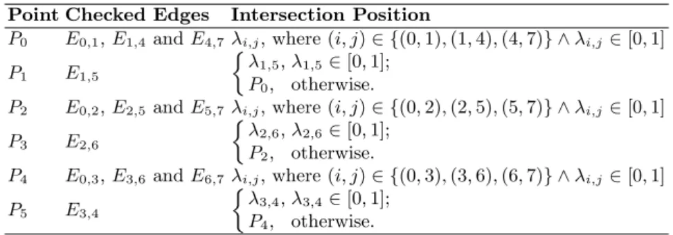
Table 1.The computation of the intersection points
Point Checked Edges Intersection Position
P0 E0,1,E1,4 andE4,7 λi,j, where (i, j)∈ {(0,1),(1,4),(4,7)} ∧λi,j∈[0,1]
P1 E1,5
λ1,5, λ1,5∈[0,1];
P0, otherwise.
P2 E0,2,E2,5 andE5,7 λi,j, where (i, j)∈ {(0,2),(2,5),(5,7)} ∧λi,j∈[0,1]
P3 E2,6
λ2,6, λ2,6∈[0,1];
P2, otherwise.
P4 E0,3,E3,6 andE6,7 λi,j, where (i, j)∈ {(0,3),(3,6),(6,7)} ∧λi,j∈[0,1]
P5 E3,4 λ3,4, λ3,4∈[0,1];
P4, otherwise.
In Rezk-Salama and Kolb’s method, the coordinates of a sample point in the world coordinate system are required to be the same as the coordinates of the corresponding sample point in the texture coordinate system. However, this is not true for most cases, where the sizes of one volume are different in the two coordinate systems. The box-plane intersection test is carried out in the data coordinate system. Since typically the texture coordinates need to be normalized to the range between [0,1], a conversion of valid intersection points’ coordinates is required. If the point Pk intersects the edge Ei,j at position λi,j, then each
coordinate of the resulting texture-space intersection pointPk is obtained by
Pk.p= ⎧ ⎨ ⎩ Vi.p−min(Bp) max(Bp) ,ei,j.p= 0; λi,j, ei,j.p >0; 1−λi,j, ei,j.p <0. (3)
wherepdenotes eitherx,y or z andB denotes the volume bounding box. The coordinates of Pk are then scaled and translated in order to sample near the center of the cubic region formed by eight adjacent voxels in texture memory.
To further accelerate the rendering process, we also propose another enhance-ment that the sample interval is adjusted based on the size of the volume in the world coordinate system and the distance from the viewpoint to the volume. This idea of adaptive sample interval is similar to the concept of level-of-detail (LOD) in mesh simplification. The sample interval is calculated by:
s=S×F
max(d)
max(Bx,By ,Bz) (4)
where S denotes the constant initial sample interval; F 1 denotes the pre-defined interval scale factor;Bx, By and Bz denote the length of the volume
bounding boxB in the x, y, andz-direction respectively; and max(d) denotes the distance between the farthest vertex ofB and the view plane.
Now that the proxy polygons are generated, one can then perform texture mapping. The fragment shader performs two texture lookups per fragment to attach textures onto the proxy polygons. The first texture lookup gets the scalar value associated with the sample point from a 3D texture that holds the vol-umetric data. The hardware does the trilinear interpolation automatically for every sample. The second texture lookup uses the scalar value to get the cor-responding color from a 2D texture that encodes the transfer function. Then, the textured polygons are written into the frame buffer from back to front to produce the final image.
The vertex program and the fragment program are both written in Cg, a high-level shading language developed by NVIDIA. To exploit the most power-ful profile supported by a graphics card, the shader programs are compiled at runtime instead of at compile time. To accommodate graphics cards with dif-ferent vertex processing capabilities, the amount of work assigned to the vertex shader should vary from card to card as graphic cards do not have all the same processing capabilities. The more capable the programmable graphics hardware is, the larger the amount of processing load is moved from the CPU to the vertex shader. Currently, our vertex program has variations for all the OpenGL ver-tex program profiles supported by the Cg compiler. The fragment program only requires basic Cg profiles to compile. Therefore, theoretically the proposed GPU-based volume rendering program can be executed on most commodity computers with a good-quality programmable graphics card.
4
Results
The algorithms were tested on a dual-core 2.0GHz computer running Windows XP with a 256MB-memory NVIDIA GeForce 7800 GTX graphics card. The data used for testing is a medium-size (512x512x181) CT-scan of the pelvic region.
Software-based ray casting provides high quality images, but only with small viewports or for small data sets it can maintain an acceptable rendering speed, even with the proposedβ-acceleration. The rendering times using software ray casting with both early ray termination andβ-acceleration and with only early ray termination are enumerated in the first two columns of Table 2. Figure 2(a) depicts the two cases’ performance curves with respect to the viewport size. The x-axis is the size of the viewport in pixels and the y-axis is the rendering time in seconds. The dark gray line denotes the performance of the method without
β-acceleration, and the other line denotes the performance of the one withβ -acceleration. On average, software ray casting with both early ray termination (Γ=0.02) andβ-acceleration (Γ=0.6 andf=0.1) takes 28% less time than that with only early ray termination (Γ=0.02). The resulting images are shown in Figure 3(a)(b). There is no noticeable difference between these two images.
High-quality images and interactive rendering speed are both achieved by exploiting the processing power of the GPU. The rendering times under four
Table 2.The rendering times using different acceleration techniques Viewport Size Rendering Time (unit: second)
(unit: pixel) WithoutβWithβTex’ 1.0 Tex’ 1.15 Tex 1.0 Tex 1.15 200x200 0.172 0.125 0.031 0.016 0.015 0.015 300x300 0.422 0.281 0.031 0.016 0.015 0.015 400x400 0.688 0.484 0.031 0.016 0.015 0.015 500x500 1.078 0.750 0.047 0.031 0.031 0.015 600x600 1.641 1.125 0.047 0.031 0.031 0.016 700x700 2.078 1.562 0.062 0.047 0.047 0.031 800x800 2.704 2.187 0.062 0.047 0.047 0.031 900x900 3.391 2.469 0.078 0.062 0.062 0.047 1000x1000 4.312 3.062 0.094 0.078 0.078 0.047 0 0.5 1 1.5 2 2.5 3 3.5 4 4.5 5 200x200 300x300 400x400 500x500 600x600 700x700 800x800 900x900 1000x1000
Viewport Size (unit: pixel)
Rendering Time (unit: second)
Without Beta'-Acceleration With Beta'-Acceleration
(a) Ray Casting.
0 0.01 0.02 0.03 0.04 0.05 0.06 0.07 0.08 0.09 0.1 200x200 300x300 400x400 500x500 600x600 700x700 800x800 900x900 1000x1000
Viewport Size (unit: pixel)
Rendering Time (unit: second)
Tex 1.0 Tex 1.15 Tex' 1.0 Tex' 1.15
(b) Object-Order.
Fig. 2.The comparison of the rendering times using different acceleration techniques
different conditions are enumerated in Table 2.Tex’ 1.0 denotes no acceleration; Tex’ 1.15 denotes adaptive sample interval with interval scale factorF=1.15; Tex 1.0 denotes only with vertex shader acceleration; Tex 1.15 denotes with both acceleration techniques and F=1.15. Figure 2(b) gives a comparison of the performance curves under the four different conditions. In all cases, the rendering time increases as the viewport grows, but even for the 1000x1000 viewport the rendering times are below 0.1 second,i.e.,the rendering speeds are above the psycho-physical limit of 10 Hz. With only adaptive sample interval enabled, whenF=1.15, we get an average 33% speedup. With only vertex shader acceleration enabled, the algorithm’s performance is almost the same as Tex’ 1.15. With both acceleration techniques enabled, whenF=1.15, an average 53% speedup is achieved with respect to the Tex’ 1.0 case and an average 28% speedup is achieved with respect to the Tex’ 1.15 case. The final images are shown in Figure 3(c)-(f), together with the images produced by software ray casting. From these images, no significant difference can be observed between the image quality of image-order methods and that of object-order methods, as long as the original data set is at high resolution.
(a) Withoutβ. (b) Withβ. (c) Tex’F = 1.0.
(d) Tex’F = 1.15. (e) TexF = 1.0. (f) TexF= 1.15. Fig. 3.Volume rendering results of a CT-scanned pelvic region
5
Conclusion
In this paper, we have presented several volume rendering acceleration techniques for medical data visualization.β-acceleration enhances the rendering speed of software-based ray casting using voxels’ opacity information, while vertex shader proxy polygon generation and adaptive sample interval improve the performance of traditional hardware-accelerated object-order volume rendering. Remarkable speedups are observed from experiments on average-size medical data sets. We are now working on incorporating theβ-acceleration into the GPU ray casting pipeline, which may be more efficient than our current GPU-based object-order method. Moreover,we are also exploring more efficient and effective rendering algorithms using GPU clusters to handle larger and larger data sets produced by doppler MRI and temporal CT.
References
1. Levoy, M., Fuchs, H., Pizer, S.M., Rosenman, J., Chaney, E.L., Sherouse, G.W., Interrante, V., Kiel, J.: Volume rendering in radiation treatment planning. In: Proceedings of the first conference on Visualization in biomedical computing, pp. 22–25 (1990)
2. Hata, N., Wada, T., Chiba, T., Tsutsumi, Y., Okada, Y., Dohi, T.: Three-dimensional volume rendering of fetal MR images for the diagnosis of congenital cystic adenomatoid malformation. Academic Radiology 10, 309–312 (2003) 3. Kaufman, A.E.: Volume visualization. ACM Computing Surveys 28, 165–167
4. Hadwiger, M., Berger, C., Hauser, H.: High-quality two-level volume rendering of segmented data sets on consumer graphics hardwarem. In: VIS 2003: Proceedings of the conference on Visualization 2003, pp. 301–308 (2003)
5. Mora, B., Jessel, J.P., Caubet, R.: A new object-order ray-casting algorithm. In: VIS 2002: Proceedings of the conference on Visualization 2002, pp. 203–210 (2002) 6. Drebin, R.A., Carpenter, L., Hanrahan, P.: Volume rendering. In: SIGGRAPH 1988: Proceedings of the 15th annual conference on Computer graphics and inter-active techniques, pp. 65–74 (1988)
7. Upson, C., Keeler, M.: V-buffer: visible volume rendering. In: SIGGRAPH 1988: Proceedings of the 15th annual conference on Computer graphics and interactive techniques, pp. 59–64 (1988)
8. Shroeder, W., Martin, K., Lorensen, B.: The visualization toolkit: an object-oriented approach to 3D graphics, 4th edn. Pearson Education, Inc. (2006) 9. Mueller, K., Shareef, N., Huang, J., Crawfis, R.: High-quality splatting on
rectilin-ear grids with efficient culling of occluded voxels. IEEE Transactions on Visualiza-tion and Computer Graphics 5, 116–134 (1999)
10. Lacroute, P., Levoy, M.: Fast volume rendering using a shear-warp factorization of the viewing transformation. In: SIGGRAPH 1994: Proceedings of the 21st annual conference on Computer graphics and interactive techniques, pp. 451–458 (1994) 11. Levoy, M.: Efficient ray tracing of volume data. ACM Transactions on Graphics 9,
245–261 (1990)
12. Yagel, R., Cohen, D., Kaufman, A.: Discrete ray tracing. IEEE Computer Graphics and Applications 12, 19–28 (1992)
13. Entezari, A., Scoggins, R., M¨oller, T., Machiraju, R.: Shading for fourier volume rendering. In: VVS 2002: Proceedings of the 2002 IEEE symposium on Volume visualization and graphics, pp. 131–138 (2002)
14. Van Gelder, A., Kim, K.: Direct volume rendering with shading via three-dimensional textures. In: VVS 1996: Proceedings of the, symposium on Volume visualization (1996) pp. 23–30 (1996)
15. Kruger, J., Westermann, R.: Acceleration techniques for GPU-based volume ren-dering. In: VIS 2003: Proceedings of the 14th IEEE Visualization 2003, pp. 287–292 (2003)
16. Viola, I., Kanitsar, A., Gr¨oller, M.E.: GPU-based frequency domain volume ren-dering. In: SCCG 2004: Proceedings of the 20th spring conference on Computer graphics, pp. 55–64 (2004)
17. Meißner, M., Huang, J., Bartz, D., Mueller, K., Crawfis, R.: A practical evaluation of popular volume rendering algorithms. In: VVS 2000: Proceedings of the 2000 IEEE symposium on Volume visualization, pp. 81–90 (2000)
18. Danskin, J., Hanrahan, P.: Fast algorithms for volume ray tracing. In: VVS 1992: Proceedings of the 1992 workshop on Volume visualization, pp. 91–98 (1992) 19. Scharsach, H.: Advanced GPU raycasting. In: Proceedings of CESCG 2005, pp.
69–76 (2005)
20. Rezk-Salama, C., Kolb, A.: A vertex program for efficient box-plane intersection. In: Proceedings of the 10th international fall workshop on Vision, modeling and visualization (2005)