OSG Based Real time Volume Rendering Algorithm for Electromagnetic Environment

2018 International Conference on Computer Science and Software Engineering (CSSE 2018) ISBN: 978-1-60595-555-1

OSG Based Real-time Volume Rendering

Algorithm for Electromagnetic Environment

Beibei Han

1

ABSTRACT

The electromagnetic environment is widespread and very complex. Due to the invisibility of the electromagnetic environment, the direct volume rendering technique can be used to show the complex electromagnetic environment. In this paper, the Irregular Terrain Model (ITM) electromagnetic wave propagation model and the coordinate transformation are used to simulate the electromagnetic environment. In the three-dimensional digital GlobelGIS platform, the improved ray casting algorithm is applied to render the electromagnetic field and design the transfer function which is used to express different electromagnetic power intensity with different colors and opacities. Considering the problem that the traditional ray casting algorithm, which uses the OpenGL graphical interface, cannot be integrated into the GlobelGIS platform directly, so the ray casting algorithm that based on OSG and the GLSL shading language for hardware-acceleration are proposed. The simulation results show that this method can render multi-source electromagnetic environment on the GlobelGIS platform in real-time and interactively. The volume rendering algorithm is not only suitable for the rendering of electromagnetic, but also for the visualization of volume data in other applications.

Beibei Han

INTRODUCTION

Due to the invisibility of the electromagnetic environment, the complex electromagnetic environment needs to be displayed on three-dimensional digital platform through visualization, which has great significance for helping the user to understand the situation of the electromagnetic environment intuitively.

One of the best approaches to visualize the electromagnetic environment is the volume rendering1. Volume rendering maps the three-dimensional image to the two-dimensional image on screen directly. Volume rendering can display internal details of volume data and provide support for users to observe and understand spatial data. Ray casting algorithm 2 is one of the typical volume rendering algorithm which is proposed many years ago; however, it is still very popular since it has a good rendering effect. But the calculation of ray casting is complicated. With the development of GPU, the GPU general-purpose computing technology is applied to the ray casting to accelerate the algorithm in some extent 3. Researchers continue to investigate and improve the GPU-based ray casting algorithm [4,5,6] , which makes it widely used.

The [7] uses the OpenGL graphical interface and GLSL shading language to implement the ray casting algorithm to visualize the electromagnetic field; however, the authors do not apply the visualization results to a specific platform. Similar to [7], the [8] uses the same graphical interface and shading language to visualize the electromagnetic environment with ray casting algorithm on a three-dimensional digital globe platform. The [9] achieves the parallel ray casting algorithm based on CUDA architecture and the results are attached to osgEarth simply. GlobelGIS 3D Digital Earth is a platform which is developed based on the Qt and OSG 3D rendering engine; moreover, it has cross-platform features. However, the traditional GPU-based ray casting algorithm is based on the OpenGL [10] graphical interface and cannot be integrated into the GlobelGIS platform directly. In order to solve this problem, based on the in-depth study of the principle of OSG architecture and ray casting algorithm, this paper uses OSG [11] 3D rendering engine interface and GLSL language to implement the hardware-accelerated ray casting volume rendering algorithm, which is integrated on the GlobelGIS platform. Through coordinate transformations, the complex electromagnetic environment modeling that based on ITM model and electromagnetic rendering are realized on this platform to meet the users' real-time interactive control. Ray casting algorithm that based on OSG and GLSL shading language is also suitable for volume rendering in other scenes.

ITM BASED ELECTROMAGNETIC ENVIRONMENT CALCULATION MODEL

the propagation distance gradually. The Irregular Terrain Model (ITM)[12,13,14] developed by Longley and Rice and is used for predicting propagation attenuation of electromagnetic waves in space. Based on the ITM model, the attenuation value of the energy of each electromagnetic equipment in three-dimensional space is calculated; moreover, the power values of the various points in the three-dimensional space also can be calculated according to the transmitting power of the equipment, which can be used to design a complex electromagnetic environment calculation model.

ITM Based Electromagnetic Environment Model Design

ITM irregular terrain model is suitable for the equipment which the antenna height is between 0.5m to 3000.0m, the frequency is between 20MHz to 20GHz, and the propagation distance is less than 2000km. The ITM model is divided into Point-To-Point Model and Area Prediction Model based on the detailed degree of terrain data. Due to the Point-To-Point Model can accurately consider the impact of irregular terrain on electromagnetic wave propagation, so this paper designs the electromagnetic environment model based on the Point-To-Point Model.

The electromagnetic propagation attenuation value Aref is a piecewise function on the propagation distance d and can be calculated as follows:

(

)

(

)

In these three piecewise functions, d<dls means the line-of-sight region, dls<d<dx means the diffraction region, and dx<d means the scattering region. The parameters Ael, K1, K2, Aed, md, Aes, ms, dls and dx are calculated based on electromagnetic theory and statistical methods, which is given in [15].

The wave propagation path loss of electromagnetic in free space is calculated as: R lg f lg .

L_fs =3245+20 +20

(2)

In Equation (2), f is the frequency of electromagnetic waves which the unit is MHz; R is the electromagnetic wave propagation distance and the unit is km. The total propagation loss of electromagnetic waves is:

ref fs A

L

Loss = + (3)

Based on the antenna gain and the transmit power of the device, the electromagnetic power intensity value at any point of the three-dimensional space can be calculated:

where Pr is the received power intensity value at a certain point of the three-dimensional space; Pt is the transmitted power intensity value of the device in dBW; G is the antenna gain in dB; Loss is the total electromagnetic wave propagation loss calculated in Equation (3) in dB; Ls is the system loss and other losses, etc., generally 3-5dB [16].

Spatial Area Discretization Sampling

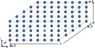
Because the electromagnetic field is full of the space, it is a three-dimensionally continuous data field. To visualize the electromagnetic field, it should be discretizedfirstly and render next. Taking into account the convenience of calculation, storage and visualization, the electromagnetic field is discretized into the regular grid data with a certain interval; moreover, the uniform sampling is made in the three coordinate axes of the local Cartesian coordinate system and form the three-dimensional scalar field of the electromagnetic field of regular grid. With this method, the size of the three-dimensional scalar data of the electromagnetic field is m k n× × , which is shown in Figure 1.

Terrain Extraction Based on ITM Model

When calculating the propagation path loss from the radiation source to the receiving point based on Point-to-Point Prediction Mode (ITM), the terrain elevation information between these two points needs to be provided. In this paper, regular grid DEM [17,18] is used to extract the elevation data between these two points. If the sampling point is not on the regular grid intersection, the bilinear interpolation method should be used to calculate the elevation value of this point, as shown in Figure2(a). In order to ensure the accuracy of the calculation, the sampling interval should be less than the resolution of the DEM when extracting the terrain elevation data on the propagation path. After extracting the elevation data on the propagation path, the electromagnetic power of the receiving point can be obtained from the model designed in 1.1 by combining the heights of the radiation source h1 and the receiving point h2. This is shown in Figure2(b).

(a)DEM regular grid (b) Terrain samplingCross Section

Figure 2.Terrain extraction diagram.

Coordinate Transformation

In this paper, the electromagnetic environment volume data is organized in a local three-dimensional Cartesian coordinate system. The center of the sampling range is regarded as the origin of the local coordinate system. The Xlocal axis coincides with the long axis of the earth ellipsoid, i.e., the east direction; Ylocal coincides with the minor axis of the ellipsoid, that is, the direction is north; the

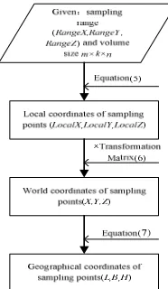
Zlocal axis coincides with the normal of the ellipsoid, that is, vertically upward. The sketch map is shown in Figure 3. Given the geographic coordinates of the origin point OLocal of the local coordinate system, a transformation matrix from local coordinates to world coordinates can be obtained by (6). Using the method introduced in Figure 4, we can calculate the geographic coordinates of each sampling point. Knowing the geographic coordinates of the radiation source and each sampling point, we can calculate the distance between these two points; then the method introduced in Section 1.3 is used to sample the terrain at regular intervals between these two points. Finally, the model in Section 1.1 is applied to calculate the electromagnetic power intensityof m k n× × sampling points.

Figure 3.Coordinate System. Figure 4.Sampling point coordinate

2 1

2 1

1

R a ng eX R a ng eX

L o calX i

m R a ng eY R a ng eY

L o calY j

k R a ng eZ

L o calZ h

n  = − + ∗  ₋   = − + ∗  −   = ∗  −

 ₍₅₎

In (5), RangeX and RangeY are 450km,

1 3 2 1

0 −

= ,, , m

i _, j=0 1 2 3, , , k−1,h=0 1 2 3, , , n−1_{. The local coordinates of each} sampling point can be calculated by (5).

( ) ( )

( ) ( ) ( ) ( ) ( ) ( ) ( ) ( ) ( ) ( )

0 0

0 0 0 0 0

0 0 0 0 0

0

sin L cos L

cos L sin B sin L sin B cos B

cos L cos B sin L cos B sin B

−     − ∗ − ∗     ∗ ∗

  (6)

where L0 represents the longitude of the origin point OLocal and B0 represents the

latitude of the origin point OLocal.

           − + =         ∗ ∗ − + ∗ ∗ + =       = N B cos Y X H cos a e Y X sin b e Z arctan B X Y arctan L ' 2 2 3 2 2 2 3 2 θ θ (7) where, 2 2 2 2 b b a e' = −

, e sin B a N

2

2 1− ∗ = ,       ∗ + ∗ = b Y X a Z arctan 2 2 θ , 2 2 2 2 a b a e = −

;

(X,Y,Z)

ELECTROMAGNETIC ENVIRONMENT VOLUME RENDERING

The GlobelGIS platform is the 3D digital earth that developed based on Qt and OSG [19] 3D rendering engine. The traditional hardware-accelerated ray casting algorithm is usually based on the OpenGL graphical interface and cannot be integrated into the platform directly. After deeply studying OSG architecture and ray casting algorithm, this paper improves the traditional ray casting algorithm and implements it by using 3D rendering engine OSG and GLSL shading language. Finally, the improved algorithm is integrated into GlobelGIS platform to visualize the electromagnetic environment.

OSG Based Ray Casting Algorithm

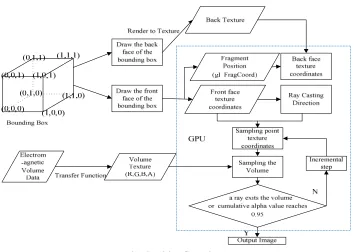
The OSG 3D rendering engine consists by a series of graphics-related functional modules, it provides scene management and graphics rendering optimizations primarily for the development of graphical image applications [20]. Because of its cross-platform nature, it can be run on most types of operating systems, which allows the OSG developers to develop on their favorite platforms and configure them based on the platform users’ demand. Compared with the industry standard OpenGL, OSG encapsulates and provides a multitude of algorithms to enhance the program performance in addition to open-source and cross-platform features. Therefore, this paper uses the OSG and GLSL shading language to achieve the hardware-accelerated ray casting algorithm, the algorithm implementation process is shown in Figure 5.

(b) algorithm flow chart

Figure 5. Ray casting algorithm.

The algorithm is shown as follows: (1)Back face generation

Creating a CVolumeRenderGeometry object BackFaceGeometry, setting the rendering properties through the node's rendering state set StateSet, and removing the front faces of the bounding box by setting the rendering mode to

osg::CullFace::FRONT to get the back faces of the bounding box. By

FBO(Frame Buffer Object) and rendering the result back to the texture BackFace, the exiting position of the ray can be got. Among them, the coordinates of the vertices of the bounding box are equal to the color of the vertex and the coordinates of the texture.

Note that when using the OSG interface to render back to texture BackFace, first, the camera's RenderTargetImplementation needs to be set. However, it is not possible to set the setRenderTargetImplementation of the scene's main camera directly to FRAME_BUFFER_OBJECT, since the scene will not be visible. Because the main camera corresponds to the rendering stage has been bound the scene drawn results to the FBO. The correct approach is to add a CameraNode in the scene tree and set the RenderTargetImplementation to FBO mode, then set its render order to PRE_RENDER render preferentially, which ensure that the camera executes rendering before the main scene [21]. This paper adds a

content (mainly COLOR_BUFFER) to the texture BackFace instead of rendering it in a viewport.

(2)The direction of ray

Creating a CVolumeRenderGeometry Object FrontFaceGeometry and drawing the bounding box again, removing the back faces of the bounding box via

osg::CullFace::BACK, which gives the starting point of the bounding box .

Instead of rendering the front faces of the bounding box to texture, the fragment program is launched directly in this time. The back face coordinates , minus the front face coordinates yield ray direction vectors(RayDir) and lengths. The multi-step ray casting algorithm in [3] needs to draw the bounding box multiple times and starts the fragment program several times to determine the exit positions and direction of ray.

(3)Ray Casting

Ray casting process in the fragment program with a for loop, the ray from the starting point, each step forward to get a resampling point R(n), with the sampling location of the three-dimensional coordinates to find the three-dimensional texture VolumeTex, you can get the resampling point color and opacity

colorSample, as shown in Equation (9).

colorSample = texture3D(VolumeTex,R(n)) (9)

(4)Front-to-Back Compositing

Before the volume texture is loaded into the memory, different values of the volume data are given different color and opacity based on the value of electromagnetic power and the transfer function that designed in Section 2.2. Therefore, according to find the 3D volume texture, the value of colorSample can be obtained. The color and opacity of the sampling points on the ray can be accumulated according to the ray absorption and emission model [22] from front to back. Repeating step (3) until the ray leaving bounding box or the opacity accumulation is greater than 0.95. Among them, the opacity accumulation is greater than 0.95, which can accelerate the algorithm to some extent.

Transfer Function Design

In ray casting algorithm, the transfer function maps the data properties to certain optical properties (such as color and opacity). The design of the transfer function determines the quality of the resulting image [23].

For the three-dimensional scalar electromagnetic field used in this paper, the data attribute is the power of the sampling point in space. In this paper, the linear piecewise function is used to map the power values to different colors and opacities to distinguish the magnitude of the power of the electromagnetic field.

ending points of each section. Taking the red component R as an example, the color of the starting point and the ending point are represented by Rstart and Rend, respectively; the corresponding of the color Rvalue to the field data Value that distributed in the segment [Vstart,Vend]can be calculated by Equation (10) . The corresponding G, B, and A can be calculated in the same way. The volume texture's internal texture format and pixel format are set to GL_RGBA. Before the 3D texture is loaded into the memory, the electromagnetic field volume data have been classified and can be directly drawn.

( end start) start

end end start

value R R

V V

V Value R

R × −

− − +

=

(10)

Vstart and Vend represent the start and end electromagnetic field values of a section

respectively, Rstart and Rend represent the start and end red component values of the

section respectively . Value is an electromagnetic power value in the section [Vstart,Vend], Rvalue represents the magnitude of the red component corresponding to the Value.

EXPERIMENTAL RESULTS

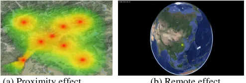
The experiment is implemented in Win7-64 bit operating system. Computer hardware configuration is: Inter (R) Core i7-6700HQ CPU 8GB, NVIDIA GeForce GTX1060. Software Environment: Qt4.8.6, Microsoft Visual 2010 compiler, OSG3.2.0. Eight electromagnetic devices are set in the GlobelGIS platform; the devices are equipped with omni-directional antenna, horizontal polarization. ITM radio propagation model parameters are set as: Surface Refractivity 301N-units, Dielectric Constant of Ground 15F / m, Conductivity of Ground 0.005S / m. DEM data resolution is 90.0 meters, terrain sampling interval is set to 76.5 meters. Using the improved ray casting algorithm, the electromagnetic environment data field is rendering on GlobelGIS platform. Figure 6 illustrates the effect of the electromagnetic environment data field on the platform in short distance and long distance, respectively. When the size of electromagnetic field data is 64 × 64 × 32, the coverage area is 450km × 450km and the window size is 1920 × 1080 pixels. The average frame rate reachs the max frame rate setting of 60 frames per second (set the maximum frame rate is 60 frames per second). In [8] ,the average frame rate is 12 frames per second when the window size is 1024 × 768. In [24] , the average frame rate is 40 frames per second when the

(a) Proximity effect (b) Remote effect

window size is 880 × 760 and rendering results are not integrated on a certain platform. Compared with [8] and [24], in this paper, the ray casting algorithm based on OSG satisfies the requirements of real-time interactive control and provides the time support for other operations. And the rendering results are integrated on GlobelGIS platform.

CONCLUSION

Since the traditional ray casting algorithm uses OpenGL graphical interface and cannot be integrated into the GlobelGIS platform directly, a ray casting algorithm that based on OSG and GLSL shading language for accelerating the hardware is proposed in this paper. Because we use the local three-dimensional Cartesian coordinate system to organize the volume data, so it is necessary to transform the coordinate system between the local coordinate system, the world coordinate system and the geographic coordinate system before calculating the electromagnetic environment volume data. When using the ITM model to calculate the electromagnetic environment volume date, the influence of the terrain and the atmosphere are taken into account. Finally, the real-time rendering of electromagnetic volume data is implemented on GlobelGIS platform. The results show that even the volume data is generated based on the ITM model, the improved ray casting volume rendering algorithm is also suitable for the visualization of volume data in other applications.

ACKNOWLEDGMENTS

This work was financially supported by National Key R&D Plan (2016YFB0502300) fund.

REFERENCES

1. Wu Yingnian, Zhang Lin, Zhang Lifang, et al. Survey on Electromagnetic Environment Simulation and Visualization [J].Journal of System Simulation, 2009, 21(20):6332-6338. 2. Marc Levoy . Display of Surfaces from Volume Data. IEEE Computer Graphics and

Applications1988, 8(3): 29-37.

3. Kruger J, Westermann R. Acceleration techniques for GPU-based volume rendering. Proceedings of IEEE Conference onVisualization. 2003, 287-292.

4. Zhang Aguan, Jiang Huiqin, Ma Ling,et al. An improved ray casting algorithm based on GPU[J].Computer Engineering & Science, 2017, 39(01):145-150.

5. Liang Chengzhi, Gao Xinbo, Zou Hua,et al. Accelerated GPU Ray-casting Algorithm Based on Space Leaping [J]. Journal of Image and Graphics, 2009, 14(8):1685-1688. 6. Yang Jinzhu, Zhao Dazhe, Li Wei,et al. The Research Volume Rendering Algorithm Based

on GPU[J]. Acta Electronica Sinica,2010,38(2A):202-206.

Situation with Graphics Processing Unit Based on Ray-casting Algorithm [J].Acta Armamentarii, 2015, 36(12):2306-2314.

8. Yang Chao,Xu Jiangbin,Wu Lingda.Hardware Accelerated Volume Visualization in Virtual Electromagnetic Environment [J].Journal of Beijing University of Posts and Telecommunications, 2011, 34(01):55-59.

9. Feng Xiaomeng, Wu Lingda, Dong Shiwei. CUDA Accelerated Real-time Rendering for Dynamic Electromagnetic Environment Volume Data [J]. Journal of System Simulation, 2014, 26(09):2044-2049.

10. Dave Shreiner, The Khronos OpenGL ARB Working Group. OpenGL Programming Guide(Version 7). Li Jun,Xu Bo, et al. Beijing: Machinery Industry Press, 2010.1.

11. Yang Huabin. development of OpenSceneGraph3.0 3D scene simulation technology. Beijing: National Defend Industry Press ,2012.7.

12. Longley A G. Rice P L. Prediction of tropospheric radio transmission loss over irregular terrain, a computer method[R]. ESSA Technical Report ERL79-UTS 67, NTISAcess No. 676-874.

13. Theodore S. Rappaport, Wireless Communications Principles &Practice[M],Prentice-Hall, NJ, 1996.

14. Longley A G. Rice P L. Prediction of ropospheric radio transmission loss over irregular terrain,a computer method[EB/OL]. http://www.its.bldrdoe.gov/pub/essa/esss_erl_79-its-67/.8, 2011.

15. Hufford G A. The ITS Irregular Terrain Model, version 1.2.2 The Algorithm[J]. J.symb.comp, 1987(00):126–145.

16. Yu Ronghuan, Wu Lingda, Deng Baosong,et al. Parallel computing research of complex electromagnetic environment based on ITM[J].Systems Engineering and Electronices,2012,34(7):1339-1343.

17. Tang Guoan, Li Fayuan, Liu Xuejun. Digital Elevation Model Tutorial.Beijing: Science Press,2010.

18. Wang Jiayao, Cui Tiejun, Miao Guoqiang. Digital Elevation Model and Data Structure [J]. Hydrographic Surveying and Charting, 2004, 24(3).

19. Xiao Peng, Liu Gengdai, Xu Mingliang. OpenSceneGraph 3D rendering engine programming guide. Beijing: Tsinghua University Press, 2010.

20. Wang Rui,Qian Xuelei. OpenSceneGraph 3D rendering engine design and practice. Beijing: Tsinghua University Press, 2009.11.

21. Wang Rui. The longest frame.

22. Max N. Optical Models for Direct Volume Rendering[J]. IEEE Transactions on Visualization & Computer Graphics, 1995, 1(2):99-108.

23. Wong Honcheng,Tang Zesheng. An Interactive Volume Rendering Tool for Transfer Function Specification[J].Chinese Journal of Computers, 2005, 28(6):1062-1067.