i
TheCentersforMedicare&MedicaidServices'OfficeofResearch,Development,andInformation (ORDI)strivestomakeinformationavailabletoall.Nevertheless,portionsofourfilesincluding charts,tables,andgraphicsmaybedifficulttoreadusingassistivetechnology.
PersonswithdisabilitiesexperiencingproblemsaccessingportionsofanyfileshouldcontactORDI throughe‐[email protected].
Geographic Variation in Drug Prices
and Spending in the Part D Program
Thomas MaCurdy Jonathan Gibbs Nick Theobald Thomas DeLeire Tim Kautz Margaret O’Brien-Strain
Project Director: Thomas MaCurdy Federal Project Officer: Jesse M. Levy, Ph.D. CMS Contract No. HHSM-500-2006-00006I, T.O. 2
This project was funded by the Centers for Medicare & Medicaid Services under contract no. HHSM-500-2006-00006I, T.O. 2. The statements contained in this report are solely those of the authors and do not necessarily reflect the views or policies of the Centers for Medicare & Medicaid Services. Acumen, LLC assumes responsibility for the accuracy and completeness of the information contained in this report.
Acumen, LLC
500 Airport Blvd., Suite 365 Burlingame, CA 94010
TABLE OF CONTENTS
1 Introduction... 1
2 Background ... 5
2.1 Existing Geographic Adjustments in the Medicare Program ... 5
2.2 Role of Regions in Part D ... 7
2.3 Expected Impact of Higher Regional Drug Prices on Part D ... 9
2.3.1. Standard Benefit Design ... 9
2.3.2. Plan Bids, Beneficiary Premiums and the Direct Subsidy... 14
2.4 The Potential Role of Geographic Adjustment in Part D ... 16
2.5 Expectations on Geographic Variation in Part D Drug Prices... 18
2.6 Summary... 19
3 Methodology for Measuring Geographic Variation in Drug Prices and Utilization... 21
3.1 The Standard Price Index and Challenges in Constructing Price Indices for Drugs ... 22
3.2 Definition of Drug Products in Part D Data... 23
3.2.1. Information in the Part D Data... 24
3.2.2. Classifying Drugs by Their Generic Sequence Numbers (GSNs)... 24
3.2.3. Two Concepts of a Market Basket... 25
3.3 Not a Single Price for Drugs... 25
3.3.1. Prices Depend on Choices ... 26
3.3.2. Price Indices Based on Lowest-Cost Options... 26
3.4 Indices Measuring Regional Variation in Drug Prices ... 27
3.4.1. Basic Elements Assumed in the Construction of a Price Index... 28
3.4.2. Formulation of the Market-Basket Weights ... 28
3.4.3. Formulation of Drug Price Indices for Each Region and Nationally... 29
3.5 Comparing Differences in Drug Utilization across Regions ... 31
3.5.1. Statistics Describing Per Capita Utilization... 31
3.5.2. Identifying Regional Variation Exclusive of Factors Included in Risk Adjustment .. 32
4 Overview of Part D Data and Composition of Samples ... 35
4.1 Description of Part D Data... 35
4.1.1. Information about Drug Claims... 36
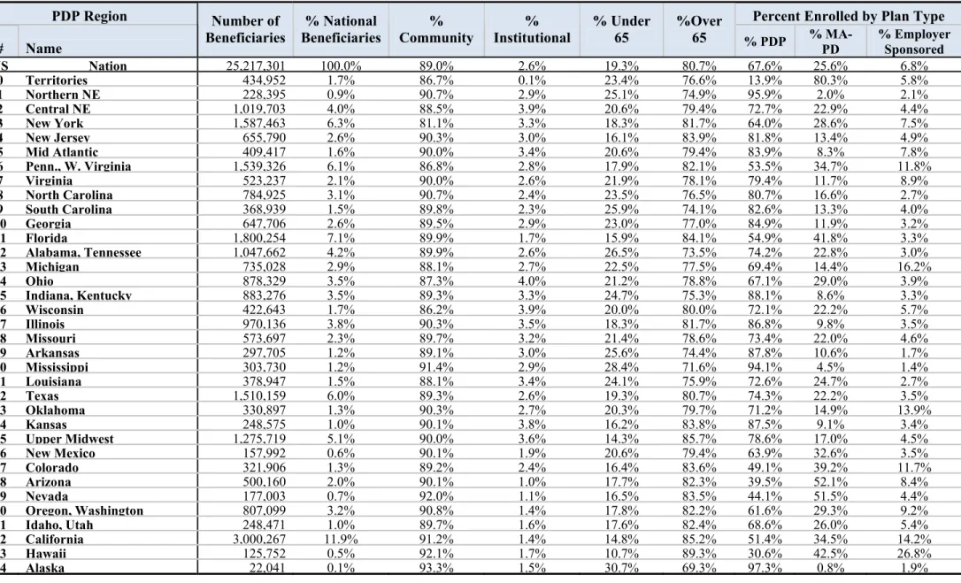
4.1.2. Enrollment by PDP Region and Beneficiary Characteristics ... 36
4.2 Composition of Samples Used to Formulate Price Indices ... 40
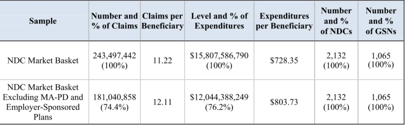
4.2.1. Composition of the NDC and GSN Market Basket Samples ... 41
4.2.2. Restricting Samples to Claims from PDP Plans ... 42
4.2.3. Problems with the Reporting of Quantities in the PDE Data... 44
4.3 Composition of the Sample Used to Measure Utilization of Part D Drugs... 45
4.3.1. Primary Beneficiary Populations Used to Study Utilization ... 45
4.3.2. Composition-Adjusted Variants of these Beneficiary Populations ... 46
5 Patterns of Geographic Variation in the Prices of Part D Drugs... 49
5.1 Regional Price Variation in Ingredient Costs ... 50
5.1.1. Regional Price Indices for Ingredient Costs – NDC Basket... 50
5.2 Regional Price Indices for Ingredient Costs – GSN Basket ... 55
5.3 Regional Price Variation in Ingredient Costs Plus Dispensing Fees... 59
5.3.1. Regional Price Indices for Ingredient Costs Plus Dispensing Fees – NDC Basket.... 59
5.3.2. GSN Regional Price Indices for Ingredient Costs Plus Dispensing Fees ... 63
5.4 Adjustment of Monthly Prices for Possible Inflation During 2007... 66
5.5 Summary of Findings for Regional Price Variation ... 68
6 Patterns of Geographic Variation in Utilization of Part D Drugs... 69
6.1 Differences in Number of Claims Per Capita across Regions and Groups... 69
6.1.1. Per Capita Claims for Overall Part D Population ... 70
6.2 Comparisons of Per Capita Expenditures across Regions and Groups... 75
6.2.1. Differences in Expenditures on Ingredient Costs ... 75
6.2.2. Differences in Expenditures on Ingredient Costs and Dispensing Fees ... 77
6.3 Expenditure Distributions: Controlling for Differences in Regional Risk Factors... 92
6.3.1. Expenditures on Ingredient Costs Adjusting for Population Composition... 93
6.3.2. Expenditures on Ingredient Costs and Dispensing Fees Adjusting for Population Composition... 95
6.4 Regional Variation in Average Per-Beneficiary Expenditures... 101
6.5 Summary of Findings... 105
Bibliography ... 107
Appendix A: Additional Information on Use of PDE Data for Prices... 109
Appendix B: MA-PD Price Index tables... 111
Appendix C: Dispensing Fee Price Index tables ... 121
Appendix D: Additional Utilization tables ... 131
Appendix E: Availability of Best Prices across Counties in Alaska... 167
E.1 Claims ... 168
E.2 Mail Order Prices based on PlanFinder ... 169
LIST OF TABLES AND FIGURES
Table 2.1: Indices Used for Geographic Adjustment in Medicare ... 6
Table 2.2: Number of PDP Contracts in Each PDP Region ... 8
Figure 2.1: Cumulative Costs Paid by Beneficiary and Plan under Standard Benefit Design ... 10
Figure 2.2: Cumulative Amount Paid By Example Beneficiary by High, Low, and Average Cost Region... 12
Figure 2.3: Cumulative Amount Paid by Plan for High, Low, and Average Drug Price Region. 13 Figure 2.4: Relation between National Average Bid, Base Premium and Direct Subsidy... 15
Figure 2.5: Impact of Regional Price Variation on Subsidies and Beneficiary Premiums... 16
Figure 2.6: Beneficiary Premiums and Direct Subsidies with Geographic Adjustment... 17
Table 3.1: Example of a GSN Structure Integrating NDC Products ... 24
Table 4.1: Summary of Enrollment in Part D Program by Region in 2007... 39
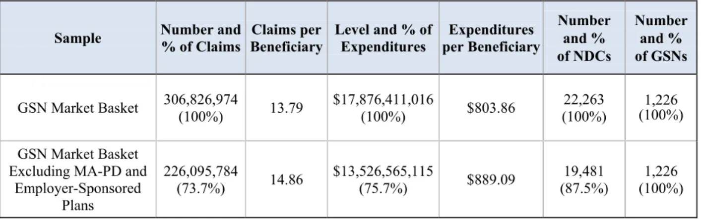
Table 4.2: Effects of Market Basket Selection on Sample Composition of PDEs ... 41
Table 4.3: Composition of the NDC Market Basket Before/After PDP Contract Restriction ... 43
Table 4.4: Composition of the GSN Market Basket Before/After PDP Contract Restriction... 44
Table 5.1: Regional Price Indices Relative to National Indices – Per Unit Ingredient Cost – NDC Basket ... 51
Table 5.2: Regional Price Index Relative to National Median Index – Per Unit Ingredient Cost – NDC Basket... 54
Table 5.3: Regional Price Indices Relative to National Indices – Per Unit Ingredient Cost – GSN Basket ... 57
Table 5.4: Regional Price Index Relative to National Median Index – Per Unit Ingredient Cost – GSN Basket ... 58
Table 5.5: Regional Price Indices Relative to National Indices – Per Unit Ingredient Cost Plus Dispensing Fee – NDC Basket... 60
Table 5.6: Regional Price Index Relative to National Median Index– Per Unit Ingredient Cost Plus Dispensing Fee –NDC Basket ... 61
Table 5.7: Regional Price Indices Relative to National Index – Per Unit Ingredient Cost Plus Dispensing Fee – GSN Basket... 64
Table 5.8: Regional Price Index – Per Unit Ingredient Cost Plus Dispensing Fee – GSN Basket65 Table 5.9: National Inflation Rates by Month for the NDC Market Basket... 67
Table 5.10: National Inflation Rates by Month for the GSN Market Basket ... 67
Table 6.1: All Beneficiaries: Claims Distribution ... 72
Table 6.2: Community Beneficiaries: Claims Distribution ... 73
Table 6.3: Institutional Beneficiaries: Claims Distribution ... 74
Table 6.4: All Beneficiaries: Ingredient Cost Distribution... 80
Table 6.5: All Beneficiaries: Comparison of Ingredient Cost Distributions Regional Statistics Measured Relative to National Values ... 81
Table 6.6: Community Beneficiaries: Ingredient Cost Distribution... 82
Table 6.7: Community Beneficiaries: Comparison of Ingredient Cost Distributions Regional Statistics Measured Relative to National Values... 83
Table 6.8: Institutional Beneficiaries: Ingredient Cost Distribution... 84
Table 6.9: Institutional Beneficiaries: Comparison of Ingredient Cost Distributions Regional Statistics Measured Relative to National Values... 85
Table 6.10: All Beneficiaries: Ingredient Plus Dispensing Cost Distribution... 86
Table 6.11: All Beneficiaries: Comparison of Ingredient Plus Dispensing Cost Distributions Regional Statistics Measured Relative to National Values ... 87
Table 6.12: Community Beneficiaries: Ingredient Plus Dispensing Cost Distribution... 88
Table 6.13: Community Beneficiaries: Comparison of Ingredient Plus Dispensing Cost
Distributions Regional Statistics Measured Relative to National Values ... 89
Table 6.14: Institutional Beneficiaries: Ingredient Plus Dispensing Cost Distribution... 90
Table 6.15: Institutional Beneficiaries: Comparison of Ingredient Plus Dispensing Cost
Distributions Regional Statistics Measured Relative to National Values ... 91
Table 6.16: Community Beneficiaries: Comparison of Ingredient Cost Distributions Adjusting for Population Composition - Regional Statistics Measured Relative to Average Regional Values... 97
Table 6.17: Institutional Beneficiaries: Comparison of Ingredient Cost Distributions Adjusting for Population Composition - Regional Statistics Measured Relative to Average Regional Values... 98
Table 6.18: Community Beneficiaries: Comparison of Ingredient Plus Dispensing Cost
Distributions Adjusting for Population Composition - Regional Statistics Measured Relative to Average Regional Values... 99
Table 6.19: Institutional Beneficiaries: Comparison of Ingredient Plus Dispensing Cost Dispensing Adjusting for Population Composition - Regional Statistics Measured Relative to Average Regional Values... 100
Table 6.20: Regional Variation in Average Per Beneficiary Expenditures for Ingredient Costs Plus Dispensing Fees – Original Levels... 102
Table 6.21: Regional Variation in Average Per Beneficiary Expenditures for Ingredient Costs Plus Dispensing Fees – Original Index... 103
Table 6.22: Regional Variation in Average Per Beneficiary Expenditures for Ingredient Costs Plus Dispensing Fees – Adjusted for Population Composition... 104
Table A.1: PDE Data Elements ... 109
Table B.1: Regional Price Index – Per Unit Ingredient Cost – NDC Basket ... 112
Table B.2: Regional Price Indices Relative to National Index – Per Unit Ingredient Cost – NDC Basket ... 113
Table B.3: Regional Price Index – Per Unit Ingredient Cost – GSN Basket... 114
Table B.4: Regional Price Indices Relative to National Index – Per Unit Ingredient Cost – GSN Basket ... 115
Table B.5: Regional Price Index – Per Unit Ingredient Cost Plus Dispensing Fee – NDC Basket ... 116
Table B.6: Regional Price Indices Relative to National Index – Per Unit Ingredient Cost Plus Dispensing Fee – NDC Basket... 117
Table B.7: Regional Price Index – Per Unit Ingredient Cost Plus Dispensing Fee – GSN Basket ... 118
Table B.8: Regional Price Indices Relative to National Index – Per Unit Ingredient Cost Plus Dispensing Fee – GSN Basket... 119
Table C.2: PDP Regional Price Indices Relative to National Index – Per Claim Dispensing Fee –
NDC Basket... 123
Table C.3: PDP Regional Price Index – Per Claim Dispensing Fee – GSN Basket... 124
Table C.4: PDP Regional Price Indices Relative to National Index – Per Claim Dispensing Fee – GSN Basket ... 125
Table C.5: MA-PD Regional Price Index – Per Claim Dispensing Fee – NDC Basket... 126
Table C.6: MA-PD Regional Price Indices Relative to National Index – Per Claim Dispensing Fee – NDC Basket ... 127
Table C.7: MA-PD Regional Price Index – Per Claim Dispensing Fee – GSN Basket ... 128
Table C.8: MA-PD Regional Price Indices Relative to National Index – Per Claim Dispensing Fee – GSN Basket... 129
Table D.1: All PDP Beneficiaries: Claims Distribution... 133
Table D.2: Community PDP Beneficiaries: Claims Distribution ... 134
Table D.3: Institutional PDP Beneficiaries: Claims Distribution... 135
Table D.4: All MA-PD Beneficiaries: Claims Distribution... 136
Table D.5: Community MA-PD Beneficiaries: Claims Distribution... 137
Table D.6: Institutional MA-PD Beneficiaries: Claims Distribution ... 138
Table D.7: All PDP Beneficiaries: Ingredient Cost Distribution... 139
Table D.8: All PDP Beneficiaries: Comparison of Ingredient Cost Distributions Regional Statistics Measured Relative to National Values... 140
Table D.9: Community PDP Beneficiaries: Ingredient Cost Distribution... 141
Table D.10: Community PDP Beneficiaries: Comparison of Ingredient Cost Distributions Regional Statistics Measured Relative to National Values ... 142
Table D.11: Institutional PDP Beneficiaries: Ingredient Cost Distribution ... 143
Table D.12: Institutional PDP Beneficiaries: Comparison of Ingredient Cost Distributions Regional Statistics Measured Relative to National Values ... 144
Table D.13: All PDP Beneficiaries: Ingredient Plus Dispensing Cost Distribution... 145
Table D.14: All PDP Beneficiaries: Comparison of Ingredient Plus Dispensing Cost Distributions Regional Statistics Measured Relative to National Values ... 146
Table D.15: Community PDP Beneficiaries: Ingredient Plus Dispensing Cost Distribution... 147
Table D.16: Community PDP Beneficiaries: Comparison of Ingredient Plus Dispensing Cost Distributions Regional Statistics Measured Relative to National Values ... 148
Table D.17: Institutional PDP Beneficiaries: Ingredient Plus Dispensing Cost Distribution... 149
Table D.18: Institutional PDP Beneficiaries: Comparison of Ingredient Plus Dispensing Cost Distributions – Regional Statistics Measured Relative to National Values ... 150
Table D.19: All MA-PD Beneficiaries: Ingredient Cost Distribution ... 151
Table D.20: All MA-PD Beneficiaries: Comparison of Ingredient Cost Distributions Regional Statistics Measured Relative to National Values... 152
Table D.21: Community MA-PD Beneficiaries: Ingredient Cost Distribution ... 153
Table D.22: Community MA-PD Beneficiaries: Comparison of Ingredient Cost Distributions Regional Statistics Measured Relative to National Values ... 154
Table D.23: Institutional MA-PD Beneficiaries: Ingredient Cost Distribution... 155
Table D.24: Institutional MA-PD Beneficiaries: Comparison of Ingredient Cost Distributions Regional Statistics Measured Relative to National Values ... 156
Table D.25: All MA-PD Beneficiaries: Ingredient Plus Dispensing Cost Distribution ... 157
Table D.26: All MA-PD Beneficiaries: Regional of Ingredient Plus Dispensing Cost
Distributions Regional Statistics Measured Relative to National Values ... 158
Table D.27: Community MA-PD Beneficiaries: Ingredient Plus Dispensing Cost Distribution ... 159
Table D.28: Community MA-PD Beneficiaries: Comparison of Ingredient Plus Dispensing Cost Distributions Regional Statistics Measured Relative to National Values ... 160
Table D.29: Institutional MA-PD Beneficiaries: Ingredient Plus Dispensing Cost Distribution161
Table D.30: Institutional MA-PD Beneficiaries: Comparison of Ingredient Plus Dispensing Cost Distributions Regional Statistics Measured Relative to National Values ... 162
Table D.31: Community PDP Beneficiaries: Comparison of Ingredient Cost Distributions Adjusting for Population Composition - Regional Statistics Measured Relative to Average Regional Values ... 163
Table D.32: Institutional PDP Beneficiaries: Comparison of Ingredient Cost Distributions Adjusting for Population Composition - Regional Statistics Measured Relative to Average Regional Values ... 164
Table D.33: Community PDP Beneficiaries: Comparison of Ingredient Plus Dispensing Cost Distributions Adjusting for Population Composition - Regional Statistics Measured Relative to Average Regional Values... 165
Table D.34: Institutional PDP Beneficiaries: Comparison of Ingredient Plus Dispensing Cost Distributions Adjusting for Population Composition - Regional Statistics Measured Relative to Average Regional Values... 166
Table E.1: Enrollment of PDP Beneficiaries by County in Alaska, 2007 ... 168
Table E.2: Availability of GSNs at Best Prices in All Counties for GSNs Purchased in at Least Three Counties According to PDE Data... 169
Table E.3: Availability of GSNs at Best Prices ... 170
1 INTRODUCTION
In 2003, the Medicare Prescription Drug Improvement and Modernization Act (MMA) mandated the creation of a voluntary program for prescription drugs within Medicare,
administered by the Centers for Medicare and Medicaid Services (CMS). Described as the “most important health care legislation passed by Congress since the enactment of Medicare and Medicaid in 1965,”1 the drug benefit filled a critical gap in Medicare coverage. The Part D program, launched on January 1, 2006, covered 24.2 million beneficiaries by 2007. Through CMS, the Part D program pays a direct subsidy to Part D plans, equal to a plan’s risk-adjusted bid for a standardized benefit package minus the beneficiary’s base premium for the standard package.
In establishing the prescription drug benefit, the MMA allowed for adjustments in the direct subsidy to account for geographic variation in prices, unless the geographic differences are too minimal to justify such an adjustment. To be specific, Section 1860D-15(c)(2) specifies the following:
a. In general.—Subject to subparagraph (B), for purposes of section 1860D-13(a)(1)(B)(iii), the Secretary shall establish an appropriate methodology for
adjusting the national average monthly bid amount (computed under section 1860D-13(a)(4)) to take into account differences in prices for covered part D drugs among PDP regions.
b. De minimis rule.—If the Secretary determines that the price variations described in subparagraph (A) among PDP regions are de minimis, the Secretary shall not provide for adjustment under this paragraph.
c. Budget neutral adjustment.—Any adjustment under this paragraph shall be applied in a manner so as to not result in a change in the aggregate payments made under this part that would have been made if the Secretary had not applied such adjustment. Section 107 of the MMA mandates that the Secretary conduct a study on the “regional variations in prescription drug spending.” Specifically, in examining the variation in per capita Part D drug spending among the 34 prescription drug plan (PDP) regions, the legislation states:
1Altman, D. 2004. “The New Medicare Prescription-Drug Legislation”.
New England Journal of Medicine. Vol
350, no.1 (January):9-10.
1. In general.--The Secretary shall conduct a study that examines variations in per capita spending for covered part D drugs under part D of title XVIII of the Social Security Act among PDP regions and, with respect to such spending, the amount of such variation that is attributable to
A. price variations (described in section 1860D-15(c)(2) of such Act); and B. differences in per capita utilization that is not taken into account in the
health status risk adjustment provided under section 1860D-15(c)(1) of such Act.
2. Report and recommendations.--Not later than January 1, 2009, the Secretary shall submit to Congress a report on the study conducted under paragraph (1). Such report shall include
A. information regarding the extent of geographic variation described in paragraph (1)(B);
B. an analysis of the impact on direct subsidies under section 1860D-15(a)(1) of the Social Security Act in different PDP regions if such subsidies were adjusted to take into account the variation described in subparagraph (A); and
C. recommendations regarding the appropriateness of applying an additional geographic adjustment factor under section 1860D-15(c)(2) that reflects some or all of the variation described in subparagraph (A).
In response to this mandate in the MMA, this report investigates regional variation in per capita expenditure on covered Part D drugs and Part D drug prices as reported in prescription drug event (PDE) data submitted by prescription drug plans. In particular, we address four key questions:
(1) How much did Part D drug prices vary across the 34 PDP regions in 2007? (2) How much did utilization of prescription drugs vary by region?
(3) How much did per capita spending on prescription drugs vary by region?
(4) How much did per capita spending on drugs vary by region, after accounting for health status risk adjustment and price variation?
Answers to these four questions provide the basis for determining the appropriateness of applying a geographic adjustment factor to Part D subsidies.
The report is structured as follows: as background to the analysis, Section 2 reviews the use of geographic adjustments in the Medicare program, the role of the 34 PDP regions, and how regional adjustments would interact with the Part D benefit framework. Section 3 describes the methodology for measuring price variation for prescription drugs as well as measuring variation
Geographic Variation in Drug Prices and Spending in the Part D Program | August 2009 3 in utilization as measured by per capita spending. In Section 4, we describe the data we use for the analysis, including the samples of beneficiaries and drug products. The key results are divided into two sections. Section 5 presents the patterns of geographic variation in the prices of Part D drugs, and Section 6 presents the comparable patterns for utilization, before and after accounting for health status.
2 BACKGROUND
The concept of geographic adjustment was a natural consideration for the Part D program because other components of Medicare include geographic adjustments. In this section, we first review the use of geographic adjustments to account for differences in input prices within these other sectors of the Medicare program. The second section reviews the role of regions in the design of Part D. We then consider how differences in drug prices would affect beneficiaries and plans given each major payment aspect of the Part D program. In doing so, we also demonstrate the expected impacts of introducing a geographic adjustment to account for such price differences. Finally, we briefly discuss whether or not one would expect drug prices to vary by region.
2.1 Existing Geographic Adjustments in the Medicare Program
Geographic adjustments are currently applied to provider payments in Medicare Part A, the Hospital Insurance Program (covering inpatient care, skilled nursing facilities, home health and hospice care), and in Part B, the Supplementary Medical Insurance Program (covering physician, outpatient, home health, preventative services and durable medical equipment). Under these programs, providers are reimbursed on a fee-for-service basis at payment rates established by CMS. The base reimbursement rates represent national average reimbursement rates. Budget neutral geographic adjustments then scale these average payments up in areas with high input costs and down in areas with low input costs.
The geographic adjustments in Part A and B are based on measures of the costs of inputs for services. The hospital wage index, the key geographic index used in Part A, is designed to capture the relative wage level for hospital staff in a given area, compared to national average hospital wages. It adjusts only the labor portion of the reimbursement rate. Physician payments under Part B are adjusted using three separate indices, known as Geographic Practice Cost Indices (GPCIs). These indices are designed to account for differences in the relative cost of
physician wages, practice expenses (employees, office rents, and supplies) and malpractice premiums as different inputs into outpatient physician services.2
The geographic adjustments in Part A and B offset costs for providers, not for
beneficiaries. Because the adjustments change the reimbursement rates for providers, they also change the cost of co-payments for beneficiaries for services that require beneficiaries to pay a share of costs. For example, most Part B services, including physician visits, require a 20 percent co-insurance, so when the geographic adjustment increases (or decreases) provider reimbursements, it also increases (or decreases) beneficiary costs.
The 2007 values for the hospital wage index and the GPCIs are shown in Table 2.1. Conceptually, these indices are all normalized around 1.0. For hospitals, to take an example, the index multiplies the labor portion by as much as 1.54 (a 54 percent increase or as little as 0.71 (a 29 percent decrease). The greatest variation is seen in the malpractice GPCI for physician payments, although this applies on average to only 4 percent of a physician’s reimbursement rate. The lowest variation, from 1.0000 to 1.0830, occurs in the physician work GPCI, but largely because, by law, this variation is reduced to one-fourth of the original variation, and through 2007, a floor of 1.0 was also imposed, so there were only upward adjustments.
Table 2.1: Indices Used for Geographic Adjustment in Medicare Geographic Adjustment
Indices 2007 Part Minimum Value Maximum Value Standard Deviation
Hospital Wage Index* A 0.708 1.542 0.155
Physician Work GPCI B 1.000 1.083 0.020
Practice Expense GPCI B 0.699 1.546 0.168
Malpractice GPCI B 0.257 2.700 0.416
* Pre-reclassification index; the reported standard deviation is calculated across hospitals, not regions.
2The hospital wage index or a variant of it is also used for skilled nursing facilities, home health care, and hospice
2.2 Role of Regions in Part D
Regions play a different role in Part D than they do in Parts A and B, where regions are largely used to distinguish higher and lower input cost areas. Instead of relying on payment rates established by CMS, Part D payments are based on competitive bids submitted by drug plans in each of the 34 PDP regions. Beneficiaries choose among plans available in their region, based on plans’ premiums, drug costs and drug formularies. The PDP regions were defined with the intention that at least two plans participate in each region. Regions were also designed to adhere as closely as possible to MA regions and to group states with similar levels of drug spending.3
By 2007, beneficiaries were participating in 90 PDP contracts with about 1,900 plan options and 545 MA-PD contracts with about 2,400 plan options. The Table below (2.2) displays the total number of contracts offered in each region; as Table 2.2 shows, at least 41 contracts and as many as 75 contracts were offered in each PDP region. 4
Under the competitive bidding process, Part D shows substantial variation in beneficiary premiums across regions. In 2007, the average beneficiary premiums for standard coverage, calculated by CMS, ranged from $20.56 per month in Nevada to $33.56 per month in Alaska.5
Total costs for beneficiaries can vary much more. An earlier study on geographic variation published in the Journal of General Internal Medicine (Davis 2007) examined differences in projected total plan costs (including both premiums and drug expenditures) for the lowest cost plans available in each state. Focusing on four example cases, the authors found costs ranging from half of the national average to more than double the national average, with greater variation among higher cost individuals.
This regional variation in premiums is not surprising, since geographic variation in prescription drug spending was known prior to the start of the Part D program. Analyses summarized by the Medicare Payment Advisory Commission (MedPAC) found geographic
3 See MedPAC 2005.
4Whereas plans are the specific insurance options beneficiaries may choose from, contracts are the different
companies offering the plans. Contracts may offer numerous plans in one region and may also offer the same plan in different regions. Note, each time the same plan is offered in a different PDP region it is considered a new plan option.
5These average premiums are calculated by CMS to set regional benchmarks for low-income subsidies.
differences in spending ranging from 120 percent of the national average in the Northeast to less than 80 percent of the national average in the West. This variation encompasses differences in
Table 2.2: Number of PDP Contracts in Each PDP Region PDP Region
Code PDP Region Name State(s) Number of Contracts
01 Northern New England Maine New Hampshire 56
02 Central New England Connecticut, Massachusetts, Rhode Island,
Vermont 72
03 New York New York 73
04 New Jersey New Jersey 65
05 Mid-Atlantic Delaware, District of Columbia, Maryland 68 06 Pennsylvania, West Virginia Pennsylvania, West Virginia 69
07 Virginia Virginia 69
08 North Carolina North Carolina 69
09 South Carolina South Carolina 66
10 Georgia Georgia 68
11 Florida Florida 75
12 Alabama, Tennessee Alabama, Tennessee 67
13 Michigan Michigan 66
14 Ohio Ohio 75
15 Indiana, Kentucky Indiana, Kentucky 68
16 Wisconsin Wisconsin 57 17 Illinois Illinois 69 18 Missouri Missouri 60 19 Arkansas Arkansas 54 20 Mississippi Mississippi 57 21 Louisiana Louisiana 60 22 Texas Texas 70 23 Oklahoma Oklahoma 58 24 Kansas Kansas 52
25 Upper Midwest and Northern Plains Iowa, Minnesota, Montana, Nebraska, North Dakota
South Dakota, Wyoming 66
26 New Mexico New Mexico 50
27 Colorado Colorado 57
28 Arizona Arizona 65
29 Nevada Nevada 61
30 Oregon, Washington Oregon Washington 65
31 Idaho, Utah Idaho, Utah 52
32 California California 72
33 Hawaii Hawaii 43
beneficiaries’ health status, income and insurance coverage, as well as differences in the number of providers, providers’ prescribing patterns and drug prices.6 A number of researchers have
documented comparable variation in expenditures per capita in the fee-for-service components of Medicare. A review of these studies by the Congressional Budget Office (2008) concluded that prices of medical services and beneficiary health status together explain less than half of the total variation in fee-for-service expenditures.
2.3 Expected Impact of Higher Regional Drug Prices on Part D
Part D premiums by region are driven by a complex set of factors, including the expected utilization of drugs based on the preferences and health status of beneficiaries, tradeoffs between premiums and co-payments, and competitive forces within regions, as well as differences in the price of the prescription drug products. Since a regional adjustment would specifically address the differences associated with prices, any potential adjustment must be understood within the context of the Part D benefit design. In this subsection, we review the major elements of the Part D benefit and payment structures, and consider how higher or lower drug prices would impact beneficiaries and plans given these structures. There are three main elements of the Part D framework to analyze in the context of geographic differences in prices: the standard benefit design, the direct subsidy and associated beneficiary premiums, and the low income subsidy. Other aspects of the Part D payments, such as risk corridors, should not significantly differ between high price and low price regions.
2.3.1. Standard Benefit Design
The MMA mandates a minimum “standard” benefit package for Part D coverage. Although plan sponsors may offer a variety of plans, which can include plans that provide enhanced coverage, they must include a price bid that reflects this standard benefit design. Intended to balance beneficiary coverage with incentives to avoid the overutilization of prescription drugs, the standard benefit structure includes four separate coverage bands.
Figure 2.1 illustrates the four coverage bands for a beneficiary paying $500 per month in prescription drug costs, with coverage bands shown for the 2007 plan year. The shaded areas
6 See MedPAC 2005.
together represent the total costs of the drugs; by the end of the year this beneficiary would incur $6,000 in total drug expenditures, with costs shared between the beneficiary, the plan, and CMS. In the first band, the beneficiary covers the initial costs through a deductible, set at $265. For the total drug costs between $265 and $2400, the plan pays 75 percent of the total costs, and the beneficiary pays 25 percent. This second phase is referred to as the Initial Coverage Level. The third phase is the “coverage gap.” For total drug costs between $2,400 and $5,451, the standard Part D benefit offers no additional coverage. Above $5,451 in total costs, which is equivalent to $3,850 in beneficiary out-of-pocket costs, Part D offers catastrophic coverage. In this phase, CMS pays 80 percent of drug costs, the beneficiary pays 5 percent, and the plan pays the remaining 15 percent.
together represent the total costs of the drugs; by the end of the year this beneficiary would incur $6,000 in total drug expenditures, with costs shared between the beneficiary, the plan, and CMS. In the first band, the beneficiary covers the initial costs through a deductible, set at $265. For the total drug costs between $265 and $2400, the plan pays 75 percent of the total costs, and the beneficiary pays 25 percent. This second phase is referred to as the Initial Coverage Level. The third phase is the “coverage gap.” For total drug costs between $2,400 and $5,451, the standard Part D benefit offers no additional coverage. Above $5,451 in total costs, which is equivalent to $3,850 in beneficiary out-of-pocket costs, Part D offers catastrophic coverage. In this phase, CMS pays 80 percent of drug costs, the beneficiary pays 5 percent, and the plan pays the remaining 15 percent.7 In the example presented in Figure 2.1, the beneficiary’s total annual
out-of-pocket cost (not including the premium) is $3,877.
Figure 2.1: Cumulative Costs Paid by Beneficiary and Plan under Standard Benefit Design Example Beneficiary with $500 per Month in Prescription Drug Expenditures
7The 80% contribution by CMS, referred to as reinsurance, may be reduced by the difference between the gross
costs of covered drugs and the net amount actually paid by plans, accounting for discounts, rebates and other savings provided by drug manufacturers, pharmacies, etc.
Effect of Price Differences on Beneficiary Out-of-Pocket Payments
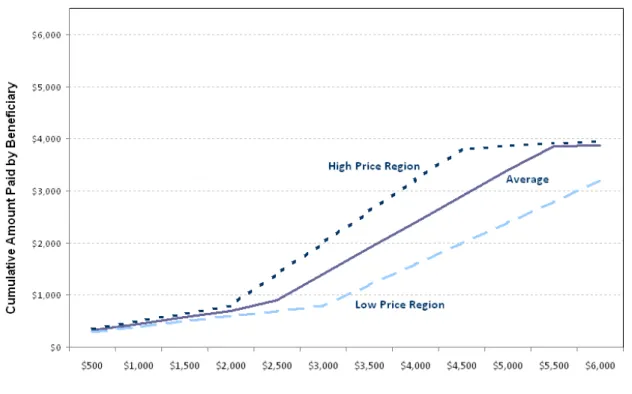
If there are regional differences in drug prices, the beneficiary illustrated in Figure 2.1 could face higher or lower annual costs. The solid line in Figure 2.2 presents the beneficiary share from Figure 2.1. Assuming this beneficiary’s $500 per month drug costs represent the costs at national average prices, the other two lines illustrate how these costs would differ in a region with higher or lower drug prices. The top line represents the total cumulative amount this beneficiary would pay if the price for the same drugs was $600 instead of $500. The lower line represents the amount the beneficiary would pay if the price of these drugs was $400.
Because our beneficiary reached the catastrophic level when paying the national average price for these drugs, the additional costs he would face in a high cost region are small.
Although the total drug costs would be $7,200 per year in a high cost region instead of $6,000, his additional out-of-pocket costs are only $60, which is equal to 5 percent of this added cost. On the other hand, if he resided in the low cost region, his cumulative costs would be $678 lower than if he were paying the national average price, because he is still in the coverage gap at the end of the year, paying the full costs of his drugs himself.
Figure 2.2: Cumulative Amount Paid By Example Beneficiary by High, Low, and Average Cost Region
Although the catastrophic coverage level protects high expenditure beneficiaries in high cost areas, beneficiaries whose total drug expenditures place them in the coverage gap pay the entire additional prices for their drugs in high cost regions. If our example beneficiary had faced the same prices but taken half the drug quantity, his drug costs would total $250 per month or $3,000 annually in the average area. It would now take him until December to hit the total costs that he previously reached in June. At the end of the year, he would have paid $1,399 total. If he lived instead in a high price region, both the total drug costs he incurred and his total out-of-pocket costs would be $600 higher. That is, in the high cost region, he would pay $1,999 of the total cost of $3,600. Similarly, he would capture all of the savings from the lower prices in a cheaper region, and pay only $799 out of the $2,400 total costs.
Effect of Price Differences on Plan Payments for Drugs
Since the plans pay for the drug expenditures not covered by beneficiaries – except in the catastrophic range where CMS pays most of the costs – it is not surprising that the situation is
largely a mirror image for the plans compared to the beneficiaries. The “average” line in Figure 2.3 graphs the plan costs from Figure 2.1. The higher and lower lines then demonstrate how these plan costs would differ in a high price region and a low price region. Plans are most
Figure 2.3: Cumulative Amount Paid by Plan for High, Low, and Average Drug Price Region
affected by higher prices for beneficiaries whose cumulative drug costs fall into the initial coverage level. If a beneficiary’s cumulative annual expenditures fall into the coverage gap, the costs to plans are not affected by the price of drugs. Plans do not pay any of the cost in the coverage gap, and the cutoff point for the gap is the same for high price as for low price areas. So the total amount paid by plans is the same, about $1,600, whether a beneficiary’s annual expenditures are $2,400 or $5,400. Plans’ costs increase again under catastrophic coverage, but they bear only 15 percent of the price difference in this range, with CMS carrying 80 percent of the total drug costs within this range.
2.3.2. Plan Bids, Beneficiary Premiums and the Direct Subsidy
The cost structure faced by plans (shown in Figure 2.2) is critical in determining the plan bids. Essentially, the plan bids reflect the plans’ predictions of the distribution of beneficiaries’ total drug costs, applying the benefit design rules to determine the implications for plan costs. The bid is thus an estimation of the cost of coverage for the average beneficiary.8 If
beneficiaries’ expenditures fall in either the initial coverage range or the catastrophic coverage range, plans facing higher prices will need to increase their bids. Although bids will differ from plan to plan, on average, regions with higher prices will have higher average plan bids, and regions with lower prices will have lower average plan bids.
As currently structured within Part D, the direct subsidy to plans is based on the national average standard bid, which is a weighted average of the standardized bid amounts submitted by each plan.9 Before adjustments for reinsurance, the base beneficiary premium is 25.5 percent of the national average bid. Ignoring the issue of risk adjustment, the direct subsidy is then
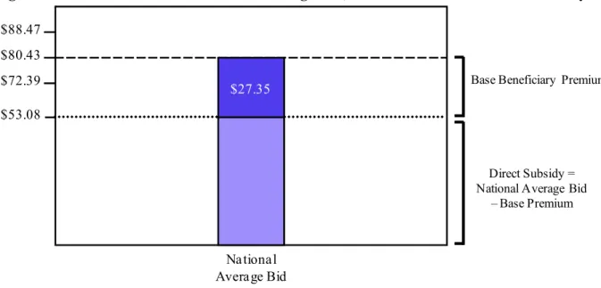
calculated as the national average bid amount minus the beneficiary base premium. For 2007, the beneficiary base premium was $27.35. Given the reinsurance adjustment, this was 34 percent of the national average bid amount of $80.43. Figure 2.4 presents the simple case for a standardized bid at the national average for 2007, where there is no risk adjustment.
The premium actually paid by the beneficiary and the direct subsidy received by the plan will both differ from case to case. For a specific plan, the beneficiary premium is equal to the base beneficiary premium plus the difference between the plan bid and the national average bid. For a bid equal to the national average, the beneficiary premium equals the beneficiary base premium. Plans with bids below the national average will have lower premiums; plans with bids above the national average will have proportionally higher premiums. Plans, in turn, will receive higher direct subsidies for beneficiaries with greater anticipated health needs, provided as an increment to the standardized plan bid, based on a beneficiary specific risk score.
8 MA-PDs submit one bid for Parts A and B, and one for Part D, where the Part D bid is net of any MA rebates that
plans propose to apply to Part D premiums. Bids represent monthly amounts.
Figure 2.4: Relation between National Average Bid, Base Premium and Direct Subsidy
Direct Subsidy = National Average Bid
– Base Premium $27.35 National Average Bid $72.39 $88.47 $80.43 $53.08
Base Beneficiary Premium
In the absence of geographic adjustment in Part D, the direct subsidy is the same for high price regions and low price regions. Because, all else being equal, we would expect high price regions to have bids above the national average, this means that the additional regional costs are passed on to the beneficiaries through higher premiums, as shown in Figure 2.5. In this example, the higher prices result in a 10 percent higher expected cost per beneficiary, compared to the national average bid. Because the direct subsidy is fixed at $53.08, the beneficiary pays all the difference through the higher premium of $35.39 instead of $27.35. Similarly, savings in lower price regions will be passed along to beneficiaries, as lower premiums.
Figure 2.5: Impact of Regional Price Variation on Subsidies and Beneficiary Premiums
Base Beneficiary Premium
$72.39 $88.47 $80.43
$15.50
$53.08$25.50
$35.50
National Average Low Price RegionAverage Plan High Price Region Average Plan
$15.50
$25.50
$35.50
$27.35 $35.39
$19.31
Direct Subsidy = National Average Bid
– Base Premium
2.4 The Potential Role of Geographic Adjustment in Part D
As called for in the MMA, geographic adjustment for higher drug prices would be implemented as an adjustment to the national average bid amount. Abstracting from the exact way this adjustment would be calculated, we would expect the adjustment to scale up the national average bid amount – and by extension, the direct subsidy – in high price regions, and scale down the bid and direct subsidy amounts in low price regions. The discussion presented in Section 2.3 suggests the expected effects of such an adjustment on the costs paid by plans and beneficiaries.
The geographic adjustment would have no direct effect on the overall drug expenditures paid by beneficiaries and plans shown in Figures 2.1 through 2.3. In particular, beneficiaries would still face higher out-of-pocket costs in higher priced areas, since neither the drug prices nor the thresholds in the standard benefit design would be affected by the geographic adjustment. Similarly, the geographic adjustment would not change the costs faced by plans under these expenditures. Because these costs would not be changed, we would not expect the plan bids to change.
The primary effect of the geographic adjustment would occur through the calculation of the direct subsidy and by extension the beneficiary premiums. Since plan bids would still reflect the costs of the drugs, the plan bids would be the same, but the direct subsidy payable to plans in
high price regions would rise. Consequently, given budget neutrality, the direct subsidy for plans in low price regions would fall.
As shown in Figure 2.6, the change in direct subsidies would directly impact the
premiums paid by beneficiaries. Without the adjustment (as shown in Figure 2.5), beneficiaries in low price areas pay lower premiums on average, because their plans were generally below the national average bid. With the geographic adjustment, the beneficiary premiums are evened out across areas. (Figure 2.6 assumes the geographic adjustment would fully adjust for the price differences; however, the Part D adjustment could be applied as only a partial adjustment.) This mechanism is quite different from that seen in Parts A and B, where the geographic adjustments increase the reimbursements to providers in high input cost areas, but also increases costs to beneficiaries in these areas.
Figure 2.6: Beneficiary Premiums and Direct Subsidies with Geographic Adjustment
Avg. Plan Premium
National Average Low Price Region
Average Plan High Price Region Average Plan
$25
$25
$27.35$25
$27.35 $27.35 Avg. Direct Subsidy $72.39 $88.47 $80.43 $53.08In 2007, 9.5 million or 39 percent of PDP and MA-PD Part D enrollees qualified for a low-income subsidy. Because the low-income subsidies generally protect beneficiaries from regional price differences, the geographic adjustment would also have minimal effect on these individuals. Since the beneficiary premiums would even out across regions, the regional benchmarks would also even out. Those beneficiaries paying for premiums on a sliding scale would see their premiums change, with premiums rising for beneficiaries in low price regions (compared to the no-adjustment premium) and falling for beneficiaries in high price regions. As
with other beneficiaries, low-income beneficiaries paying 15 percent coinsurance would not see any change in their out-of-pocket costs on prescriptions.
2.5 Expectations on Geographic Variation in Part D Drug Prices
For the purposes of this discussion, we have assumed that Part D drug prices would vary regionally. However, before we turn to the empirical investigation of regional variation in drug prices, there are two facts to keep in mind. First, there are reasons to believe that Part D drug prices are less likely to vary by locality than are the input costs addressed in the geographic adjustments in Medicare Parts A and B. Second, a focus solely on the drug prices reported as expenditures in the program may miss the full picture of drug costs under Part D.
At the point of sale, Part D drug costs include the ingredient cost and the pharmacist’s dispensing fee (plus sales tax). Because the ingredients are provided through drug
manufacturers, the ingredient costs may be similar to physician office equipment or laboratory services, which under Part B are not geographically adjusted because Medicare assumes a national market. Indeed, at least by mail order, there is a national market for prescription drugs. While dispensing fees may capture regional differences in the costs of pharmacies, mail order pharmacies, large national retail chains, pharmacy benefit managers and wholesale distributors are all likely to dampen geographic differences. Moreover, competitive bidding and the sheer number of drug plans may drive prices down to a common level, especially since many of the plans are national or offered in a number of regions. To date, however, the empirical evidence is mixed. Whereas ASPE (2000) finds substantial geographic variation in drug prices for cash customers but less variation for insured customers, MedPAC (2005) cites several studies showing little or no variation in drug prices across regions.
As noted in the ASPE study, a fundamental challenge in studying drug prices is that the point-of-sale price is not the final price to the plans. Plans receive price discounts both at the time of sale, which would be accounted for in the listed price, and in the form of manufacturer rebates tied to the volume of sales.10 These rebates are considered as part of the total plan costs
10 See Avalere Health LLC, “Follow the Dollar: Understanding Drug Prices and Beneficiary Costs under Medicare
Geographic Variation in Drug Prices and Spending in the Part D Program | August 2009 19 in setting the bids, and the total value of these rebates are determined as part of the end of the year reconciliation with CMS. However, rebates are not reported for individual drugs, so the actual price to plans is not observable. Since the rebates cannot be traced to specific drugs or to individual beneficiaries, they cannot be considered as part of the regional price variation.
2.6 Summary
Geographic adjustments are used in Medicare Parts A and Part B to adjust fee-for-service reimbursement rates for higher input costs faced by providers in high wage, high rent or high malpractice premium areas. These adjustments, which encompass ranges as broad as 0.257 to 2.700 (for malpractice premiums) and as narrow as 1.000 to 1.083 (for physician wages), are applied only to specific portions of the service costs. Costs for goods that are assumed to be purchased on national markets, such as physician office equipment or oxygen tanks, are not adjusted. Most notably, beneficiaries in high cost areas bear some of the costs of these adjustments through higher coinsurance costs.
Unlike Part A and B, if prescription drug prices under Part D differ by region, the additional costs will be borne by beneficiaries rather than the Part D providers. Because of the four-phase basic benefit structure under Part D, beneficiaries may or may not face higher out-of-pocket costs for their prescription drug purchases in areas with higher drug prices, depending upon their annual level of drug spending. Similarly, the additional costs faced by plans in high price areas differ depending on the level of total expenditures. However, plan bids are designed to capture plan costs. Since the direct subsidies are based on national average bid amounts, the subsidy will cover a smaller share of the bid in high drug price areas, and beneficiaries will pay the additional costs in the form of higher premiums. Geographic adjustments would equalize beneficiary premiums across areas with little change in the plan bids, plan costs or beneficiary out-of-pocket costs.
3 METHODOLOGY FOR MEASURING GEOGRAPHIC VARIATION IN DRUG PRICES AND UTILIZATION
The empirical approach for this study is designed to assess the extent of variation in drug prices, claims and spending across PDP regions and to understand the underlying sources of any such geographical variation. The ultimate goal is to determine whether and what geographic adjustments to Part D direct subsidies might be appropriate. In undertaking this empirical analysis, however, there are significant challenges to overcome. The most problematic challenges arise in defining regional prices, given that prices vary within regions as well as across regions, and in defining what constitutes a “drug.” Beyond these core challenges,
beneficiary choices intricately shape both Part D prices and consumption. Beneficiaries not only select freely among a wide variety of plans – each offering its own tailored menu of drugs and prices – but also face varying cost sharing tiers that influence their decisions about the particular drugs and drug quantities they consume. Any analysis must neutralize the influence of these choices to isolate the variation that would be the focus of geographic adjustment policies.
Our empirical design builds on analytical steps formulated to distinguish two sets of factors that jointly determine Part D prices and quantities: the opportunities available to beneficiaries – which might be addressed with policy changes – and the choices made by
beneficiaries that lead to the observed outcomes. The analytical steps first address the following three questions:
Step 1: How much do drug prices vary across regions and plans?
Step 2: What differences arise in the utilization of pharmaceuticals across regions and beneficiary groups?
Step 3: To what extent are there regional variations in utilization that are not caused by differences in health status and prices?
Depending on the answers to these questions, there are two potential additional steps:
Step 4: If prices vary, what do the patterns of utilization and geographic differences in Part D costs imply about policy options for adjusting direct subsidies by region? Step 5: What will be the impact on the direct subsidy if subsidies are adjusted for price
variation?
This section describes our statistical design for implementing Steps 1 through 3. The first analysis step addresses how opportunities in drug prices differ across regions, as measured
through price indices. The first subsection presents a basic price index and discusses the
underlying challenges entailed in formulating price indices and utilization measures for a market as complex as the one applicable for drugs. We then describe our procedures for defining drug products and the complexity of assigning prices. Subsection 3.4 presents constructions of price indices designed to reveal underlying differentials in drug prices across regions. Given this background, Section 3.5 presents our approach for Steps 2 and 3. This subsection describes the metrics we use measure regional differences in the utilization of drugs, including an overview of our strategy to control for health status in examining regional variations in expenditures.
3.1 The Standard Price Index and Challenges in Constructing Price Indices for Drugs
A geographic price index relates a “quantity” weighted average of regional “prices” of individual products by region to the corresponding weighted average of national “prices.” The weights used in this construction remain “fixed” in that they differ across products but stay constant across regions. More specifically, a fixed-weight geographic price index for region r takes the form:
(3.1)
i r i iN kN kN k r i iN i rW
p
p
q
p
q
P
)
(
)
(
where)
(
kN kN k iN iNp
q
q
W
designates the weights used to evaluate the price index; pir refers to the price of product i in
region r; piN represents the price of product i nationally; and qiN denotes the (national) quantity
associated with product i. Two popular formulations of this index include the Laspeyres and
Paasche price indices, which merely differ in the way one sets the weights WiN. The
denominator of (3.1) sums prices and quantities over all products i; we use k in the denominator
to flag that there are alternative ways to set the weights, depending on the particular formulation. We describe the weights, along with the other components below.
In a market as complex as the market for drugs, one must make decisions about four components that make up the index. First, one must select the geographic areas over which one measures drug units and prices used to construct the index. For this analysis, these geographic areas are the defined PDP regions. Second, one must establish the definition of drug products. Third, one must consider the appropriate notion of prices for the drug products. The theory motivating the formulation and interpretation of price indices maintains the assumptions that products are well defined and each of these products have a single price during the relevant time period. As further explained below, neither of these assumptions applies in the market for pharmaceuticals. Finally, one must establish the product shares that determine the fixed weights.
To carry out Step 1 and Step 2 of our study, therefore, an analytical approach must address the following key questions in constructing a price index:
What is the definition of a drug product?
What is an appropriate basket of goods to include in the indices?
What are the appropriate prices to consider?
How are the fixed weights constructed?
3.2 Definition of Drug Products in Part D Data
The first analytical challenge is defining what constitutes drug products. There are tens of thousands of drugs listed by their unique National Drug Codes or NDCs. A drug’s NDC consists of an eleven-digit code, with the first five numbers indicating the labeler code (FDA assigned), the next four numbers registering the drug, dosage form and strength (manufacturer assigned), and the remaining two numbers signifying the package size (manufacturer assigned). Even a brand name drug may have many different NDCs. In this analysis, we consider both individual NDCs and groupings of NDCs mapped into categories of “comparable” products. Two basic approaches exist for defining comparability: the first aggregates NDCs into higher level therapeutic classifications, which interprets drugs used to treat similar medical conditions as substitutes; and the second groups NDCs according to their chemical makeup (Generic Sequencing Number or GSN). We use the second approach to group NDCs in this analysis.
3.2.1. Information in the Part D Data
Part D plans submit Prescription Drug Event (PDE) data to CMS to report details of all their transactions documenting the dispensing of Part D drugs. Each PDE claim discloses the NDC of the drug, its ingredient cost, the quantity purchased, date of the sale, the plan covering the purchase, and the pharmacy where the drug was obtained. Combining these PDE data with information about plan characteristics from CMS’s Health Plan Monitoring System (HPMS) data and about attributes of drug products from First DataBank (FDB) allows one to determine: (i) the therapeutic classification and chemical makeup of the NDC purchased, (ii) the region and specific local pharmacy where a given drug was sold, (iii) reference units and prices used to sell the NDC (e.g. the NDC’s average wholesale price (AWP) and average manufacturer price (AMP)), and (iv) information about the other costs the beneficiary and plan had to pay to acquire that drug, such as the benefit cost structure of the plan.
3.2.2. Classifying Drugs by Their Generic Sequence Numbers (GSNs)
The National Council for Prescription Drug Programs (NCPDP) offers a typology for allotting NDCs into broader categories termed Generic Sequence Numbers (GSNs), which also serves as the standard used by FDB. A GSN identifies pharmaceutically identical NDCs. More precisely, a drug’s assigned GSN maps a product to its: (i) active ingredient(s), (ii) route of administration, (iii) dosage form, and (iv) strength. GSN is not unique across manufacturers and/or package sizes; it groups generically equivalent pharmaceutical products.
Table 3.1: Example of a GSN Structure Integrating NDC Products
Drug GSN BG BN 1 001275 G ED K+10 2 001275 G KAON-CL 10 3 001275 G KLOR-CON 10 4 001275 G KLOTRIX 5 001275 G POTASSIUM CHLORIDE 6 001275 B K-TAB
GSNs have two modifiers that further distinguish comparable drugs: BG and BN. BG is a dummy variable taking on the value of B or G depending on whether the drug is a Brand name
drug or the Generic equivalent. Thus, GSN-BG distinguishes pharmaceutically identical drugs by classifying drugs as Brand or Generic. BN is a character variable taking on the name of drug. This can take on many values as multiple brands and generics can comprise a GSN. An example relationship between GSN/BG/BN can be found in Table 3.1. In this example, drugs 1 and 2 would not be distinguished through GSN or BG, but would be distinguished through GSN-BN. Drugs 5 and 6 would be distinguished through GSN-BG and GSN-GSN-BN.
3.2.3. Two Concepts of a Market Basket
We construct regional price indices for two distinct formulations of a market basket of drug products: the first interprets product classifications as individual NDCs, and the second specifies GSNs as the drug categories. Whereas a price index for the GSN basket recognizes the possibility of substituting a cheaper drug alternative for any available NDC, the NDC basket does not. (For example, a plan or pharmacy may provide a brand drug at a lower unit price than another plan, but the second plan may achieve the lowest price for the associated ingredient because it offers a cheaper generic alternative to the brand.) There is, of course, the critical matter of whether the individual drugs making up a GSN product represent equivalent goods; our analysis will explore the potential implications of this possibility by examining how much unit costs vary among NDCs encompassed in GSN product groups.
3.3 Not a Single Price for Drugs
Because GSNs contain multiple NDCs, it is not surprising that there are multiple prices within GSNs. However, in any geographic area, no matter the size, even if one specifies NDCs, drugs sell at multiple prices. In the PDE data from Part D claims, much of the price variation stems from Part D plan negotiations with pharmacies and pharmaceutical companies. Moreover, three sources determine the unit cost of a drug product for a claim: (i) total PDE price for
ingredients as reported in , (ii) dispensing fees, and (iii) options for substitutes available in a plan’s formulary. To formulate a single price measure for a geographic region, our analysis requires a metric to characterize the distribution of price, accounting for the distributional properties of all these cost components in developing measures of “effective prices” and price indices.
3.3.1. Prices Depend on Choices
Not only does each drug product sell for multiple prices, but beneficiaries’, plans’ and pharmacies’ choices determine which prices show up in the claims data. Within regional drug markets, products tend to be sold locally in pharmacies with substantial discretion about what options are offered and selected when a beneficiary fills out a prescription. If in one region beneficiaries tend to purchase more brand-name drugs over generics, or higher-cost generics instead of lower-cost equivalents, this region would appear more expensive in a simple index. This index would be misleading if all the lower cost options were indeed available in all regions, and it was just a matter of preferences in purchasing higher cost alternatives.
While refining the specification of drug products can control for some of this confusion of price and choice, such adjustments typically do not solve all the issues when constructing a price index. For example, stores may carry pharmaceutically-equivalent but not precisely identical products. To account for this, indices need to be weighted to combine these equivalent products. Moreover, factors unrelated to the product can substantially influence observed prices. For instance, beneficiaries may be willing to pay higher drug prices or premiums in exchange for having more brand name drugs covered or for more convenience in purchasing drugs. Plans typically have different prices for different distribution channels (e.g., retail versus mail-order pharmacies, preferred versus non-preferred pharmacies). Ignoring the potential influences of endogenous choices on drug purchases (i.e., not going to the cheapest pharmacy or acquiring the least expensive drug equivalent) could produce results suggesting geographic variation in prices when none in fact exists.
3.3.2. Price Indices Based on Lowest-Cost Options
To compensate for the variation in observed drug prices induced through choices, we will evaluate market baskets at the “least-cost” cost options available to beneficiaries for core drug products in each region. Differences in lowest-cost price options not only provide evidence on whether variation exists across regions, but also the exact sources of these differences. Rather than requiring stringent assumptions about beneficiaries’ circumstances and endogenous choices, our approach will address a more fundamental question: does a beneficiary residing in a PDP region have the opportunity to purchase all combinations of drug products at costs similar to
beneficiaries living in other regions? The idea here is to focus on lowest-cost opportunities, not the more costly options that participants can freely choose.
To evaluate the least-cost bundles, we will evaluate geographic price indices at the lower percentiles of the regional price distribution. The minimum or the very lowest percentiles (e.g., 1st or 3rd) may reflect prices that are only very rarely available. Above this minimum, prices at the lower end of the distribution largely reflect the costs of the ingredients and dispensing services. As we go higher in the distribution, prices are more reflective of the different plan and purchase choices made by beneficiaries. Therefore, to balance these two factors, our study will evaluate price indices at the 10th and 25th percentiles of the regional price distributions for each specification of the relevant drug products and corresponding weights. We intend these
percentiles to approximate the least-cost bundles available in regions and eliminate variation across areas attributable to choices, rather than to underlying differences in costs.
A picture of the lowest-cost options for drug purchases allows us to formulate measures of the cost opportunities available to beneficiaries for various baskets of drug products. Thus, the focus is on evaluating the menu of options available to beneficiaries, not what was actually selected.
3.4 Indices Measuring Regional Variation in Drug Prices
Combining the notions of drug products and prices described above, we formulate price indices following a three-stage process: (i) we calculate weights by drug product (NDC or GSN); (ii) using these weights, we compute a national drug price index and a set of regional price indices that can be used to determine how drug expenditures would vary if the drug product were purchased at the lowest-cost price alternatives available in each PDP region (i.e. at the 10th, 25th or 50th percentiles of the relevant price distributions); and (iii) we standardize each regional price index by its national counterpart to build a set of geographic price indices that reflect the relative cost of drugs in each region compared with the lowest-cost national equivalent. We outline each stage below.
3.4.1. Basic Elements Assumed in the Construction of a Price Index
In presenting the basic price index, as shown in equation 3.1, we noted four decisions that must be made when creating fixed-weighted geographic price indices for drugs. These four decisions can be summarized as follows:
1. Choice of regions: Regions refer to the 34 PDP geographic areas, as well as the nation as
a whole.
2. Definition of the product: A drug “product” refers to either goods with a common NDC
or with a common GSN. Our analysis constructs separate regional price indices for each type of product classification.
3. Concept of price: The notion of a “price” for a drug product refers to either the 10th, 25th, or 50th percentile of the price distribution for the designated product within the designated region. Our use of percentiles in defining price accounts for potential systematic influences of choices by both plans and beneficiaries on observed prices.
4. Strategy for weights: Comparable to the types of weights used to calculate the national
Consumer Price Index, the quantity weights used to construct regional price indices correspond to a national market basket of drugs. These weights are discussed in more detail below.
3.4.2. Formulation of the Market-Basket Weights
Our analysis constructs weights for each drug product (NDC or GSN) to represent the national utilization of that drug product as a share of national expenditure for all drug products. These weights are fixed across all regions, but, of course, vary by drug product.
The fixed weight for a drug product in a price index depends on the quantity of this drug dispensed nationally normalized by national expenditures across all drugs. As shown in
Equation 3.1, the price indices are built from national weights on regional prices. In this analysis, the weight for drug product n derives from national expenditures on drug n, taking the
form: (3.2)
N n n n n n M Q Q W 1= National Fixed Weight for drug n
where
N = total number of drugs,
Qn = measure of the national quantity dispensed for drug n.
We construct the quantities Qn through the formula:
(3.3) n n n M E
Q national quantity dispensed for drug n,
where En = total national expenditure on drug n.
Each PDE claim reports per-unit cost measured by “total ingredient cost” divided by “quantity dispensed.” This creates a distribution of prices for each drug product. When multiple prices exist for an individual product—rather than a single price as is envisioned in the
formulation of simple indices—one must select which particular price value to use in the construction of weights. Whereas a common choice for this value is the mean of the price distribution for specific products, we instead select the median of the price distribution, Mn, in
construction of weights given by (3.2). The value of Mn identifies the “typical” price of drug n in
the sense that half of drug purchases occur above this value and half occur below. We rely on the median price instead of the mean to compensate for the existence of measurement errors in the reporting of quantities dispensed for some PDE claims. Our estimation of median prices overcomes potential contamination attributable to measurement error in the calculation of Qn
used to formulate price-index weights. Note, by construction, the denominator of the weights Wn
equals the total national expenditure on all drugs incorporated in the index, and the product Wn x
Mn equals the share of national expenditures spent on drug n. The weights Wn define a national
market basket.
3.4.3. Formulation of Drug Price Indices for Each Region and Nationally
Our analysis computes national and PDP regional price indices by calculating a weighted average of reference prices for the drug products making up the index. In particular, these indices take the following form:
(3.4) lrn N n n r l W p P
1(PDP region price index)
n US l N n US l Wn p P
1(national price index)
where
r = PDP region,
US = nation,
l = reference level for per-unit cost (10th, 25th or 50th percentile