Research Article Heuristic-Based Firefly Algorithm for Bound Constrained Nonlinear Binary Optimization

(1)

Research Article

Heuristic-Based Firefly Algorithm for Bound Constrained

Nonlinear Binary Optimization

M. Fernanda P. Costa,

1

Ana Maria A. C. Rocha,

2

Rogério B. Francisco,

1

and Edite M. G. P. Fernandes

2

1_{Department of Mathematics and Applications, Centre of Mathematics, University of Minho, 4710-057 Braga, Portugal} 2_{Algoritmi Research Centre, University of Minho, 4710-057 Braga, Portugal}

Correspondence should be addressed to M. Fernanda P. Costa; [email protected] Received 30 May 2014; Accepted 20 September 2014; Published 8 October 2014 Academic Editor: Imed Kacem

Copyright © 2014 M. Fernanda P. Costa et al. This is an open access article distributed under the Creative Commons Attribution License, which permits unrestricted use, distribution, and reproduction in any medium, provided the original work is properly cited.

Firefly algorithm (FA) is a metaheuristic for global optimization. In this paper, we address the practical testing of a heuristic-based FA (HBFA) for computing optima of discrete nonlinear optimization problems, where the discrete variables are of binary type. An important issue in FA is the formulation of attractiveness of each firefly which in turn affects its movement in the search space. Dynamic updating schemes are proposed for two parameters, one from the attractiveness term and the other from the randomization term. Three simple heuristics capable of transforming real continuous variables into binary ones are analyzed. A new sigmoid “erf ” function is proposed. In the context of FA, three different implementations to incorporate the heuristics for binary variables into the algorithm are proposed. Based on a set of benchmark problems, a comparison is carried out with other binary dealing metaheuristics. The results demonstrate that the proposed HBFA is efficient and outperforms binary versions of differential evolution (DE) and particle swarm optimization (PSO). The HBFA also compares very favorably with angle modulated version of DE and PSO. It is shown that the variant of HBFA based on the sigmoid “erf ” function with “movements in continuous space” is the best, in terms of both computational requirements and accuracy.

1. Introduction

This paper aims to analyze the merit, in terms of performance, of a heuristic-based firefly algorithm (HBFA) for computing the optimal and binary solution of bound constrained non-linear optimization problems. The problem to be addressed has the form

min 𝑓 (𝑥)

subject to 𝑥 ∈ Ω ⊂R𝑛 (a compact convex set)

𝑥_𝑙∈ {0, 1} for𝑙 = 1, . . . , 𝑛,

(1)

where𝑓is a continuous function. Due to the compactness of

Ω, we also have𝐿𝑏_𝑙≤ 𝑥_𝑙≤ 𝑈𝑏_𝑙,𝑙 = 1, . . . , 𝑛, where𝐿𝑏and𝑈𝑏 are the vectors of the lower and upper bounds, respectively. We do not assume that𝑓is differentiable and convex. Instead of searching for any local (nonglobal) solution we want the

globally best binary point. Direct search methods might be suitable since we do not assume differentiability. However, they are only local optimization procedures and therefore there is no guarantee that a global solution is reached. For global optimization, stochastic methods are generally used and aim to explore the search space and converge to a global solution. Metaheuristics are higher-level procedures or heuristics that are designed to search for good solutions, known as near-optimal solutions, with less computational effort and time than more classical algorithms. They are usually nondeterministic and their behaviors do not depend on problem’s properties. Population-based metaheuristics have been used to solve a variety of optimization problems, from continuous to the combinatorial ones.

Metaheuristics are common for solving discrete binary optimization problems [1–10]. Many approaches have been developed aiming to solve nonlinear programming problems

(2)

with mixed-discrete variables by transforming the discrete problem into a continuous one [11]. The most used and simple approach solves the continuous relaxed problem and then discretizes the obtained solution by using a round-ing scheme. This type of approach works well on sim-ple and small dimension academic and benchmark prob-lems but may be somehow limited on some real-world applications.

Recently, a metaheuristic optimization algorithm, termed firefly algorithm (FA), that mimics the social behavior of fireflies based on the flashing and attraction characteristics of fireflies, has been developed [12,13]. This is a swarm intel-ligence optimization algorithm that is capable of competing with the most well-known algorithms, like ant colony opti-mization, particle swarm optiopti-mization, artificial bee colony, artificial fish swarm, and cuckoo-search.

FA performance is controlled by three parameters: the randomization parameter 𝛼, the attractiveness 𝛽, and the absorption coefficient𝛾. Authors have argued that its effi-ciency is due to its capability of subdividing the population into subgroups (since local attraction is stronger than long-distance attraction) and its ability to adapt the search to problem landscape by controlling the parameter𝛾 [14, 15]. Several variants of the firefly algorithm do already exist in the literature. Based on the settings of their parameters, a classification scheme has appeared. Gaussian FA [16], hybrid FA with harmony search [17], hybrid genetic algorithm with FA [18], self-adaptive step FA [15], and modified FA in [19] are just a few examples. Further improvements have been made aiming to accelerate convergence (see, e.g., [20–22]). A practical convergence analysis of FA with different parameter sets is presented in [23]. FA has become popular and widely used in recent years in many applications, like economic dispatch problems [24] and mixed variable optimization problems [25]. The extension of FA to multiobjective continu-ous optimization has already been investigated [26]. A recent review of firefly algorithms is available in [14].

Based on the effectiveness of FA in continuous opti-mization, it is predicted that it will perform well when solving discrete optimization problems. Discrete versions of the FA are available for solving discrete NP hard optimization problems [27,28].

The main purpose of this study is to incorporate some heuristics aiming to deal with binary variables in the firefly algorithm for solving nonlinear optimization problems with binary variables. The binary dealing methods that were implemented are adaptations of well-known heuristics for defining 0 and 1 bit strings from real variables. Furthermore, a new sigmoid function aiming to constrain a real valued variable to the range[0, 1]is also proposed. Three different implementations to incorporate the heuristics for binary variables and adapt FA to binary optimization are proposed. We apply the proposed heuristic strategies to solve a set of benchmark nonlinear problems and show that the newly developed HBFA is effective in binary nonlinear program-ming.

The remaining part of the paper is organized as follows.

Section 2reviews the standard FA and presents new dynamic updates for some FA parameters, and Section 3 describes

different heuristic strategies and reports on their implemen-tations to adapt FA to binary optimization. All the heuristic approaches are validated with tests on a set of well-known bound constrained problems. These results and a comparison with other methods in the literature are shown inSection 4. Finally, the conclusions and ideas for future work are listed in

Section 5.

2. Firefly Algorithm

Firefly algorithm is a bioinspired metaheuristic algorithm that is able to compute a solution to an optimization problem. It is inspired by the flashing behavior of fireflies at night. According to [12, 13, 19], the three main rules used to construct the standard algorithm are the following:

(i) all fireflies are unisex, meaning that any firefly can be attracted to any other brighter one;

(ii) the attractiveness of a firefly is determined by its brightness which is associated with the encoded objective function;

(iii) attractiveness is directly proportional to brightness but decreases with distance.

Throughout this paper, we let‖ ⋅ ‖represent the Euclidean norm of a vector. We use the vector𝑥 = (𝑥₁, 𝑥₂, . . . , 𝑥_𝑛)𝑇 to represent the position of a firefly in the search space. The position of the firefly𝑗will be represented by𝑥𝑗 ∈ R𝑛. We assume that the size of the population of fireflies is𝑚. In the context of problem (1), firefly𝑗is brighter than firefly𝑖

if𝑓(𝑥𝑗) < 𝑓(𝑥𝑖).

2.1. Standard FA. First, in the standard FA, the positions of the fireflies are randomly generated in the search spaceΩas follows:

𝑥𝑖_𝑙= 𝐿𝑏_𝑙+rand(𝑈𝑏_𝑙− 𝐿𝑏_𝑙) , for 𝑙 = 1, . . . , 𝑛, (2)

where rand is a uniformly distributed random number in

[0, 1], hereafter represented by rand ∼ 𝑈[0, 1]. The

move-ment of a firefly𝑖is attracted to another brighter firefly𝑗and is given by

𝑥𝑖_{= 𝑥}𝑖_{+ 𝛽 (𝑥}𝑗_{− 𝑥}𝑖_{) + 𝛼 (}_rand_{− 0.5) 𝑆,} ₍₃₎

where 𝛼 ∈ [0, 1]is the randomization parameter, rand ∼

𝑈[0, 1], 𝑆 ∈ R𝑛 is a problem dependent vector of scaling

parameters, and

𝛽 = 𝛽₀exp(−𝛾󵄩󵄩󵄩󵄩󵄩𝑥𝑖− 𝑥𝑗󵄩󵄩󵄩󵄩_󵄩𝑝) for𝑝 ≥ 1 (4)

gives the attractiveness of a firefly which varies with the light intensity/brightness seen by adjacent fireflies and the distance between themselves and𝛽₀is the attraction parameter when the distance is zero [12,13,22,29]. Besides the presented “exp” function, any monotonically decreasing function could be used. The parameter𝛾which characterizes the variation of the attractiveness is the light absorption coefficient and is crucial

(3)

Data:𝑘_max,𝑓∗,𝜂 Set𝑘 = 0;

Randomly generate𝑥𝑖∈ Ω,𝑖 = 1, . . . , 𝑚;

Evaluate𝑓(𝑥𝑖), 𝑖 = 1, . . . , 𝑚, rank fireflies (from lowest to largest𝑓); while𝑘 ≤ 𝑘_maxand|𝑓(𝑥1) − 𝑓∗| > 𝜂do

forall𝑥𝑖such that𝑖 = 2, . . . , 𝑚do forall𝑥𝑗such that𝑗 = 1, . . . , 𝑖 − 1do

Compute randomization term; Compute attractiveness𝛽; Move firefly𝑖towards𝑗using (3);

Evaluate𝑓(𝑥𝑖), 𝑖 = 1, . . . , 𝑚, rank fireflies (from lowest to largest𝑓); Set𝑘 = 𝑘 + 1;

Algorithm 1: Standard FA.

to determine the speed of convergence of the algorithm. In theory,𝛾could take any value in the set[0, ∞). When𝛾 → 0, the attractiveness is constant𝛽 = 𝛽₀, meaning that a flashing firefly can be seen anywhere in the search space. This is an ideal case for a problem with a single (usually global) optimum since it can easily be reached. On the other hand,

when𝛾 → ∞, the attractiveness is almost zero in the sight

of other fireflies and each firefly moves in a random way. In particular, when𝛽₀ = 0, the algorithm behaves like a random search method [13,22]. The randomization term can be extended to the normal distribution𝑁(0, 1)or to any other distribution [15].Algorithm 1presents the main steps of the standard FA (on continuous space).

2.2. Dynamic Updates of𝛼and𝛾. The relative value of the parameters 𝛼 and 𝛾 affects the performance of FA. The parameter𝛼controls the randomness or, to some extent, the diversity of solutions. Parameter𝛾aims to scale the attraction power of the algorithm. Small values of𝛾with large values of

𝛼can increase the number of iterations required to converge to an optimal solution. Experience has shown that𝛼 must take large values at the beginning of the iterative process to enforce the algorithm to increase the diversity of solutions. However, small 𝛼 values combined with small values of 𝛾 in the final iterations increase the fine-tuning of solutions since the effort is focused on exploitation. Thus, it is possible to improve the quality of the solution by reducing the domness. Convergence can be improved by varying the ran-domization parameter𝛼so that it decreases gradually as the optimum solution is approaching [22,24,26,29]. In order to improve convergence speed and solution accuracy, dynamic updates of the parameters𝛼and𝛾of FA, which depend on the iteration counter𝑘of the algorithm, are implemented as follows.

Similarly to the factor which controls the amplifica-tion of differential variaamplifica-tions, in differential evoluamplifica-tion (DE) metaheuristic [5], the inertial weight, in particle swarm optimization (PSO) [29,30], and the pitch adjusting rate, in the harmony search (HS) algorithm [31], we allow the value

of𝛼to decrease linearly with𝑘, from an upper level𝛼_maxto a lower level𝛼_min:

𝛼 (𝑘) = 𝛼max− 𝑘𝛼max_𝑘− 𝛼min

max , (5)

where𝑘_max is the maximum number of allowed iterations. To increase the attractiveness with 𝑘, the parameter 𝛾 is dynamically updated by

𝛾 (𝑘) = 𝛾maxexp(_𝑘𝑘

maxln(

𝛾_min

𝛾max)) , (6)

where𝛾_min and𝛾_max are the minimum variation and maxi-mum variation of attractiveness, respectively.

2.3. L´evy Dependent Randomization Term. We remark that our implementation of the randomization term in the pro-posed dynamic FA considers the L´evy distribution. Based on the attractiveness𝛽, in (4), the equation for the movement of firefly 𝑖 towards a brighter firefly 𝑗 can be written as follows:

𝑥𝑖= 𝑥𝑖+ 𝑦𝑖 with𝑦𝑖= 𝛽 (𝑥𝑗− 𝑥𝑖) + 𝛼𝐿 (𝑥1) 𝜎_𝑥𝑖, (7)

where𝐿(𝑥1)is a random number from the L´evy distribution centered at𝑥1, the position of the brightest firefly, with an unitary standard deviation. The vector 𝜎_𝑥𝑖 represents the variation around𝑥1(and based on real position𝑥)

𝜎𝑖_𝑥= (|𝑥𝑖₁− 𝑥1₁|, . . . , |𝑥𝑖_𝑛− 𝑥1_𝑛|)𝑇. (8)

3. Dealing with Binary Variables

The standard FA is a real-coded algorithm and some mod-ifications are needed to enable it to deal with discrete optimization problems. This section describes the imple-mentation of some heuristics with FA for binary nonlinear optimization problems. In the context of the proposed HBFA, three different heuristics to transform a continuous real

(4)

variable into a binary one are presented. Furthermore, to extend FA to binary optimization, different implementations to incorporate the heuristic strategies into FA are described. We will use the term “discretization” to define the process that transforms a continuous real variable, represented, for example, by𝑥, into a binary one, represented by𝑏.

3.1. Sigmoid Logistic Function. This discretization methodol-ogy is the most common in the literature when population-based stochastic algorithms are considered in binary opti-mization, namely, PSO [6,8,9], DE [3], HS [1,32], artificial fish swarm [33], and artificial bee colony [4,7,10].

When 𝑥𝑖 moves towards 𝑥𝑗, the likelihood is that the discrete components of𝑥𝑖 change from binary numbers to real ones. To transform a real number into a binary one, the following sigmoid logistic function constrains the real value to the interval[0, 1]:

sig(𝑥𝑖_𝑙) = 1

1 +exp(−𝑥𝑖_𝑙), (9)

where 𝑥𝑖_𝑙, in the context of FA, is the component 𝑙of the position vector𝑥𝑖(of firefly𝑖) after movement—recall (7) and (4). Equation (9) interprets the floating-point components of a solution as a set of probabilities. These are then used to assign appropriate binary values by using

𝑏𝑖

𝑙 = {1, if rand≤sig(𝑥 𝑖 𝑙)

0, otherwise, (10) where sig(𝑥𝑖_𝑙)gives the probability that the component itself is 0 or 1 [28] and rand ∼ 𝑈[0, 1]. We note that during the iterative process the firefly positions,𝑥, were not allowed to move outside the search spaceΩ.

3.2. Proposed Sigmoid erf Function. The error function is a special function with a shape that appears mainly in probability and statistics contexts. Denoted by “erf,” the mathematical function defined by the integral,

erf(𝑥) = 2

√𝜋∫

𝑥

0 exp(−𝑡

2_{) 𝑑𝑡,} ₍₁₁₎

satisfies the following properties

erf(0) = 0, erf(−∞) = −1, erf(+∞) = 1,

erf(−𝑥) = −erf(𝑥) (12)

and it has a close relation with the normal distribution probabilities. When a series of measurements are described by a normal distribution with mean0and standard deviation

𝜎, the erf function evaluated at(𝑥/𝜎√2), for a positive𝑥, gives the probability that the error of a single measurement lies in the interval[−𝑥, 𝑥]. The derivative of the erf function follows immediately from its definition:

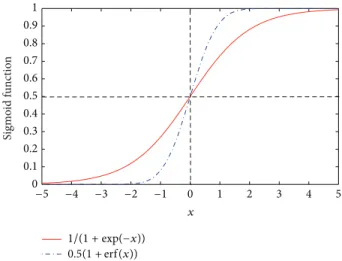
𝑑 𝑑𝑡erf(𝑡) = 2 √𝜋exp(−𝑡2) , for 𝑡 ∈R. (13) x Si gm o id fun ctio n 1 0.9 0.8 0.7 0.6 0.5 0.4 0.3 0.2 0.1 0 −5 −4 −3 −2 −1 0 1 2 3 4 5 1/(1 +exp(−x)) 0.5(1 +erf(x))

Figure 1: Sigmoid functions.

The good properties of the erf function are thus used to define a new sigmoid function, the sigmoid erf function:

sig(𝑥𝑖_𝑙) = 0.5 (1 +erf(𝑥𝑖_𝑙)) , (14)

which is a bounded differentiable real function defined for all 𝑥 ∈ R and has a positive derivative at each point. A comparison of both functions (9) and (14) is depicted in

Figure 1. Note that the slope at the origin of the sigmoid function in (14) is around 0.5641895, while that of function (9) is 0.25, thus yielding a faster growing from 0 to 1.

3.3. Rounding to Integer Part. The simplest discretization procedure of a continuous component of a point into 0/1 bit uses the rounding to the integer part function, known as floor function, and is described in [34]. Each continuous value

𝑥𝑖_𝑙 ∈ Ris transformed into a binary one, 0 bit or 1 bit,𝑏_𝑙𝑖,

for𝑙 = 1, . . . , 𝑛in the following way:

𝑏_𝑙𝑖_{= ⌊󵄨󵄨󵄨󵄨󵄨𝑥}𝑖_𝑙mod2󵄨󵄨󵄨󵄨󵄨⌋, (15)

where ⌊𝑧⌋ represents the floor function of𝑧 and gives the largest integer not greater than𝑧. The floating-point value

𝑥𝑖

𝑙 is first divided by 2 and then the absolute value of the

remainder is floored. The obtained integer number is the bit value of the component.

3.4. Heuristics Implementation. In this study, three methods capable of computing global solutions to binary optimization problems using FA are proposed.

3.4.1. Movement on Continuous Space. In this implemen-tation of the previously described heuristics, denoted by “movement on continuous space” (mCS), the movement of each firefly is made on the continuous space and its attractiveness term is updated considering the real position vector. The real position of firefly𝑖is discretized only after all movements towards brighter fireflies have been carried out. We note that the fitness evaluation of each firefly, for firefly

(5)

Discretize position of firefly𝑖:𝑥𝑖 → 𝑏𝑖,𝑖 = 1, . . . , 𝑚;

Compute𝑓(𝑏𝑖), 𝑖 = 1, . . . , 𝑚, rank fireflies (from lowest to largest𝑓); while 𝑘 ≤ 𝑘maxand󵄨󵄨󵄨󵄨𝑓(𝑏1) − 𝑓∗󵄨󵄨󵄨󵄨 > 𝜂do

forall𝑥𝑖such that𝑖 = 2, . . . , 𝑚do forall 𝑥𝑗such that𝑗 = 1, . . . , 𝑖 − 1do

Compute randomization term; Compute attractiveness𝛽;

Move position𝑥𝑖of firefly𝑖towards𝑥𝑗using (7); Discretize positions:𝑥𝑖 → 𝑏𝑖,𝑖 = 1, . . . , 𝑚;

Compute𝑓(𝑏𝑖), 𝑖 = 1, . . . , 𝑚, rank fireflies (from lowest to largest𝑓); Set𝑘 = 𝑘 + 1;

Algorithm 2: HBFA with mCS.

Compute𝑓(𝑏𝑖), 𝑖 = 1, . . . , 𝑚, rank fireflies (from lowest to largest𝑓); while𝑘 ≤ 𝑘maxand󵄨󵄨󵄨󵄨𝑓(𝑏1) − 𝑓∗󵄨󵄨󵄨󵄨 > 𝜂do

forall𝑏𝑖such that𝑖 = 2, . . . , 𝑚do forall𝑏𝑗such that𝑗 = 1, . . . , 𝑖 − 1do

Compute randomization term;

Compute attractiveness𝛽based on distance󵄩󵄩󵄩󵄩_󵄩𝑏𝑖− 𝑏𝑗󵄩󵄩󵄩󵄩_󵄩𝑝; Move binary position𝑏𝑖of firefly𝑖towards𝑏𝑗 using𝑥𝑖= 𝑏𝑖+ 𝛽(𝑏𝑗− 𝑏𝑖) + 𝛼𝐿(𝑏1)𝜎_𝑏𝑖; Discretize position of firefly𝑖:𝑥𝑖 → 𝑏𝑖;

Algorithm 3: HBFA with mBS.

ranking, is always based on the binary position.Algorithm 2

presents the main steps of HBFA with mCS.

3.4.2. Movement on Binary Space. This implementation, denoted by “movement on binary space” (mBS), moves the binary position of each firefly towards the binary positions of brighter fireflies; that is, each movement is made on the binary space although the corresponding position may fail to be 0 or 1 bit string and must be discretized before the updating of attractiveness. Here, fitness is also based on the binary positions.Algorithm 3presents the main steps of HBFA with mBS.

3.4.3. Probability for Binary Component. For this implemen-tation, named “probability for binary component” (pBC), we borrow the concept from the binary PSO [6, 9, 35] where each component of the velocity vector is directly used to compute the probability that the corresponding component of the particle position, 𝑥𝑖_𝑙, is 0 or 1. Similarly, in the FA algorithm, we do not interpret the vector𝑦𝑖in (7) as a step

size, but rather as a mean to compute the probability that each component of the position vector of firefly𝑖is 0 or 1. Thus, we define

𝑏_𝑙𝑖= {1, if rand≤sig(𝑦𝑙𝑖)

0, otherwise, (16) where sig()represents a sigmoid function.Algorithm 4is the pseudocode of HBFA with pBC.

4. Numerical Experiments

In this section, we present the computational results that were obtained with HBFA—Algorithms2,3, and4, using (9), (14), or (15)—aiming to investigate its performance when solving a set of binary nonlinear optimization problems. Two small 0-1 knapsack problems are also used to test the algorithms’ behavior on linear problems with 0/1 variables.

The numerical experiments were carried out on a PC Intel Core 2 Duo Processor E7500 with 2.9 GHz and 4 Gb of memory. The algorithms were coded in Matlab Version 8.0.0.783 (R2012b).

(6)

Compute𝑓(𝑏𝑖), 𝑖 = 1, . . . , 𝑚, rank fireflies (from lowest to largest𝑓); while𝑘 ≤ 𝑘maxand󵄨󵄨󵄨󵄨𝑓(𝑏1) − 𝑓∗󵄨󵄨󵄨󵄨 > 𝜂do

forall𝑏𝑖such that𝑖 = 2, . . . , 𝑚do forall𝑏𝑗such that𝑗 = 1, . . . , 𝑖 − 1do

Compute randomization term;

Compute attractiveness𝛽based on distance󵄩󵄩󵄩󵄩_󵄩𝑏𝑖− 𝑏𝑗󵄩󵄩󵄩󵄩_󵄩𝑝; Compute𝑦𝑖using binary positions (see (7));

Discretize𝑦𝑖and define𝑏𝑖using (16);

Algorithm 4: HBFA with pBC.

4.1. Experimental Setting. Each experiment was conducted 30 times. The size of the population is made to depend on the problem’s dimension and is set to𝑚 = min{40, 2𝑛}. Some experiments have been carried out to tune certain parameters of the algorithms. In the proposed FA with dynamic𝛼and𝛾, they are set as follows:𝛽₀ = 1,𝑝 = 1,𝛼_max = 0.5,𝛼_min =

0.01,𝛾_max = 10, and𝛾_min = 0.1. In Algorithms2(mCS),3

(mBS), and4(pBC), iterations were limited to𝑘_max = 500 and the tolerance for finding a good quality solution is𝜂 =

10−6. Results reported are averaged (over the 30 runs) of best function values, number of function evaluations, and number of iterations.

4.2. Experimental Results. First, we use a set of ten bench-mark nonlinear functions with different dimensions and characteristics. For example, five functions are unimodal and the remaining multimodal [3,9,10,36]. They are displayed

in Table 1. Although they are widely used in continuous

optimization, we now aim to converge to a 0/1 bit string solution.

First, we aim to compare with the results reported in [3, 9, 10]. Due to poor results, the authors in [10] do not recommend the use of ABC to solve binary-valued problems. The other metaheuristics therein implemented are the following:

(i) angle modulated PSO (AMPSO) and angle modu-lated DE (AMDE) that incorporate a trigonometric function as a bit string generator into the classic PSO and DE algorithms, respectively;

(ii) binary DE and PSO based on the sigmoid logistic function and (10), denoted by binDE and binPSO, respectively.

We noticed that the problems Foxholes, Griewank, Rosen-brock, Schaffer, and Step are not correctly described in [3,9,10]. Table 2 shows both the averaged best function values (obtained during the 30 runs),𝑓avg, with the St.D. in

parentheses, and the averaged number of function evalua-tions, nfe, obtained with the sigmoid logistic function (see in

(9)) and (10), while using the three implementations: mCS, mBS, and pBC. Results obtained for these ten functions indicate that our proposal HBFA produces high quality solutions and outperforms the binary versions binPSO and binDE, as well as AMPSO and AMDE. We also note that mCS has the best “nfe” values on 6 problems, mBS is better on 3 problems (one is a tie with mCS), and pBC on 2 problems. Thus, the performance of mCS is the best when compared with those of mBS and pBC. The latter is the least efficient of all, in particular for the large dimensional problems.

To analyze the statistical significance of the results we perform a Friedman test. This is a nonparametric statistical test to determine significant differences in mean for one independent variable with two or more levels—also denoted as treatments—and a dependent variable (or matched groups taken as the problems). The null hypothesis in this test is that the mean ranks assigned to the treatments under testing are the same. Since all three implementations are able to reach the solutions within the𝜂error tolerance on 9 out of 10 problems, the statistical analysis is based on the performance criterion “nfe.” In this hypothesis testing, we have three treatments and ten groups. Friedman’s chi-square has a value of 2.737 (with a𝑃value of 0.255). For 2 degrees of freedom reference

𝜒2 _{distribution, the critical value for a significance level of}

5% is 5.99. Hence, since 2.737≤ 5.99, the null hypothesis is not rejected and we conclude that there is no evidence that the three mean ranks values have statistically significant differences.

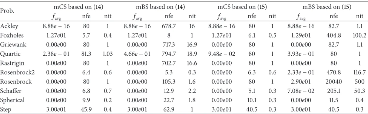
To further compare the sigmoid functions with the rounding to integer strategy, we include inTable 3the results obtained by the “erf” function in (14), together with (10), and the floor function in (15). Only the implementations mCS and mBS are tested. The table also shows the averaged number of iterations, nit. The results illustrate that implementation mCS (Algorithm 2) works very well with strategies based on (14), together with (10), and (15). The success rate for all the problems is 100%, meaning that the algorithms stop because the𝑓value at the position of the best/brightest firefly is within

(7)

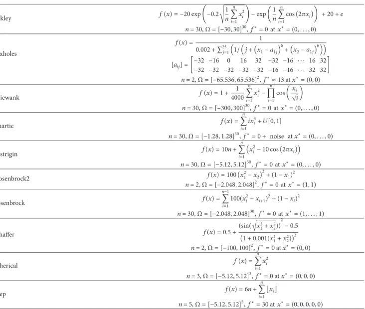
Table 1: Problems set. Ackley 𝑓 (𝑥) = −20exp(−0.2√ 1 𝑛 𝑛 ∑ 𝑖=1 𝑥2 𝑖) −exp(1_𝑛 𝑛 ∑ 𝑖=1 cos(2𝜋𝑥_𝑖)) + 20 + 𝑒 𝑛= 30,Ω = [−30, 30]30,𝑓∗= 0at𝑥∗= (0, . . . , 0) Foxholes 𝑓(𝑥) = 1 0.002 + ∑25_𝑗=1(1/ (𝑗 + (𝑥1− 𝑎1𝑗) 6 + (𝑥2− 𝑎2𝑗) 6 )) [𝑎𝑖𝑗] = [−32 −16 0_{−32 −32 −32 −32 −32 −16 −16 ⋅ ⋅ ⋅ 32 32}16 32 −32 −16 ⋅ ⋅ ⋅ 16 32] 𝑛= 2,Ω = [−65.536, 65.536]2,𝑓∗≈ 13at𝑥∗= (0, 0) Griewank 𝑓 (𝑥) = 1 + 1 4000 𝑛 ∑ 𝑖=1 𝑥2 𝑖 − 𝑛 ∏ 𝑖=1 cos(𝑥𝑖 √𝑖) 𝑛= 30,Ω = [−300, 300]30,𝑓∗= 0at𝑥∗= (0, . . . , 0) Quartic 𝑓(𝑥) = 𝑛 ∑ 𝑖=1 𝑖𝑥4 𝑖+ 𝑈[0, 1] 𝑛= 30,Ω = [−1.28, 1.28]30,𝑓∗= 0 + noise at𝑥∗= (0, . . . , 0) Rastrigin 𝑓(𝑥) = 10𝑛 + 𝑛 ∑ 𝑖=1 (𝑥2_𝑖− 10cos(2𝜋𝑥_𝑖)) 𝑛= 30,Ω = [−5.12, 5.12]30,𝑓∗= 0at𝑥∗= (0, . . . , 0) Rosenbrock2 𝑓(𝑥) = 100 (𝑥21− 𝑥2)2+ (1 − 𝑥1)2 𝑛= 2,Ω = [−2.048, 2.048]2,𝑓∗= 0at𝑥∗= (1, 1) Rosenbrock 𝑓(𝑥) = 𝑛−1 ∑ 𝑖=1 100(𝑥2 𝑖− 𝑥𝑖+1)2+ (1 − 𝑥𝑖)2 𝑛= 30,Ω = [−2.048, 2.048]30,𝑓∗= 0at𝑥∗= (1, . . . , 1) Schaffer 𝑓(𝑥) = 0.5 + (sin(√𝑥2₁+ 𝑥2₂))2− 0.5 (1 + 0.001(𝑥2 1+ 𝑥22))2 𝑛= 2,Ω = [−100, 100]2,𝑓∗= 0at𝑥∗= (0, 0) Spherical 𝑓 (𝑥) = 𝑛 ∑ 𝑖=1 𝑥2 𝑖 𝑛= 3,Ω = [−5.12, 5.12]3,𝑓∗= 0at𝑥∗= (0, 0, 0) Step 𝑓(𝑥) = 6𝑛 + 𝑛 ∑ 𝑖=1 ⌊𝑥𝑖⌋ 𝑛= 5,Ω = [−5.12, 5.12]5,𝑓∗= 30at𝑥∗= (0, 0, 0, 0, 0)

a tolerance𝜂of the optimal solution𝑓∗, in all runs. Further, mBS (Algorithm 3) works better when the discretization of the variables is carried out by (15). Overall, mCS based on (14) produces the best results on 6 problems, mCS based on (15) gives the best results on 7 problems (including 4 ties with the former case), mBS based on (14) wins only on one problem, and mBS based on (15) wins on 3 problems (all are ties with mCS based on (15)).

Further, when performing the Friedman test on the four distributions of “nfe” values, the chi-square statistical value is 13.747 (and the 𝑃 value is 0.0033). From the 𝜒2 distribution table, the critical value for a significance level of 5% and 3 degrees of freedom is 7.81. Since 13.747>7.81, the null hypothesis is rejected and we conclude that the observed differences of the four distributions are statistically significant.

We now introduce in the statistical analysis the results reported in Tables2and3concerned with both implementa-tions mCS and mBS. Six distribuimplementa-tions of “nfe” values are now

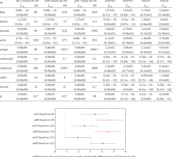
in comparison. Friedman’s chi-square value is 18.175 (𝑃value = 0.0027). The critical value of the chi-square distribution for a significance level of 5% and 5 degrees of freedom is 11.07. Thus, the null hypothesis of “no significant differences on mean ranks” is rejected and there is evidence that the six distributions of “nfe” values have statistically significant differences. Multiple comparisons (two at a time) may be carried out to determine which mean ranks are significantly different. The estimates of the 95% confidence intervals are shown in the graph of Figure 2 for each case under testing. Two compared distributions of “nfe” are significantly different if their intervals are disjoint and are not significantly different if their intervals overlap. Hence, from the six cases, we conclude that the mean ranks produced by mCS based on (15) are significantly different from those of mBS based on (9) and mBS based on (14). For the remaining pairs of comparison there are no significant differences on the mean ranks.

(8)

Table 2: Comparison with AMPSO, binPSO, binDE, and AMDE based on𝑓avgand St.D. (shown in parentheses).

Prob. mCS based on (9) mBS based on (9) pBC based on (9) AMPSO binPSO binDE AMDE

𝑓avg nfe 𝑓avg nfe 𝑓avg nfe 𝑓avg 𝑓avg 𝑓avg 𝑓avg

Ackley 8.88𝑒 − 16 80 8.88𝑒 − 16 1156 8.88𝑒 − 16 2168 1.97𝑒01 2.01𝑒01 1.73𝑒01 1.64𝑒01 (0.00𝑒00) (0.00𝑒00) (0.00𝑒00) (0.57𝑒 − 01) (0.49𝑒 − 01) (0.31𝑒01) (0.76𝑒00) Foxholes 1.27𝑒01 6.1 1.27𝑒01 7.2 1.27𝑒01 6.3 0.53𝑒 − 10 0.53𝑒 − 10 1.29𝑒01 5.0𝑒02 (9.03𝑒 − 15) (9.03𝑒 − 15) (9.03𝑒 − 15) (0.00𝑒00) (0.97𝑒 − 14) (0.86𝑒00) (0.0𝑒00) Griewank 0.00𝑒00 80 0.00𝑒00 1332 0.00𝑒00 2300 1.06𝑒02 6.79𝑒01 2.63𝑒02 2.06𝑒02 (0.00𝑒00) (0.00𝑒00) (0.00𝑒00) (0.44𝑒01) (0.98𝑒01) (0.10𝑒02) (0.39𝑒01) Quartic 4.55𝑒 − 01 2012 5.37𝑒 − 01 1771 4.88𝑒 − 01 2951 4.15𝑒01 2.09𝑒01 1.49𝑒00 3.55𝑒00 (3.01𝑒 − 01) (3.03𝑒 − 01) (2.71𝑒 − 01) (0.19𝑒01) (0.19𝑒01) (0.66𝑒00) (0.81𝑒00) Rastrigin 0.00𝑒00 80 0.00𝑒00 1282.7 0.00𝑒00 2406.7 2.25𝑒02 3.08𝑒02 2.14𝑒02 9.05𝑒01 (0.00𝑒00) (0.00𝑒00) (0.00𝑒00) (0.35𝑒02) (0.28𝑒01) (0.45𝑒02) (0.31𝑒02) Rosenbrock2 0.00𝑒00 6.5 0.00𝑒00 5.7 0.00𝑒00 6.1 0.49𝑒 − 04 0.14𝑒 − 03 0.20𝑒 − 05 0.55𝑒 − 04 (0.00𝑒00) (0.00𝑒00) (0.00𝑒00) (0.11𝑒 − 03) (0.88𝑒 − 04) (0.15𝑒 − 04) (0.17𝑒 − 04) Rosenbrock 0.00𝑒00 180 0.00𝑒00 2190.7 0.00𝑒00 2088 2.20𝑒03 2.24𝑒03 1.81𝑒03 9.14𝑒01 (0.00𝑒00) (0.00𝑒00) (0.00𝑒00) (0.86𝑒02) (0.77𝑒02) (0.16𝑒02) (0.42𝑒02) Schaffer 0.00𝑒00 6.1 0.00𝑒00 8 0.00𝑒00 4.9 0.24𝑒 − 01 0.73𝑒 − 01 −0.995𝑒00 −1.0𝑒00 (0.00𝑒00) (0.00𝑒00) (0.00𝑒00) (0.42𝑒 − 02) (0.11𝑒 − 01) (0.27𝑒 − 06) (0.0𝑒00) Spherical 0.00𝑒00 12 0.00𝑒00 12 0.00𝑒00 11.7 0.30𝑒 − 03 0.30𝑒 − 03 0.15𝑒 − 03 0.20𝑒 − 04 (0.00𝑒00) (0.00𝑒00) (0.00𝑒00) (0.00𝑒00) (0.0𝑒00) (0.41𝑒 − 04) (0.15𝑒 − 04) Step 3.00𝑒01 42.7 3.00𝑒01 42.7 3.00𝑒01 48 0.00𝑒00 0.17𝑒 − 04 0.15𝑒 − 01 0.25𝑒00 (0.00𝑒00) (0.00𝑒00) (0.00𝑒00) (0.00𝑒00) (0.15𝑒 − 04) (0.0𝑒00) (0.60𝑒 − 01) 0 1 2 3 4 5 6 mBS based on (15) mCS based on (15) mBS based on (14) mCS based on (₁₄) mBS based on (9) mCS based on (9)

mBS based on (9) and (14) have mean ranks significantly different from mCS based on (15) Figure 2: Confidence intervals for mean ranks of nfe.

For comparative purposes we include in Table 4 the results obtained by using the proposed L´evy (L) distribution in the randomization term, as shown in (7), and those pro-duced by the Uniform (U) distribution, using rand∼ 𝑈[0, 1] as shown in (3). The reported tests use implementation mCS (described inAlgorithm 2) with the two heuristics for binary variables: (i) the “erf” function in (14), together with (10), and (ii) the floor function in (15). It is shown that the performance of HBFA with Uniform distribution is very sensitive to the dimension of the problem, since the efficiency is good when

𝑛is small but gets worse when𝑛is large. Thus, we have shown that the L´evy distribution is a very good bid.

We add to some problems with𝑛 = 30fromTable 1— Ackley, Griewank, Rastrigin, Rosenbrock, and Spherical— three other functions Schwefel 2.22, Schwefel 2.26, and Sum of Different Power to compare our results with those reported in [1]. Schwefel 2.22 is unimodal and forΩ = [−10, 10]30, the binary solution is(0, . . . , 0)with𝑓∗ = 0; Schwefel 2.26 is multimodal and inΩ = [−500, 500]30, the binary solution

is(1, 1, . . . , 1)with𝑓∗ = −25.244129544; Sum of Different

Power is unimodal and inΩ = [−1, 1]30, the minimum is 0

at(0, . . . , 0). For the results ofTable 5, we use HBFA based

on mCS, with both “erf” function in (14), together with (10), and the floor function (15). The table reports on the average

(9)

Table 3: Comparison of mCS versus mBS and (14) versus (15), based on𝑓_avg, nfe, and nit.

Prob. mCS based on (14) mBS based on (14) mCS based on (15) mBS based on (15)

𝑓avg nfe nit 𝑓avg nfe nit 𝑓avg nfe nit 𝑓avg nfe nit

Ackley 8.88𝑒 − 16 80 1 8.88𝑒 − 16 678.7 16 8.88𝑒 − 16 80 1 8.88𝑒 − 16 82.7 1.1 Foxholes 1.27𝑒01 5.7 0.4 1.27𝑒01 8 1 1.27𝑒01 6.1 0.5 1.29𝑒01 404.8 100.2 Griewank 0.00𝑒00 80 1 0.00𝑒00 717.3 16.9 0.00𝑒00 80 1 0.00𝑒00 82.7 1.1 Quartic 2.38𝑒 − 01 81.3 1.03 4.66𝑒 − 01 794.7 18.9 9.48𝑒 − 02 80 1 3.93𝑒 − 01 80 1 Rastrigin 0.00𝑒00 80 1 0.00𝑒00 702.7 16.6 0.00𝑒00 80 1 0.00𝑒00 80 1 Rosenbrock2 0.00𝑒00 6.4 0.6 0.00𝑒00 5.3 0.3 0.00𝑒00 6.3 0.6 2.33𝑒 − 01 470.8 116.7 Rosenbrock 0.00𝑒00 80 1 0.00𝑒00 105.3 1.6 0.00𝑒00 80 1 2.90𝑒01 20040 500 Schaffer 0.00𝑒00 6.8 0.7 0.00𝑒00 12.9 2.2 0.00𝑒00 5.1 0.3 7.08𝑒 − 02 205.1 50.3 Spherical 0.00𝑒00 9.9 0.2 0.00𝑒00 22.7 1.8 0.00𝑒00 10.1 0.3 0.00𝑒00 11.5 0.4 Step 3.00𝑒01 45.9 0.4 3.00𝑒01 62.9 1 3.00𝑒01 40.5 0.3 3.00𝑒01 40.5 0.3

Table 4: Comparison between L´evy and Uniform distributions in the randomization term, based on𝑓avg, nfe, and nit (with St.D. in

parentheses).

Prob. mCS based on (14) + L mCS based on (14) + U mCS based on (15) + L mCS based on (15) + U

𝑓avg nfe nit 𝑓avg nfe nit 𝑓avg nfe nit 𝑓avg nfe nit

Ackley 8.88𝑒 − 16 80 1 8.88𝑒 − 16 1096 26.4 8.88𝑒 − 16 80 1 1.41e00 20040 500 (0.00𝑒00) (0.00𝑒00) (0.00𝑒00) (1.26𝑒 − 02) Foxholes 1.27𝑒01 5.7 0.4 1.27𝑒01 8 1 1.27𝑒01 6.1 0.5 1.27𝑒01 6.8 0.7 (9.03𝑒 − 15) (9.03𝑒 − 15) (9.03𝑒 − 15) (9.03𝑒 − 15) Griewank 0.00𝑒00 80 1 0.00𝑒00 2436 59.9 0.00𝑒00 80 1 1.27𝑒 − 01 20040 500 (0.00𝑒00) (0.00𝑒00) (0.00𝑒00) (2.76𝑒 − 02) Quartic 2.38𝑒 − 01 81.3 1.03 6.90𝑒00 14692 366.2 9.48𝑒 − 02 80 1 5.10𝑒 − 01 10581 263.5 (1.70𝑒 − 01) (1.16𝑒01) (1.03𝑒 − 01) (2.90𝑒 − 01) Rastrigin 0.00𝑒00 80 1 0.00𝑒00 1157 27.9 0.00𝑒00 80 1 1.00𝑒 − 01 18104 451.6 (0.00𝑒00) (0.00𝑒00) (0.00𝑒00) (4.03𝑒 − 01) Rosenbrock2 0.00𝑒00 6.4 0.6 0.00𝑒00 36.8 8.2 0.00𝑒00 6.3 0.6 0.00𝑒00 5.9 0.5 (0.00𝑒00) (0.00𝑒00) (0.00𝑒00) (0.00𝑒00) Rosenbrock 0.00𝑒00 80 1 8.22𝑒01 14136 352.4 0.00𝑒00 80 1 7.42𝑒01 17698 441.2 (0.00𝑒00) (1.02𝑒02) (0.00𝑒00) (8.43𝑒01) Schaffer 0.00𝑒00 6.8 0.7 0.00𝑒00 18.5 3.6 0.00𝑒00 5.1 0.3 0.00𝑒00 5.6 0.4 (0.00𝑒00) (0.00𝑒00) (0.00𝑒00) (0.00𝑒00) Spherical 0.00𝑒00 9.9 0.2 0.00𝑒00 13.3 0.7 0.00𝑒00 10.1 0.3 0.00𝑒00 14.7 0.8 (0.00𝑒00) (0.00𝑒00) (0.00𝑒00) (0.00𝑒00) Step 3.00𝑒01 45.9 0.4 3.00𝑒01 46.9 0.5 3.00𝑒01 40.5 0.3 3.00𝑒01 52.3 0.6 (0.00𝑒00) (0.00𝑒00) (0.00𝑒00) (0.00𝑒00)

Table 5: Comparison of HBFA (with mCS) with ABHS in [1] based on𝑓_avg, nfe, and SR (%).

Prob. mCS based on (14) mCS based on (15) ABHS in [1]

𝑓avg nfe SR (%) 𝑓avg nfe SR (%) 𝑓avg nfe SR (%)

Ackley 8.88𝑒 − 16 80 100 8.88𝑒 − 16 80 100 1.56𝑒 − 01 62350 90 Griewank 0.00𝑒00 80 100 0.00𝑒00 80 100 3.30𝑒 − 02 79758 38 Rastrigin 0.00𝑒00 80 100 0.00𝑒00 80 100 1.32𝑒01 90000 0 Rosenbrock 0.00𝑒00 80 100 0.00𝑒00 80 100 6.80𝑒02 90000 0 Schwefel 2.22 0.00𝑒00 80 100 0.00𝑒00 80 100 0.00𝑒00 59870 100 Schwefel 2.26 −2.52𝑒01 80 100 −2.47𝑒01 10867 87 −1.195𝑒04 90000 0 Spherical 0.00𝑒00 80 100 0.00𝑒00 80 100 0.00𝑒00 62234 100

(10)

Table 6: Results for varied dimensions (𝑛 = 50, 100, 200), considering𝑚 = 40.

𝑓∗ _𝑛 mCS based on (14) mCS based on (15)

𝑓avg St.D. nfe nit 𝑓avg St.D. nfe nit

Ackley 0.00𝑒00 50 8.88𝑒 − 16 0.00𝑒00 80 1 8.88𝑒 − 16 0.00𝑒00 80 1 0.00𝑒00 100 8.88𝑒 − 16 0.00𝑒00 80 1 8.88𝑒 − 16 0.00𝑒00 80 1 0.00𝑒00 200 8.88𝑒 − 16 0.00𝑒00 80 1 8.88𝑒 − 16 0.00𝑒00 80 1 Griewank 0.00𝑒00 50 0.00𝑒00 0.00𝑒00 80 1 0.00𝑒00 0.00𝑒00 80 1 0.00𝑒00 100 0.00𝑒00 0.00𝑒00 80 1 0.00𝑒00 0.00𝑒00 80 1 0.00𝑒00 200 0.00𝑒00 0.00𝑒00 80 1 0.00𝑒00 0.00𝑒00 80 1 Quartic 0.00𝑒00 +noise 50 2.24𝑒 − 01 1.95𝑒 − 01 82.7 1.1 1.43𝑒 − 01 1.59𝑒 − 01 80 1 0.00𝑒00 +noise 100 4.32𝑒 − 01 2.73𝑒 − 01 146.7 2.7 1.73𝑒 − 01 1.10𝑒 − 01 80 1 0.00𝑒00 +noise 200 5.23𝑒 − 01 2.94𝑒 − 01 1738.7 42.5 1.96𝑒 − 01 2.13𝑒 − 01 81.3 1.03 Rosenbrock 0.00𝑒00 50 0.00𝑒00 0.00𝑒00 80 1 0.00𝑒00 0.00𝑒00 80 1 0.00𝑒00 100 0.00𝑒00 0.00𝑒00 80 1 0.00𝑒00 0.00𝑒00 80 1 0.00𝑒00 200 0.00𝑒00 0.00𝑒00 80 1 0.00𝑒00 0.00𝑒00 80 1 Spherical 0.00𝑒00 50 0.00𝑒00 0.00𝑒00 80 1 0.00𝑒00 0.00𝑒00 80 1 0.00𝑒00 100 0.00𝑒00 0.00𝑒00 80 1 0.00𝑒00 0.00𝑒00 80 1 0.00𝑒00 200 0.00𝑒00 0.00𝑒00 80 1 0.00𝑒00 0.00𝑒00 80 1 Step 3.00𝑒02 50 3.00𝑒02 0.00𝑒00 80 1 3.00𝑒02 0.00𝑒00 80 1 6.00𝑒02 100 6.00𝑒02 0.00𝑒00 80 1 6.00𝑒02 0.00𝑒00 80 1 1.20𝑒03 200 1.20𝑒03 0.00𝑒00 80 1 1.20𝑒03 0.00𝑒00 80 1

function values, average number of function evaluations, and success rate (SR). Here, 50 independent runs were carried out to compare with the results shown in [1]. The maximum number of function evaluations therein used was 90000. It is shown that our HBFA outperforms the proposed adaptive binary harmony search (ABHS).

4.3. Effect of Problem’s Dimension on HBFA Performance. We now consider six problems with varied dimensions from the previous set to analyze the effect of problem’s dimension on the HBFA performance. We test three dimensions:𝑛 = 50,

𝑛 = 100, and 𝑛 = 200. The algorithm’s parameters are

set as previously defined. We remark that the size of the population for all the tested problems and dimensions is 40 points.

Table 6 contains the results for comparison based on

averaged values of 𝑓, number of function evaluations, and number of iterations. The “St.D.” of the 𝑓 values are also displayed. Since the implementation mCS, shown in

Algorithm 2, performs better and shows more consistent

results than the other two, we tested only mCS based on (14) and mCS based on (15).

Besides testing significant differences on the mean ranks produced by the two treatments, mCS based on (14) and mCS based on (15), we also want to determine if the differences on mean ranks produced by problem’s dimension—50, 100, and 200—are statistically significant at a significance level of 5%. Hence, we aim to analyze the effects of two factors “A” and “B.” “A” is the HBFA implementation (with two levels) and “B” is the problem’s dimension (with three levels). For this purpose, the results obtained for the six problems for each

combination of the levels of “A” and “B” are considered as replications. When performing the Friedman test for factor “A,” the chi-square statistical value is 1.225 (𝑃value = 0.2685) with 1 degree of freedom. The critical value for a significance level of 5% and 1 degree of freedom in the𝜒2 distribution table is 3.84, and there is no evidence of statistically significant differences. From the Friedman test for factor “B,” we also conclude that there is no evidence of statistically significant differences, since the chi-square statistical value is 0.746 (𝑃 value = 0.6886) with 2 degrees of freedom. (The critical value of the𝜒2distribution table for a significance level of 5% and 2 degrees of freedom is 5.99.) Hence, we conclude that the dimension of the problem does not affect the algorithm’s per-formance. Only with problem Quartic, the efficiency of mCS based on (14) gets worse as dimension increases. Overall, both tested strategies are rather effective when binary solutions are required on small as well as on large nonlinear optimization problems.

4.4. Solving 0-1 Knapsack Problems. Finally, we aim to analyze the behavior of our best tested strategies when solving well-known binary and linear optimization problems. For this preliminary experiment, we selected two small knap-sack problems. The 0-1 knapknap-sack problem (KP) can be described as follows. Let 𝑛be the number of items, from which we have to select some of them to be carried in a knapsack. Let 𝑤_𝑙 and V_𝑙 be the weight and the value of item 𝑙, respectively, and let 𝑊 be the knapsack’s capac-ity. It is usually assumed that all weights and values are nonnegative. The objective is to maximize the total value

(11)

of the knapsack under the constraint of the knapsack’s capacity: max_𝑥 𝑉 (𝑥) ≡ 𝑛 ∑ 𝑙=1 V_𝑙𝑥_𝑙 s.t. 𝑛 ∑ 𝑙=1 𝑤_𝑙𝑥_𝑙≤ 𝑊, 𝑥_𝑙∈ {0, 1} , 𝑙 = 1, . . . , 𝑛. (17)

If item𝑙is selected,𝑥_𝑙= 1; otherwise,𝑥_𝑙= 0. Using a penalty function, this problem can be transformed into

min_𝑥 − 𝑛 ∑ 𝑙=1 V_𝑙𝑥_𝑙+ 𝜇max{0, 𝑛 ∑ 𝑙=1 𝑤_𝑙𝑥_𝑙− 𝑊} , (18)

where𝜇is the penalty parameter which was set to be 100 in this experiment.

Case 1(an instance of a 0-1 KP with 4 items). Knapsack’s capacity is𝑊 = 6and the vectors of values and weights are

V= (40, 15, 20, 10)and𝑤 = (4, 2, 3, 1). Based on the

above-mentioned parameters, the HBFA with mCS based on (14) was run 30 times and the averaged results were the following. With a success rate of 100%, items 1 and 2 are included in the knapsack and items 3 and 4 are excluded, with a maximum value of 55 (St.D. = 0.0e00). On average, the runs required 0.8 iterations and 29.3 function evaluations. With a success rate of 23%, the heuristic based on the floor function, thus mCS based on (15), reached𝑓avg = 49(St.D. = 4.0e00) after

an average of 6161.1 function evaluations and an average of 384.1 iterations.

Case 2(an instance of a 0-1 KP with 8 items). The maximum capacity of the knapsack is set to 8 and the vectors of values and weights areV = (83, 14, 54, 79, 72, 52, 48, 62)and

𝑤 = (3, 2, 3, 2, 1, 2, 2, 3). The results are averaged over the 30

runs. After 8.7 iterations and 386.7 function evaluations, the maximum value produced by the strategy mCS based on (14) is 286 (St.D. = 0.0e00), with a success rate of 100%. Items 1, 4, 5, and 6 are included in the knapsack and the others are excluded. The heuristic mCS based on (15) did not reach the optimal solution. All runs required 500 iterations and 20040 function evaluations and the average function values were

𝑓avg= 227with St.D. = 3.14e01.

5. Conclusions and Future Work

In this work we have implemented several heuristics to compute a global optimal binary solution of bound con-strained nonlinear optimization problems, which have been incorporated into FA, yielding the herein called HBFA. The problems addressed in this study have bounded continu-ous search space. Our FA proposal uses dynamic updating schemes for two parameters,𝛾from the attractiveness term and𝛼from the randomization term, and considers the L´evy distribution to create randomness in firefly movement. The performance behavior of the proposed heuristics has been investigated. Three simple heuristics capable of transforming real continuous variables into binary ones are implemented.

A new sigmoid “erf” function is proposed. In the context of the firefly algorithm, three different implementations aiming to incorporate the heuristics for binary variables into FA are proposed (mCS, mBS, and pBC). Based on a set of benchmark problems, a comparison is carried out with other binary dealing metaheuristics, namely, AMPSO, binPSO, binDE, and AMDE. The experimental results show that the implementation denoted by mCS when combined with either the new sigmoid “erf” function or the rounding scheme based on the floor function is quite efficient and superior to the other methods in comparison. The statistical analysis carried out on the results shows evidence of statistically significant differences on efficiency, measured by the number of function evaluations, between the implementation mCS based on the floor function approach and the mBS based on both tested sigmoid functions schemes. We have also investigated the effect of problem’s dimension on the perfor-mance of our algorithm. Using the Friedman statistical test we conclude that the differences on efficiency are not statistically significant. Another simple experiment has shown that the implementation mCS with the sigmoid “erf” function is effective in solving two small 0-1 KP. The performance of this simple heuristic strategy will be further analyzed to solve large and multidimensional 0-1 KP. Future developments concerning the HBFA will consider its extension to deal with integer variables in nonlinear optimization problems. Different heuristics to transform continuous real variables into integer variables will be investigated. Challenging mixed-integer nonconvex nonlinear problems will be solved.

Conflict of Interests

The authors declare that there is no conflict of interests regarding the publication of this paper.

Acknowledgments

The authors wish to thank two anonymous referees for their valuable suggestions to improve the paper. This work has been supported by FCT (Fundação para a Ciência e Tecnologia, Portugal) in the scope of the Projects PEst-OE/MAT/UI0013/2014 and PEst-OE/EEI/UI0319/2014.

References

[1] L. Wang, R. Yang, Y. Xu, Q. Niu, P. M. Pardalos, and M. Fei, “An improved adaptive binary harmony search algorithm,” Information Sciences, vol. 232, pp. 58–87, 2013.

[2] M. A. K. Azad, A. M. A. C. Rocha, and E. M. G. P. Fernandes, “Improved binary artificial fish swarm algorithm for the 0-1 multidimensional knapsack problems,”Swarm and Evolution-ary Computation, vol. 14, pp. 66–75, 2014.

[3] A. P. Engelbrecht and G. Pampar´a, “Binary differential evolution strategies,” inProceedings of the IEEE Congress on Evolutionary Computation (CEC ’07), pp. 1942–1947, September 2007. [4] M. H. Kashan, N. Nahavandi, and A. H. Kashan, “DisABC: a

new artificial bee colony algorithm for binary optimization,” Applied Soft Computing Journal, vol. 12, no. 1, pp. 342–352, 2012.

(12)

[5] M. H. Kashan, A. H. Kashan, and N. Nahavandi, “A novel differential evolution algorithm for binary optimization,” Com-putational Optimization and Applications, vol. 55, no. 2, pp. 481– 513, 2013.

[6] J. Kennedy and R. C. Eberhart, “A discrete binary version of the particle swarm algorithm,” inProceedings of the IEEE International Conference on Systems, Man, and Cybernetics, vol. 5, pp. 4104–4108, Orlando, Fla, USA, October 1997.

[7] T. Liu, L. Zhang, and J. Zhang, “Study of binary artificial bee colony algorithm based on particle swarm optimization,” Journal of Computational Information Systems, vol. 9, no. 16, pp. 6459–6466, 2013.

[8] S. Mirjalili and A. Lewis, “S-shaped versus V-shaped transfer functions for binary particle swarm optimization,”Swarm and Evolutionary Computation, vol. 9, pp. 1–14, 2013.

[9] G. Pampar´a, A. P. Engelbrecht, and N. Franken, “Binary differential evolution,” inProceedings of the IEEE Congress on Evolutionary Computation (CEC ’06), pp. 1873–1879, Vancouver, Canada, July 2006.

[10] G. Pampar´a and A. P. Engelbrecht, “Binary artificial bee colony optimization,” inProceedings of the IEEE Symposium on Swarm Intelligence (SIS ’11), pp. 1–8, IEEE Perth, April 2011.

[11] S. Burer and A. N. Letchford, “Non-convex mixed-integer non-linear programming: a survey,”Surveys in Operations Research and Management Science, vol. 17, no. 2, pp. 97–106, 2012. [12] X.-S. Yang, “Firefly algorithms for multimodal optimization,”

inProceedings of the Stochastic Algorithms: Foundations and Applications (SAGA ’09), O. Watanabe and T. Zeugmann, Eds., vol. 5792 of Lecture Notes in Computer Science, pp. 169–178, 2009.

[13] X.-S. Yang, “Firefly algorithm, stochastic test functions and design optimization,”International Journal of Bio-Inspired Com-putation, vol. 2, no. 2, pp. 78–84, 2010.

[14] I. Fister Jr., X.-S. Yang, and J. Brest, “A comprehensive review of firefly algorithms,”Swarm and Evolutionary Computation, vol. 13, pp. 34–46, 2013.

[15] S. Yu, S. Yang, and S. Su, “Self-adaptive step firefly algorithm,” Journal of Applied Mathematics, vol. 2013, Article ID 832718, 8 pages, 2013.

[16] S. M. Farahani, A. A. Abshouri, B. Nasiri, and M. R. Meybodi, “A Gaussian firefly algorithm,”International Journal of Machine Learning and Computing, vol. 1, no. 5, pp. 448–453, 2011. [17] L. Guo, G.-G. Wang, H. Wang, and D. Wang, “An effective

hybrid firefly algorithm with harmony search for global numer-ical optimization,”The Scientific World Journal, vol. 2013, Article ID 125625, 9 pages, 2013.

[18] S. M. Farahani, A. A. Abshouri, B. Nasiri, and M. R. Meybodi, “Some hybrid models to improve firefly algorithm perfor-mance,”International Journal of Artificial Intelligence, vol. 8, no. 12, pp. 97–117, 2012.

[19] S. L. Tilahun and H. C. Ong, “Modified firefly algorithm,” Journal of Applied Mathematics, vol. 2012, Article ID 467631, 12 pages, 2012.

[20] X. Lin, Y. Zhong, and H. Zhang, “An enhanced firefly algorithm for function optimisation problems,”International Journal of Modelling, Identification and Control, vol. 18, no. 2, pp. 166–173, 2013.

[21] A. Manju and M. J. Nigam, “Firefly algorithm with fireflies having quantum behavior,” inProceedings of the International Conference on Radar, Communication and Computing (ICRCC ’12), pp. 117–119, IEEE, Tiruvannamalai, India, December 2012.

[22] X.-S. Yang and X. He, “Firefly algorithm: recent advances and applications,”International Journal of Swarm Intelligence, vol. 1, no. 1, pp. 36–50, 2013.

[23] S. Arora and S. Singh, “The firefly optimization algorithm: convergence analysis and parameter selection,” International Journal of Computer Applications, vol. 69, no. 3, pp. 48–52, 2013. [24] X.-S. Yang, S. S. S. Hosseini, and A. H. Gandomi, “Firefly algorithm for solving non-convex economic dispatch problems with valve loading effect,”Applied Soft Computing Journal, vol. 12, no. 3, pp. 1180–1186, 2012.

[25] A. H. Gandomi, X.-S. Yang, and A. H. Alavi, “Mixed variable structural optimization using firefly algorithm,”Computers and Structures, vol. 89, no. 23-24, pp. 2325–2336, 2011.

[26] X.-S. Yang, “Multiobjective firefly algorithm for continuous optimization,”Engineering with Computers, vol. 29, no. 2, pp. 175–184, 2013.

[27] A. N. Kumbharana and G. M. Pandey, “Solving travelling salesman problem using firefly algorithm,”International Journal for Research in Science & Advanced Technologies, vol. 2, no. 2, pp. 53–57, 2013.

[28] M. K. Sayadi, A. Hafezalkotob, and S. G. J. Naini, “Firefly-inspired algorithm for discrete optimization problems: an application to manufacturing cell formation,”Journal of Man-ufacturing Systems, vol. 32, no. 1, pp. 78–84, 2013.

[29] X.-S. Yang, “Firefly algorithm,” inNature-Inspired Metaheuristic Algorithms, pp. 81–96, Luniver Press, University of Cambridge, Cambridge, UK, 2nd edition, 2010.

[30] A. R. Jordehi and J. Jasni, “Parameter selection in particle swarm optimisation: a survey,”Journal of Experimental & Theoretical Artificial Intelligence, vol. 25, no. 4, pp. 527–542, 2013.

[31] M. Mahdavi, M. Fesanghary, and E. Damangir, “An improved harmony search algorithm for solving optimization problems,” Applied Mathematics and Computation, vol. 188, no. 2, pp. 1567– 1579, 2007.

[32] M. Padberg, “Harmony search algorithms for binary optimiza-tion problems,” inOperations Research Proceedings 2011, pp. 343–348, Springer, Berlin, Germany, 2012.

[33] M. A. K. Azad, A. M. A. C. Rocha, and E. M. G. P. Fernandes, “A simplified binary artificial fish swarm algorithm for unca-pacitated facility location problems,” inProceedings of World Congress on Engineering, S. I. Ao, L. Gelman, D. W. L. Hukins, A. Hunter, and A. M. Korsunsky, Eds., vol. 1, pp. 31–36, IAENG, London, UK, 2013.

[34] M. Sevkli and A. R. Guner, “A continuous particle swarm opti-mization algorithm for uncapacitated facility location problem,” inAnt Colony Optimization and Swarm Intelligence, M. Dorigo, L. M. Gambardella, M. Birattari, A. Martinoli, R. Poli, and T. St¨utzle, Eds., vol. 4150 ofLecture Notes in Computer Sciences, pp. 316–323, Springer, 2006.

[35] L. Wang and C. Singh, “Unit commitment considering genera-tor outages through a mixed-integer particle swarm optimiza-tion algorithm,”Applied Soft Computing Journal, vol. 9, no. 3, pp. 947–953, 2009.

[36] M. M. Ali, C. Khompatraporn, and Z. B. Zabinsky, “A numerical evaluation of several stochastic algorithms on selected con-tinuous global optimization test problems,”Journal of Global Optimization, vol. 31, no. 4, pp. 635–672, 2005.

(13)

Submit your manuscripts at

http://www.hindawi.com

Hindawi Publishing Corporation

http://www.hindawi.com Volume 2014

Mathematics

Journal of

Mathematical Problems in Engineering

Hindawi Publishing Corporation http://www.hindawi.com

Differential Equations

International Journal of

Volume 2014

Mathematical PhysicsAdvances in

Complex Analysis

Journal of

Optimization

Journal of

Combinatorics

International Journal of

Journal of

Function Spaces

Abstract and Applied Analysis

http://www.hindawi.com Volume 2014 International Journal of Mathematics and Mathematical Sciences

Hindawi Publishing Corporation http://www.hindawi.com Volume 2014

The Scientific

World Journal

Discrete Dynamics in Nature and Society

Discrete Mathematics

Journal of

http://www.hindawi.com Volume 2014 Hindawi Publishing Corporationhttp://www.hindawi.com Volume 2014

Research Article Heuristic-Based Firefly Algorithm for Bound Constrained Nonlinear Binary Optimization