Compressive Sequential Learning for Action Similarity Labeling

(1)

H

Compressive Sequential Learning for

Action Similarity Labeling

Jie Qin, Li Liu, Zhaoxiang Zhang,

Senior Member, IEEE

, Yunhong Wang,

Member, IEEE

,

and Ling Shao,

Senior Member, IEEE

Abstract— Human action recognition in videos has been

extensively studied in recent years due to its wide range of applications. Instead of classifying video sequences into a number of action categories, in this paper, we focus on a particular problem of action similarity labeling (ASLAN), which aims at verifying whether a pair of videos contain the same type of action or not. To address this challenge, a novel approach called compressive sequential learning (CSL) is proposed by leveraging the compressive sensing theory and sequential learning. We first project data points to a low-dimensional space by effectively exploring an important property in compressive sensing: the restricted isometry property. In particular, a very sparse measurement matrix is adopted to reduce the dimensionality efficiently. We then learn an ensemble classifier for measuring similarities between pairwise videos by iteratively minimizing its empirical risk with the AdaBoost strategy on the training set. Unlike conventional AdaBoost, the weak learner for each iteration is not explicitly defined and its parameters are learned through greedy optimization. Furthermore, an alternative of CSL named compressive sequential encoding is developed as an encoding technique and followed by a linear classifier to address the similarity-labeling problem. Our method has been systematically evaluated on four action data sets: ASLAN, KTH, HMDB51, and Hollywood2, and the results show the effectiveness and superiority of our method for ASLAN.

Index Terms— Action recognition, action similarity labeling,

pair matching, boosting, sparse random projection.

Manuscript received May 4, 2015; revised November 6, 2015; accepted December 8, 2015. Date of publication December 17, 2015; date of current version January 5, 2016. This work was supported in part by the Foundation for Innovative Research Groups through the National Natural Science Foun- dation of China under Grant 61573045 and Grant 61421003, in part by the Hong Kong, Macao and Taiwan Science and Technology Cooperation Program of China under Grant L2015TGA9004, in part by the National Natural Science Foundation of China under Grant 61528106, Grant 61375036, and Grant 61511130079, in part by the Newton International Exchanges Scheme, in part by the Program for New Century Excellent Talents in University, in part by the Beijing Higher Education Young Elite Teacher Project, and in part by the China Scholarship Council. The associate editor coordinating the review of this manuscript and approving it for publication was Prof. DimitriosTzovaras.

(Corresponding authors: Ling Shao and Yunhong Wang).

J. Qin and Y. Wang are with the Laboratory of Intelligent Recognition and Image Processing, State Key Laboratory of Virtual Reality Technology and Systems, School of Computer Science and Engineering, Beihang University, Beijing 100191, China (e-mail: [email protected]; [email protected]). L. Liu and L. Shao are with the Department of Computer Science and Digital Technologies, Northumbria University, Newcastle upon Tyne NE1 8ST, U.K. (e-mail: [email protected]; [email protected]).

Z. Zhang is with the Research Center for Brain-Inspired Intelligence, CAS Center for Excellence in Brain Science and Intelligence Technology, Institute of Automation, Chinese Academy of Sciences, Beijing 100190, China (e-mail: [email protected]).

I. INT RODUCT ION

UMAN action recognition in videos has been an active research area in computer vision spanning a wide range of application domains, such as intelligent surveillance, human-computer interaction, health monitoring and content- based video retrieval. Due to its vital importance, a variety of approaches have been proposed to address the problem of action classification or recognition [1]–[8]. The goal of human action recognition in videos is to classify unlabeled videos containing different types of actions into a predefined set of action categories. Recently, the computer vision com- munity has been mainly focusing on actions performed in unconstrained videos, targeting real-world action recognition. Unsurprisingly, these videos always present large variances in viewpoint, illumination, scale and appearance, and other complications such as occlusions, background cluttering and multiple actors performing actions in the same scene.

In such realistic settings, there is always an inevitable problem that different types of actions could exist in a short video sequence. It becomes extremely difficult to classify such a sequence into an exact type of action. For instance, a “springboard diving” mainly consists of “jumping”, “falling”, and “swimming”. How to define complex actions appropriately is highly subjective and may vary from one subject to another. In other words, class ambiguity is a common problem existing in multi-class action recognition, especially in unconstrained videos. Consequently, to avoid this ambiguity problem, action similarity labeling or action pair matching has been introduced by Kliper-Gross et al. [9] as another critical task, which is the focus of this paper, together with a benchmark dataset named The Action Similarity Labeling (ASLAN) Challenge (see Fig. 1 for examples of action pairs). The aim of action similarity labeling is to determine if the actors in two video sequences are performing the same action or not. In addition to avoiding the ambiguity of multi-class action recognition, action similarity labeling has its own advantages. Firstly, it is not limited to a given set of actions. In terms of multi-class action recognition, one may first learn the models corresponding to some predefined training actions and classify unknown videos based on these models. However, in the setting of action similarity labeling, no action labels are given. Therefore, it is a more generalized approach to determining whether two never-before-seen video sequences contain the same action. Secondly, action similarity labeling provides insights toward content-based video retrieval. Given an unknown video, retrieving videos

(2)

Fig. 1. Examples of (a) pairs of “same”-labeled actions and (b) pairs of “not-same”-labeled actions.

including the same type of action is the basic characteristic of image/video search engines. Thereby, addressing the similarity labeling/pair matching problem effectively and efficiently will enhance the performance of video retrieval significantly.

To address the action similarity labeling problem, several methods have been proposed [9]–[16], which can be mainly divided according to two perspectives: similarity measurement [9]–[13] and feature representation [14]–[16]. However, novel feature extraction and representation is a non-trivial task and learning a suitable metric or projection matrix to measure similarities of high dimensional vectors is typically complicated and time-consuming. In this work, we address the problem of action similarity labeling “in the wild” based on a novel approach called Compressive Sequential Learning (CSL), by exploring the techniques of compressive sensing and sequential learning. Due to complexities of realistic actions, high dimensional feature vectors are typically extracted, which usually leads to low computing efficiency and large storage space. To eliminate these shortcomings, we first project data points to a lower dimensional space based on an important property in compressive sensing: the Restricted Isometry Property (RIP) [17], which is able to preserve the distances between the points in a vector space. The projection can also obtain more compact data representations and balance the components’ variance [18]. Instead of the typical measurement matrix (random Gaussian matrix) satisfying RIP, we employ a very sparse random measurement matrix, which will reduce the memory and computational cost significantly. After projecting original high dimensional vectors to a relatively low dimensional space, a novel pair-wise sequential learning method motivated by [19] is proposed to exploit the information between pair-wise data based on the spirit of the boosting theory. In [19], a boosting strategy was utilized to learn each bit of an extremely compact binary local feature descriptor. However, in this work, by leveraging the boosting- trick, we simultaneously optimize the output of an ensemble classifier and reduce the empirical loss on pair-wise training data. Specifically, for each iteration of boosting, unlike [19], in which the weak learner is explicitly pre-defined, we learn a non-linear weak learner whose parameters are optimized based on the pair-wise training data and by efficiently using greedy optimization. The obtained CSL classifier is of the same form as a typical AdaBoost [20] strong classifier, being the sign of a linear combination of previously learned non-linear weak learners. Additionally, as an alternative to the sign function,

a linear SVM classifier is applied on the training data after aggregating the outputs of non-linear weak learners. In this case, our CSL method turns into Compressive Sequential Encoding (CSE), working as a strategy for extremely compact feature coding [21]–[23] for pair-wise data.

The rest of this paper is organized as follows. In Section II, related work for action similarity labeling is discussed. Section III describes our method in detail. The global sequential learning based on the boosting-trick is first proposed, and then the weak learner is defined and learned via greedy optimization. Subsequently, sparse random projection is introduced based on the compressive sensing theory. Finally, the overall framework is revisited and an alternative method to CSL is discussed. In Sections IV and V, extensive experimental results on four public action datasets, i.e., ASLAN, KTH, HMDB51 and Hollywood2, are shown, which prove the superiority of our method.

II. RELATED WORK

Action similarity labeling or action pair matching is a recently introduced task in the area of action recognition, focusing on the same/not-same classification of two never- before-seen video sequences. Performance in this task highly depends on the feature representation and the suitability of the similarity measurement used for comparing video pairs.

In terms of the similarity measurement, the first attempt [9] employed twelve pre-defined (dis-)similarity functions (e.g., Euclidean and chi-square distances) and their combinations as the baseline method. After that, Kliper-Gross et al. [11] proposed a supervised metric learning method called One Shot Similarity Metric Learning (OSSML) to learn a projection matrix which improves the (dis-)similarity between same/not-same training pairs in a reduced subspace of the original feature space. Moreover, before applying the final OSSML projection, PCA or Cosine Similarity Metric Learn- ing (CSML) was adopted as the initial projection. It has been validated on ASLAN that OSSML achieves better performance (approximately 4% improvement in terms of the Area Under Curve (AUC)) than manually defined (dis-)similarity functions. Similar to the metric learning method, Peng et al. [13] developed a large margin dimensionality reduction (LMDR) method to compress high-dimensional feature representations encoded by both Fisher Vector (FV) [24] and Vector of Locally Aggregated Descriptors (VLAD) [18]. A projection matrix was learned to increase the similarities of “same” video pairs and meanwhile separate “not-same” video pairs by a large margin. Instead of learning a proper metric, Cheng [10] proposed a similarity-score based paradigm to learn a rectangular similarity matrix of a fixed rank and applied it to pairwise-based action recognition. A Riemannian manifold-based optimization framework was exploited to learn the similarity matrix. Apart from learning a proper metric or a similarity matrix, the similarities of neighboring spatio-temporal points were explored in [12]. The space where the similarities lie in was discovered and mapped to another space with a fixed, smaller dimensionality. Thus, a novel similarity measurement between two image sequences was defined to form a similarity vector for further classification.

(3)

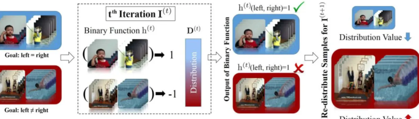
Fig. 2. The overall framework of Compressive Sequential Learning (CSL): Space-time features are first extracted from pair-wise action videos, followed by Bag-of-Features video representation. Two feature vectors extracted from a pair containing the same action are assigned label ‘+1’ and ‘−1’ means they belong to different action classes. Subsequently, sparse random projection is employed to project the high dimensional feature space to a lower one. Then our sequential learning is utilized to learn an optimized ensemble classifier, which can predict the labels for pair-wise data. Given a pair of testing videos, the learned classifier is applied to label the similarity of this pair.

As for the feature representation, most of the methods in the action similarity labeling task adopted those widely used in action recognition. For instance, the baseline results on ASLAN were obtained by leveraging Space-Time Interest Points (STIPs) followed by the Bag-of-Features (BoF) representation [25]. Kliper-Gross et al. [14] then proposed an enhanced feature encoding method named Motion Interchange Patterns (MIP) by capturing local changes in motion direc- tions. MIP was able to decouple image edges from the motion and compensate for global camera motion. Hanani et al. [15] explored new variants of the MIP framework by incorporating gradient-based descriptors and made the framework achieve a

in which only the pair labels are available during training rather than the individual label of each single data point.

A. Problem Formulation

Given a set of N training pairs of videos, {(v x _{i i}, v y )}, with Rm feature representation {(xi , yi )}, where xi and yi ∈ and

label {li } ∈ {+1, −1}, such that li = +1 if v x i iand v y contain

the same action, and li = −1 otherwise. We hope to find

a binary decision function (classifier) H(x, y) that is able to minimize the empirical loss on the training data:

N

better description of the motion’s structure. In particular, two variants histMIP and DoGMIP were proposed, which replaced

L =

i =1

(H(xi , yi ) = li ) (1)

the original patch representation by histogram of gradient orientations and Difference of Gaussians representations, respectively. These new variants were further combined with other features, such as STIPs [26], dense trajectories [27], [28] and Motion Boundary Histograms (MBH) [29], to achieve better performance. Inspired by a recently proposed tool in text processing named word2vec [30] neural network, a piggyback representation [16] was proposed to encode the local spatial arrangements of keypoints by employing a variant of the word2vec method.

III. ME T HODOL OGY

In this section, we will introduce our Compressive Sequen- tial Learning method in detail. The overall framework of CSL is shown in Fig. 2. The proposed method particularly aims at addressing the classification problem of pair-wise data,

Specifically, we adopt the boosting strategy similar to what is used in an AdaBoost classifier, aiming at iteratively learning the binary classifier to jointly minimize the empirical loss. Thus, the final classification function is the sign of a linear combination of non-linear weak learners:

T

H(x, y) = sign(

α(t )_h(t )_{(x, y)),}₍₂₎

t =1

where T is the number of iterations, α(t ) _{stands for the t-th}

vote corresponding to h(t ), and sign(x ) = +1 if x ≥ 0, and sign(x ) = −1 otherwise. α adjusts the classification result of pair-wise data in each iteration. In addition, h(x, y) is the weak learner whose definition and optimization will be introduced in Section III-C.

In the following sub-sections, we first introduce the boosting strategy for iteratively learning the final pair-wise

(4)

−

= + −

Fig. 3. The working flow of our sequential learning algorithm: In the t t h iteration, a binary function h(t ) (i.e., weak learner) is learned based on labeled pair-wise video samples and the current distribution over all the samples is updated as well. In the next iteration, if a video pair is misclassified by the weak learner, it will be assigned a larger distribution value, and vice versa. Hence, the following weak learner tends to correct the errors of the preceding ones. The final ensemble classifier is a linear combination of these weak learners.

ensemble classifier. Subsequently, how to formulate and optimize the non-linear weak learner is addressed. Finally, to reduce the computational cost, a sparse random projection method is proposed to further boost the performance.

B. Sequential Learning via Boosting

In this section, a boosting-based optimization method is adopted to iteratively minimize Eq. (1). The overall framework can been seen from Fig. 3. Boosting was first proposed in the computational learning theory literature [20], [31], [32] and has since received much attention. AdaBoost, also known as Adaptive Boosting, has been extensively studied and applied to many research areas. The goal of AdaBoost is to construct an ensemble classifier that minimizes the training error. The ensemble classifier consists of a number of weak classifiers, each of which can obtain a weak hypothesis whose training error is better than chance (i.e., less than 50%) on the training data, weighted by a distribution D. It is computationally infeasible to optimize the ensemble classifier to achieve the global minimal error on the training data. Therefore, a greedy optimization method is utilized to address this problem. The vote α corresponding to the weak learner and distribution D

that weights the training data are updated iteratively to ensure the overall decrease of the training error for the ensemble classifier. Specifically, in each iteration, α is computed according to the weighted training error, and D is updated so that the pair-wise data points that are misclassified by the previous iteration are assigned a higher weight, whereas those points that are correctly classified are assigned a lower weight.

During the last few decades, a variety of AdaBoost variants have been proposed, including Discrete AdaBoost, Real AdaBoost [33], LogitBoost and Gentle AdaBoost [34]. In practice, we follow the spirit of Gentle AdaBoost and

Meanwhile, due to the different rule of updating the vote α, Gentle AdaBoost is proved to be more efficient than the traditional AdaBoost.

C. Optimized Weak Learner

Unlike other weak learners used in the boosting strategy, our weak learner should be able to address the classification problem of pair-wise data. In the pair-wise setting, only the label of each pair is available instead of the label of any single data point. The weak learner h(x, y) adopted in the boosting algorithm should be capable of predicting whether two data points belong to the same class or not. Thereby, the objective of this weak learner is to minimize the least-squares loss on the training data:

N

min (h(xi , yi ) − li )2 . (3) i =1

Intuitively, we define the weak learner as a product of two sign functions as follows:

h(x, y) = sign(wT x + b) sign(wT y + b), (4) where the function inside the sign has a standard form of a linear function with w and b as its parameters.

Particularly, by applying the weak learner of this form, the predictions of labels for pair-wise data will be +1 if two data points belong to the same class, and −1 otherwise. In the following, we will learn the parameters w and b via greedy optimization. Note that N min (h(xi , yi ) li )2 w,b i =1 N

adopt it to optimize the global objective function in Eq. (1). = min

(h(xi , yi )2 + l 2 i i i

Gentle AdaBoost is different from the widely used traditional AdaBoost with regard to how they use the weighted training

w,b i =1

N i − 2l h(x , y ))

error to update the vote α. Empirical evidence indicates that Gentle AdaBoost has similar or superior performance to the traditional AdaBoost on regular data, but presents its advantage on noisy data and is much more resistant to outliers.

min

(1 1 2li h(xi , yi )). (5) w,b

i =1

The weak learner h(x, y) that minimizes Eq. (5) is also the one that maximizes the correlation of its output and the

(5)

= + + → i = i = eeding data labels. Based on this fact, parameters w and b can be

optimized by: N max li h(xi , yi ) w,b i =1 N max li sign(wT xi b)sign(wT yi b) w,b i =1 N = max li sign( )sign( ), (6) w

i =1 wT xi wT yi _{Fig. 4. Sparse Random Projection:}_P_{is the sparse random measurement}

where w w by simply adding b behind the last entry of w matrix. Each row of P contains β non-zero entries (the white grids represent zero entries). By applying P on the original high-dimensional data x , a more and xi →

of xi or yi .

yi by adding 1 behind the last entry _compact_x _i

can be obtained with a low computational cost (i.e., totally kβ

Since the sign function in the weak learner is non- differentiable, Eq. (6) is still hard to solve. Here, the spectral relaxation trick [35], [36] is applied and the sign function is approximated by using its signed magnitude, i.e., sign(x ) = x . Therefore, by dropping the sign function, Eq. (6) can be relaxed as:

N

multiplications, where k , β ± m).

video sequences containing actions “in the wild” (computing

ws and bs requires eigen decompositions of (m +1)×(m +1)

matrices). In this sub-section, we focus on projecting the pair-wise data from the high dimensional space to a suitable low one. In particular, we adopt the spirit of sparse random max

li ( )( ) projection. Fig. 4 shows our sparse random projection method,

w

i =1 _wT _x

i N

wT yi which has the following advantages: (1) simultaneously pre-

serving the structure of the original high dimensional space;

= max

li (2) obtaining compact low-dimensional feature representa-w

i =1

wT xi yi T w N

tions; (3) balancing the components’ variance of the original feature vector. In the following, we will first introduce random

wT xi yi T )w. (7) projection and further propose our sparse random projection

max

w (

i =1

li

method.

Moreover, w in Eq. (7) can be optimized by solving: Given a set of data points {xi }N ₁, where xi ∈ Rm , our goal

is to find a random matrix P ∈ Rk×m , which projects xi to xi

where Z = N

max

w

li xi yi T .

wT Zw, (8)

in a much lower dimensional space R_{up the computation:} k (k ± m) for sp

i =1

It is worth in Eq. (8) turns into a standard eigen x Px . (9)

not g that w can _i= _i

decomposition problem. Hence, the optimal solution for

be obtained in a closed-form as the eigenvector of Z associated According to the Johnson-Lindenstrauss (JL) lemma [37], distances between the points in a vector space are very likely with the largest eigenvalue. Additionally, since yi _{preserved if they are projected onto a randomly selected}

xi and

are equivalent to each other (i.e., h(xi , yi ) = h(yi , xi )),

Z can be transformed into its symmetric form such that

subspace with suitably high dimensions. Furthermore, as [38]

Z = N li (xi yi T +yi xi T ) before solving w, which simplifies proves, the random matrix satisfying the JL lemma also holds

the

i =1 _{for the Restricted Isometry Property in compressive sensing.}

calculation.

Although the optimization is not global, it yields a practical approximation to the optimal solution to Eq. (6). Furthermore,

owing to the iterative optimization of the global boosting strategy, a series of sub-optimal weak learners can also achieve promising classification performance after several iterations.

(6)

as Additionally, due to the simplification of our weak learner,

computational costs in each iteration can be significantly reduced.

D. Sparse Random Projection

In the above sub-sections, a global and local optimization framework for dealing with the classification of pair-wise data has been proposed. Although the computational complexity can be reduced to a certain extent, it is still high due to the high dimensionality of complex features extracted from

Therefore, if the random matrix P satisfies the JL lemma, P is able to preserve the structure of the high dimensional space, namely the distances between all pairs of original data points. In other words, if xi is compressive, such as audio or image

data, it can be reconstructed with a minimum error from xi

with high probability. In addition to structure-preserving, mentioned in [18], P can balance the components’ variance of xi after performing the projection, which will directly

benefit the optimization of weak learners.

In terms of conventional random projections [39], the entries of the measurement matrix P (denoted by { pi j }) should be i.i.d.

with a zero mean. A convenient way is to let pi j follow a sym-

metric distribution about zero with a unit variance. Therefore, a typical measurement matrix P is drawn from a Gaussian ensemble randomly with pi j ∼ N (0, 1). In this case, P is a

(7)

√

m

10

⎪

Algorithm 1 Compressive Sequential Learning

a non-trivial task in many practical computational environments. To address this problem, Achlioptas [37] proposed sparse random projections using the measurement matrix P

with i.i.d. entries in

Finally, we obtain a linear combination of non-linear optimized weak learners. By simply feeding to the sign function, an ensemble classifier is learned to measure similarities between pair-wise data points. Meanwhile, before applying the sign

⎧ _{1 function, we obtain the confidence values and treat them as}

⎪1, wi t h pr obabi li t y 2s ⎪ ⎨ 1 pi j = s 0, wi t h pr obabi li t y 1 − (10)

one dimensional feature vectors for pairs of data. And a linear SVM classifier is trained on these 1D vectors from the training

s set and then applied to predict labels for testing pairs of data.

⎪

1

In this way, our CSL can be seen as an encoding technique

⎩−1, wi t h pr obabi li t y

2s

where s = 1 or s = 3. In this case, the random measurement matrix P becomes very sparse and is very easy to compute. By setting s = 3, a three-fold speedup can be guaranteed since only one third of the data need to be computed. Furthermore, in [39], Li et al. showed that even larger values of s could be employed, such as s = √m, with little loss in accuracy. If s = √m, a √m-fold speedup can be achieved. In particular, we utilize a coefficient ξ ∈ ( 1 , 0.1] to set s and control the sparsity of the random projection matrix: s = m × ξ . When

ξ = 0.1, the random projection matrix P could be extremely sparse, i.e., a m -fold speedup can be achieved. However, in practice, s should not be set too aggressively to retain robustness.

E. Compressive Sequential Learning and Encoding

As aforementioned, our method incorporates the spirits of compressive sensing and sequential learning, and the focus of our method is classification of pair-wise data. Therefore, we name it Compressive Sequential Learning. The overall framework is outlined in Fig. 2, and the figure inside the dashed box is the core process of our CSL method. Furthermore, Algorithm 1 illustrates the detailed procedure of our method. It can be seen from Fig. 2 and Algorithm 1 that the boosting- trick is utilized as the global optimization technique. In each iteration, sparse random projection is first employed to reduce the dimensionality of the original feature space. Based on the low dimensional feature vectors from the training set, our weak learner is optimized by solving Eq. (8). After finding

the optimized weak learner, we follow the formulation in Algorithm 1 to obtain and update the distribution D and vote α.

(8)

for embedding pair-wise data to extremely compact codes, i.e., one dimensional feature vectors. This method, named Compressive Sequential Encoding (CSE), can be seen as an alternative to the CSL classifier. Both CSL and CSE are extensively evaluated in Section V.

F. Complexity Analysis

As illustrated in Algorithm 1, the cost of our CSL algorithm mainly consists of three parts within the “for” loop. The first part is for the construction of sparse random projection matrices. From Section III-D, we can conclude that its time complexity is O (km), where m is the dimensionality of the original space and k is that of the projected low-dimensional space. The second part is for the multiplications of projection matrices and N data points xi ∈ Rm . The time complexity

of the matrix multiplication is O (km N ). The last part is for the optimization of weak learners as shown in Eq. (8), which is a standard eigen-decomposition problem. Therefore, the time complexity of the last part is O (k3 ₎_{. In total, the time} complexity of our CSL algorithm is O (T × (km + km N + k3₎₎_, where T is the number of iterations of the global boosting framework. Furthermore, since k ± m, the computational complexity of our method is equivalent to O (T km N ).

In addition, we analyze the computational complexities of the state-of-the-art methods for action similarity learning [11], [13]–[15], which are shown in Table I. The complexity of OSSML [11] mainly consists of two parts, i.e., computing gradient of its objective function, and using cross validation to estimate the optimal values of its parameters. Specifically, the complexity of OSSML is O (T km2 Nbc), where T is the number of iterations used to optimize the projection

(9)

Fig. 5. Example frames of actions in the four datasets, i.e., ASLAN, KTH, HMDB51 and Hollywood2. TABLE I

COMP U TAT I ONAL CO M P L E X IT IE S O F DIFFE R E N T METHODS . T , T

AND T DENOT E NUMBERS OF ITER AT I ONS OF DI FFE R E N T OP T IM IZ AT I ON ALGORI T HMS US E D B Y DIFFE R E N T METHODS . PL EAS E SEE T EXT F OR MORE DE TAI LS

matrix, b is the number of values of the parameter tested in the cross validation process, c is the number of steps in the gradient descent method. Both [14] and [15] mainly focus on the feature representation problem and employ the metric learning method named CSML [40] for similarity learning, whose complexity is similar to that of OSSML. Specifically, the complexities of [14] and [15] are both

O (T km N bc). Obviously, our CSL method is much more efficient than [11], [14], and [15]. In terms of LMDR [13], its complexity is mainly due to the quadratic optimization about the projection matrix, which is addressed by the stochastic sub-gradient descent method. Thus, the overall cost of LMDR is O (T km N ), where T denotes the number of iterations of the stochastic sub-gradient descent method. As shown in [13], LMDR needs 10k iterations (i.e., T = 10,000) to achieve the optimal results, while only 50 iterations (i.e., T = 50) are enough for our method to achieve comparable results as discussed in Section V-D. Therefore, our method also needs less computational complexity than LMDR.

IV. DATASE T S AND EXPERIMENTAL SETUP

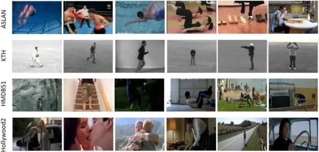
To evaluate our approach, extensive experiments are conducted on a variety of action datasets, especially on challenging action datasets containing videos “in the wild”. Specifically, four public datasets for action recognition (i.e., ASLAN, KTH, HMDB51 and Hollywood2) are used in our experiments. Fig. 5 illustrates some example frames of the action sequences in the datasets. From the figure,

we can see that actions in ASLAN, HMDB51 and Hollywood2 are of extremely high complexity. The video sequences usually contain large variations in camera motion, scale, view, background, illumination, etc. Additionally, we evaluate our method on KTH, which contains videos under constrained environments. We conduct experiments on both constrained and realistic action datasets to illustrate the challenge posed when using videos “in the wild” compared to laboratory produced videos. In the following sub-sections, we describe each of the four datasets briefly. Since we focus on the problem of similarity labeling, the protocol for creating video pairs is also explained. Subsequently, spatial-temporal feature extraction and video representation methods are presented in detail, as well as the overall experimental protocol.

A. Datasets

1) ASLAN: The Action Similarity Labeling (ASLAN) Challenge is a recent dataset, which contains 3,631 action videos collected from the web with over 400 complex action classes. The goal of this dataset is to decide if two videos present the same action or not, following training with “same” and “not-same”-labeled video pairs. We follow the test protocol used in [9], in which the action pairs for training and test are mutually exclusive, i.e., actions in the test set are neither available during training nor from any action classes in the training set. In short, this protocol is known as the unseen pair matching. Specifically, ASLAN includes two views, one view (View-1) for model selection and algorithm develop- ment, and the other one (View-2) for reporting performance. We demonstrate the performance of our method on View-2, which consists of 10 mutually exclusive subsets. Each subset contains 600 action video pairs: 300 same and 300 not-same.

2) KTH: KTH [41] is an early action dataset acquired in a controlled environment. It contains six types of human actions, e.g., walking and jogging. Each action is performed several times by 25 subjects in four conditions. All action

(10)

μ SE

m

sequences were taken over homogeneous backgrounds with a static camera with a 25fps frame rate. To validate our method in terms of unseen pair matching, we follow the setting in [9]. Specifically, six actions in KTH are divided into three mutually exclusive subsets.

3) HMDB51: HMDB51 [42] is known as a large video database for human motion recognition, containing 6849 video clips collected from various sources such as movies and YouTube. There are totally 51 action categories, each of which includes at least 101 video sequences. In our experiments, we use a subset of HMDB51, which consists of 2963 clips belonging to 19 action categories of general body movements. In order to create action pairs, we randomly choose five mutually exclusive subsets on the 19 action classes. Similar to the ASLAN dataset, each subset contains 600 action video pairs: 300 same and 300 not-same. Note that we use the original videos rather than the stabilized ones in our experiments.

4) Hollywood2: The Hollywood2 [43] dataset is composed of 1707 action samples with 12 action classes. All the videos are extracted from 69 different Hollywood movies.

STIP descriptors randomly selected from the training data, and Euclidean distance is used to calculate the distances between STIP descriptors and 5000 visual words.

C. Experimental Protocol

In terms of reporting performance, we follow the testing protocol used in [9]. The final results are reported in an N-fold leave-one-out cross-validation scheme on the aforementioned four datasets. In each experiment, N−1 of the subsets are used for training, with the rest one used for testing. This results in N separate classification problems and the final performance is reported using the mean accuracy (see Eq. (11)) and the standard error of the mean (see Eq. (12)) over the N subsets. Meanwhile, the ROC curve is constructed and the Area Under the Curve (AUC) is calculated for classifiers used on the N test subsets.

N

Pn

μ = n=1 _,₍₁₁₎

N

The dataset intends to provide a comprehensive benchmark for human action recognition in realistic and challenging settings.

where Pn is the classification accuracy using subset n for

testing.

To create action pairs, we randomly divide 823 training _σ N

μ)2 σ n=1 ( Pn −

samples into three mutually exclusive subsets, each of which contains 300 same action video pairs and 300 not-same ones.

SE = √

N, = N − 1 (12)

B. Space-Time Video Representation

We use the same features employed in [9] to produce baseline results on the ASLAN dataset, which are sparse

We do individual experiments using each of the three features as well as the combination of these features. Additionally, to allow for efficient computation, PCA is employed to project the high dimensional feature vectors to a reduced dimensional space before applying our method (the value of

m is space-time features first proposed in [26]. These features can

provide tolerance to clutter, occlusions and scale changes. Specifically, Space-Time Interest Points are detected using a space-time extension of the Harris operator and three types of local descriptors are computed to represent local motion and appearance features, i.e., Histogram of Oriented Gradients (HOG), Histogram of Optical Flow (HOF), and a composition of these two referred to as HNF. These local feature descriptors are computed for 3D video patches in the neighborhood of detected STIPs. Each video patch is divided into a grid with 3×3×2 blocks. Then 4-bin HOG, 5-bin HOF, and 8-bin HNF descriptors are computed for each block. By concatenating the blocks, each detected STIP is referred to as a 72-element, 90-element or 144-element descriptor.

To represent a video sequence containing a set of such descriptors, we adopt the widely used spatial-temporal Bag-of-Features (BoF) model. A visual vocabulary is assem- bled by clustering all the descriptors of training videos. Each STIP of the video sequence is assigned a label corresponding to its closest visual word of the vocabulary. Therefore, a video sequence is the composite of a set of visual words. The frequency of occurrences of each word belonging to the video sequence is calculated and normalized into a histogram, which is the final BoF representation. In our experiments, one visual vocabulary is needed for each of our N experiments (N=10, 3, 5 and 3 for ASLAN, KTH, HMDB51 and Hollywood2, respectively). For each experiment, k-means

(11)

dimensions). After that, sparse random projection is applied to further reduce the dimension and boost the performance. Due to the randomness of our sparse projection, each experiment is performed 200 times and the final results reported are averaged from the 200 runs.

V. EXPERIMENTAL RE SULT S A. Comparison With Baselines

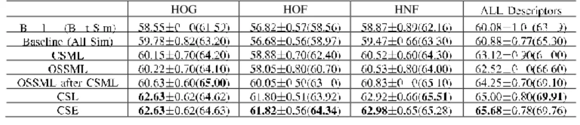
We first apply our CSL method on the four datasets and compare our results with the baseline results in terms of the accuracy, standard error and AUC (see Tables II-V for details). Specifically, the baseline method in [9] calculates 12 distances/similarities between feature vectors of the benchmark pairs. The specific formulations of these similarity functions can be seen from [9]. Due to space limitation, we manually select the best performance of these similarity functions and show the best results among them, which correspond to rows of “Baseline (Best Sim)” in the tables. Furthermore, the values of the 12 (dis-)similarities are concatenated into vectors and a linear SVM classifier is trained on the 12D vectors of pairs of action samples from the training set. As shown in [9], the combination of 12 similarity functions can often achieve the best classification results. Therefore, we compare the performance of our CSL method with the best results of the 12 similarities, as well as the concatenated results corresponding to rows of “Baseline (All Sim)” in the tables.

(12)

TABLE II

CLAS S I FIC ATI ON PERF O RMANCE O N ASL AN: ACCUR ACY ± STANDAR D E RROR AND (AUC) (%),

AVERAGED OVER T HE 10-FOLD S . PLEAS E SEE T EXT F OR MORE DETA I LS

TABLE III

CLAS S I FIC ATI ON PERF O RMANCE O N KT H: ACCUR ACY ± STANDARD E RROR AND (AUC) (%),

AVERAGED OVER T HE 3-FOLDS . PL EAS E SEE T EXT F OR MORE DE TAI L S

TABLE IV

CLAS S I FIC ATI ON PERF O RMANCE O N HMDB51: ACCURACY ± STANDARD E RROR AND (AUC) (%),

TABLE V

CLAS S I FIC ATI ON PERF O RMANCE O N HOLLY WOOD 2: ACCUR ACY ± STANDAR D E RROR AND (AUC) (%),

As aforementioned in Section III, apart from our CSL method, we obtain the confidence values before applying the sign function in Eq. (2), which are 1D feature vectors for pairs of samples. Then a binary, linear SVM classifier is trained on these vectors and their corresponding binary labels to map unknown pairs to a binary decision of same/not-same. These results are shown on the last row of each table corresponding to “CSE”.

In order to acquire the fusion results of the aforementioned three features, i.e., HOG, HOF and HNF, two strategies are employed. In terms of our CSL method, the weighted voting strategy is adopted. In particular, the final fused prediction of our CSL classifier is the sign of summation of confidence outputs of three individual CSL classifiers applied on these three features. As for the fusion results of the baseline and CSE, we follow [9] and utilize the stacking technique [44]. Specifically, the (dis-)similarity values of all three features (w.r.t. baseline) or the confidence outputs of CSL (w.r.t. CSE) are concatenated to form three dimensional vectors, each of which represents a pair of example videos. A linear SVM classifier is then trained

on these vectors with their corresponding same or not-same labels. All the fusion results are shown in the last columns of the tables.

As shown in Tables II-V, we can conclude that, for either using CSL as a classification method or an encoding method, it can always outperform the manually-defined similarity functions and their combinations. In comparison of the best classification results between the baseline and our methods, a 4.80%, 9.44%, 2.40% or 3.22% improvement can be guaranteed on ASLAN, KTH, HMDB51 and Hollywood2, respectively. For the most challenging datasets, such as ASLAN and HMDB51, applying a linear SVM classifier on the confidence outputs of CSL can achieve slightly better performance. In most cases, the standard errors of our methods are lower than those of the baseline, showing the generalization of our classification method on different subsets. It is noteworthy that our method can achieve a significant improvement over the baseline on the KTH dataset, especially when using HOG and HOF features. This demonstrates the capability of our method on action similarity labeling under constrained environments.

(13)

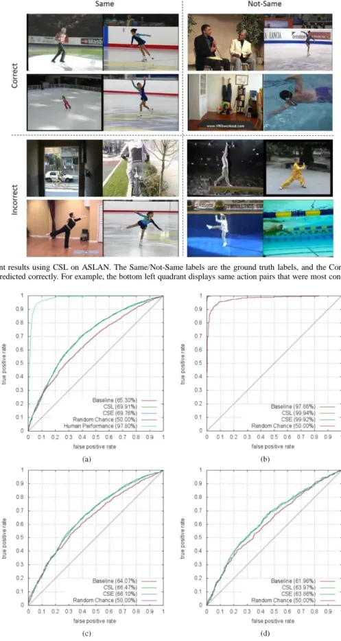
Fig. 6. The most confident results using CSL on ASLAN. The Same/Not-Same labels are the ground truth labels, and the Correct/Incorrect labels indicate whether our CSL method predicted correctly. For example, the bottom left quadrant displays same action pairs that were most confidently labeled as not-same.

Fig. 7. ROC curves of different methods evaluated on the (a) ASLAN, (b) KTH, (c) HMDB51 and (d) Hollywood2 datasets. In addition to demonstrating the accuracies, standard

errors and AUC, ROC curves of the classification results of different approaches are shown in Fig. 7. The ROC

curves are constructed based on the results of N classification experiments. As specified in Section IV-C, in each experiment, N−1 subsets are used for learning our CSL classifier and we

(14)

evaluate the results on the rest of the set. For each dataset, an ROC curve is constructed for all of its subsets together. In other words, the confidence output for each testing pair is computed in each experiment and all the outputs for N testing sets are concatenated together.

To gain further insight into our experimental results, we illustrate the most confident predictions on the ASLAN dataset made by our CSL method. Here, the level of confidence is measured by the value before applying the sign function in Eq. (2), i.e., the highest values correspond to the most confident predictions. Fig. 6 presents the most confident correct same and not-same predictions, and the most confident incorrect same and not-same ones. These images demonstrate the challenges and complexities of action similarity labeling in realistic scenes. Many of the mistakes result from misleading context. For instance, same action pairs are misclassified because of pose ambiguity and viewpoint variance. Meanwhile, not-same action pairs are mistaken as same ones due to a similar background and camera motion.

B. Comparison With State-of-the-Art

Since the ASLAN dataset has been collected as a benchmark focusing on the similarity labeling challenge, we further compare our method with the state-of-the-art methods.

Firstly, we evaluate our method in terms of similarity learning by comparing with the state-of-the-art metric learning methods (i.e., CSML and OSSML). The 3rd to 5th rows of Table II show the results of CSML, OSSML and “OSSML after CSML” which are taken from [11]. Initial PCA projection was done before applying the OSSML and CSML, and “OSSML after CSML” means applying the OSSML method with the matrix obtained by using the CSML algorithm as the initial projection. Obviously, “OSSML after CSML” can always achieve the best performance in comparison with its counterparts, i.e., CSML and OSSML. Specifically, our method achieves a 2.00%, 1.77%, 2.15% or 1.43% improvement over “OSSML after CSML” in accuracy with regard to different features and their combinations, respectively. Therefore, from the table, we can conclude that our learning algorithm is well suited for measuring the similarities between pairs of videos, even better than some state-of-the-art metric learning algorithms. Moreover, by applying very sparse random projection, our optimization algorithm is solved in the very low (less than 50) dimensional space, which can reduce the computational complexity significantly.

Secondly, for fairly comparing the performance of our method with the state-of-the-art methods on the ASLAN benchmark, we follow [13] and extract improved dense trajectories (IDT) with HOG, HOF and MBH concatenated 396-element descriptors using the code from Wang and Schmid [45]. After feature extraction, VLAD [18] is employed for video representation and its codebook size is fixed to 256 as commonly used in the literature [45]. Fig. 8 shows the comparison results with the state-of-the-art methods. Apart from [13], both our CSL and CSE methods outperform other state-of-the-art methods. The accuracy of our method is 0.57% less than that of [13]. It should be

Fig. 8. Comparison with the state-of-the-art methods on the ASLAN benchmark.

Fig. 9. Total errors on the training data of the ASLAN dataset using different feature descriptors.

noted that [13] utilized a dimensionality reduction method to compress high-dimensional feature vectors and their best results were obtained by using 59% compression ratio, which reduced the original dimensionality to 874. However, as aforementioned, our method is performed on feature vectors with less than 50 dimensions. Therefore, the very little loss in accuracy is acceptable with large enhancement in computational efficiency.

C. Training Error of CSL

Since the boosting strategy is employed in our sequential learning process, the total error on the training data should be evaluated. In particular, we demonstrate the classification error on the ASLAN dataset by using different feature representations, i.e., HOG, HOF and HNF. As aforementioned, there are totally 10 experiments. A training error illustrated in Fig. 9 is averaged over training errors calculated from each of the 10 training sets. As shown in Fig. 9, although there exist several rising points, the overall total error on the training data decreases gradually with the increase of the number of iterations. This downward trend indicates the effectiveness of our boosting-based sequential learning algorithm. As the number of iterations increases, we can learn a pair-wise classification model that minimizes the error on the training sets step by step. Owing to this fact, we are able to label the similarity between pairs of testing examples effectively.

(15)

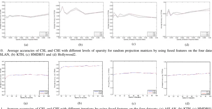
Fig. 10. Average accuracies of CSL and CSE with different levels of sparsity for random projection matrices by using fused features on the four datasets: (a) ASLAN, (b) KTH, (c) HMDB51 and (d) Hollywood2.

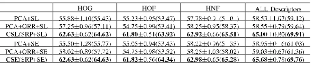
Fig. 11. Average accuracies of CSL and CSE with different iterations by using fused features on the four datasets: (a) ASLAN, (b) KTH, (c) HMDB51 and (d) Hollywood2.

D. Evaluation of Parameters

To further study the influence of several parameters on the performance of CSL and CSE, we evaluate our methods based on different settings of parameters, i.e., number of iterations w.r.t boosting and sparsity of the random projection matrix. Firstly, as shown in Fig. 10, we demonstrate the performance by using different levels of sparsity ξ for random projection matrices. Fig. 10 shows the average accuracies using the combination of three feature descriptors on all the four datasets, respectively. As shown in Fig. 10, there is less than 2% difference between a lowest average accuracy and a highest one on all the four datasets. Therefore, we can conclude that the sparseness of the random projection matrix has little influence on the final performance. Particularly, we can employ a very sparse measurement matrix to project the high dimensional data, which will result in a significant speedup in computational efficiency. Secondly, the performance of our method is illustrated with the increasing iterations of the boosting process. From Fig. 11, we can see that only five iterations can already achieve acceptable performance. In most cases, more iterations usually guarantee a higher accuracy. Specifically, the performance grows rapidly when the number of iterations increases to 20, especially on the ASLAN and KTH datasets. In addition, there is little variation in terms of the accuracy after 50 iterations on most datasets. Although more iterations will result in higher accuracies, this will in turn cost more computing time. Therefore, in our experiments, we set the number of iterations as 50 to ensure a good balance between the performance and the computational efficiency.

E. Evaluation of the Overall Framework

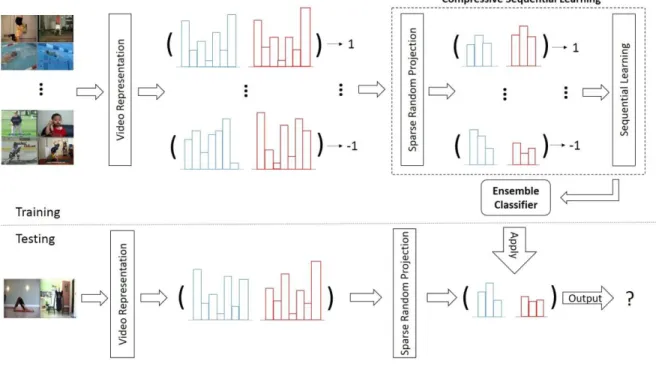
As our framework consists of two major steps: dimensionality reduction via sparse random projection and sequential learning/encoding via boosting, we further validate the choices for each step by replacing our method with several other

methods in each step. Firstly, for dimensionality reduction, we utilize two methods, i.e., PCA and PCA with orthogonal random rotation (ORR) as suggested by Jégou et al. [18], instead of our sparse random projection (SRP). The original feature space is reduced to 50 dimensions after applying these two methods. Then we utilize our sequential learning (SL) or sequential encoding (SE) method based on the low dimensional space. Note that our sequential learning (SL) or encoding (SE) method can be seen as an alternative to each other. If we apply the sign function, our method can be seen as a classification method specifically developed for pair-wise data, otherwise our method can be regarded as a compact encoding method. Therefore, for fairly validating the choice for the second step, we first reduce the original dimension using our SRP method and conduct the experiments from two perspectives. Firstly, we replace our choice for this step with several other classification methods, i.e., Gentle AdaBoost [34], Real AdaBoost [33], SVM [46] and K Nearest Neighbours (KNN), for comparisons with our CSL method. Secondly, we utilize Gentle AdaBoost and Real AdaBoost as encoding methods by discarding the sign function, followed by a linear SVM classifier for the final classification, and this is comparable to our CSE method.

When validating the choice for the second step, our pair- wise sequential learning/encoding method is substituted by other methods, so we need to represent the similarity between a pair of video clips. Here, we follow [14] and [15] and transform representations of each pair, i.e., xi and yi to a single

vector by performing point-wise multiplications of the two vectors (xi . ∗ yi , where .∗ denotes point-wise multiplication).

All the results by using different features are demonstrated in Table VI and VII, and the last column shows the fusion results based on the aforementioned weighted voting or stacking technique [44]. It can be seen that, our choices (i.e., SRP, SL and SE) consistently outperform different choices of other

(16)

TABLE VI

E VA L UAT I O N O F T H E FI R S T STEP (i.e., DI M ENS I ONALI T Y REDUCT I ON ) OF OUR OVERALL FR AME WO RK ON THE ASL AN BENCHMARK : ACCURACY ± STANDAR D E RROR AND (AUC) (%), AVERAGED OVER T HE 10-FOLD S . PLEA S E SEE T EXT F OR MORE DE TAI LS

TABLE VII

E VA L UAT I O N O F T H E SECOND STEP (i.e., SEQUENT I A L L EARNI N G /E NC O DI N G ) OF OUR OVERALL FRAME WO RK ON THE ASL AN BENCHMARK : ACCURACY ± STANDAR D E RROR AND (AUC) (%), AVERAGED OVER T HE 10-FOLD S . PLEA S E SEE T EXT F OR MORE DE TAI LS

methods for different steps, which proves the superiority of our overall framework.

VI. CONCL USION

In this paper, we consider the action similarity labeling challenge in realistic scenarios. A novel method named Compressive Sequential Learning (CSL) has been presented for learning the similarities between pairs of actions. A very sparse random projection based on the Restricted Isometry Property in the compressive sensing theory is employed for projecting data points to a low dimensional vector space, where the distances between the points are preserved. We then address the similarity measurement as a greedy optimization problem, by incorporating a boosting trick globally and optimizing non-linear weak classifiers for pair-wise data locally. Our method has been systematically evaluated on the ASLAN, KTH, HMDB51 and Hollywood2 action datasets. The results demonstrate the superiority of our method over other state-of-the-art methods. For future work, we plan to further improve the optimization algorithm, e.g., to employ more sophisticated weak learners, and investigate its applications to other related areas.

REFE RE NCE S

[1] I. Everts, J. C. van Gemert, and T. Gevers, “Evaluation of color spatiotemporal interest points for human action recognition,” IEEE Trans. Image Process., vol. 23, no. 4, pp. 1569–1580, Apr. 2014.

[2] M. Yu, L. Liu, and L. Shao, “Structure-preserving binary representations for RGB-D action recognition,” IEEE Trans. Pattern Anal. Mach. Intell., doi: 10.1109/TPAMI.2015.2491925.

[3] K. Guo, P. Ishwar, and J. Konrad, “Action recognition from video using feature covariance matrices,” IEEE Trans. Image Process., vol. 22, no. 6, pp. 2479–2494, Jun. 2013.

[4] F. Zhu and L. Shao, “Weakly-supervised cross-domain dictionary learning for visual recognition,” Int. J. Comput. Vis., vol. 109, nos. 1–2, pp. 42–59, Aug. 2014.

[5] A. Oikonomopoulos, I. Patras, and M. Pantic, “Spatiotemporal local- ization and categorization of human actions in unsegmented image sequences,” IEEE Trans. Image Process., vol. 20, no. 4, pp. 1126–1140, Apr. 2011.

[6] L. Shao, L. Liu, and M. Yu, “Kernelized multiview projection for robust action recognition,” Int. J. Comput. Vis., 2015, doi: 10.1007/s11263-015- 0861-6.

[7] L. Liu, L. Shao, X. Li, and K. Lu, “Learning spatio-temporal representations for action recognition: A genetic programming approach,” IEEE Trans. Cybern., doi: 10.1109/TCYB.2015.2399172.

[8] L. Shao, X. Zhen, D. Tao, and X. Li, “Spatio-temporal Laplacian pyramid coding for action recognition,” IEEE Trans. Cybern., vol. 44, no. 6, pp. 817–827, Jun. 2014.

[9] O. Kliper-Gross, T. Hassner, and L. Wolf, “The action similarity labeling challenge,” IEEE Trans. Pattern Anal. Mach. Intell., vol. 34, no. 3, pp. 615–621, Mar. 2012.

[10] L. Cheng, “Riemannian similarity learning,” in Proc. 30th Int. Conf. Mach. Learn., vol. 28. 2013, pp. 540–548.

[11] O. Kliper-Gross, T. Hassner, and L. Wolf, “One shot similarity metric learning for action recognition,” in Proc. 1st Int. Conf. Similarity-Based Pattern Recognit., 2011, pp. 31–45.

[12] I. Kotsia and I. Patras, “Exploring the similarities of neighboring spatiotemporal points for action pair matching,” in Proc. 11th Asian Conf. Comput. Vis., 2013, pp. 624–635.

[13] X. Peng, Y. Qiao, Q. Peng, and Q. Wang, “Large margin dimensionality reduction for action similarity labeling,” IEEE Signal Process. Lett., vol. 21, no. 8, pp. 1022–1025, Aug. 2014.

[14] O. Kliper-Gross, Y. Gurovich, T. Hassner, and L. Wolf, “Motion interchange patterns for action recognition in unconstrained videos,” in Proc. 12th Eur. Conf. Comput. Vis., 2012, pp. 256–269.

[15] Y. Hanani, N. Levy, and L. Wolf, “Evaluating new variants of motion interchange patterns,” in Proc. IEEE Conf. Comput. Vis. Pattern Recognit. Workshops (CVPRW), Jun. 2013, pp. 263–268.

[16] L. Wolf, Y. Hanani, and T. Hassner, “A piggyback representation for action recognition,” in Proc. IEEE Conf. Comput. Vis. Pattern Recognit. Workshops (CVPRW), Jun. 2014, pp. 520–525.

[17] E. J. Candès and T. Tao, “Decoding by linear programming,” IEEE Trans. Inf. Theory, vol. 51, no. 12, pp. 4203–4215, Dec. 2005. [18] H. Jégou, M. Douze, C. Schmid, and P. Perez, “Aggregating local

descriptors into a compact image representation,” in Proc. IEEE Conf. Comput. Vis. Pattern Recognit. (CVPR), Jun. 2010, pp. 3304–3311. [19] T. Trzcinski, M. Christoudias, P. Fua, and V. Lepetit, “Boosting

binary keypoint descriptors,” in Proc. IEEE Conf. Comput. Vis. Pattern Recognit., Jun. 2013, pp. 2874–2881.