DOI 10.1007/s11721-017-0145-6
PolyACO+: a multi-level polygon-based ant colony
optimisation classifier
Morten Goodwin1 · Torry Tufteland1 ·
Guro Ødesneltvedt1 · Anis Yazidi2
Received: 30 September 2016 / Accepted: 4 November 2017 / Published online: 16 November 2017 © Springer Science+Business Media, LLC, part of Springer Nature 2017
Abstract Ant colony optimisation (ACO) for classification has mostly been limited to rule-based approaches where artificial ants walk on datasets in order to extract rules from the trends in the data, and hybrid approaches which attempt to boost the performance of existing classifiers through guided feature reductions or parameter optimisations. A recent notable example that is distinct from the mainstream approaches is PolyACO, which is a proof-of-concept polygon-based classifier that resorts to ACO as a technique to create multi-edged polygons as class separators. Despite possessing some promise, PolyACO has some sig-nificant limitations, most notably, the fact of supporting classification of only two classes, including two features per class. This paper introduces PolyACO+, which is an extension of PolyACO in three significant ways: (1) PolyACO+ supports classifying multiple classes, (2) PolyACO+ supports polygons in multiple dimensions enabling classification with more than two features, and (3) PolyACO+ substantially reduces the training time compared to Poly-ACO by using the concept of multi-levelling. This paper empirically demonstrates that these updates improve the algorithm to such a degree that it becomes comparable to state-of-the-art techniques such as SVM, neural networks, and AntMiner+.
Keywords Ant colony optimisation·Classification·Polygon·Multi-levelling
A preliminary version of this paper (Goodwin and Yazidi2016) can be found in the Proceedings of the 10th International Conference on Swarm Intelligence, ANTS 2016. Part of this work has also been published as a Master’s Thesis at University of Agder, Norway, Spring of 2016.
B
Anis Yazidi [email protected]1 Department of Computer Science, University of Agder, Grimstad, Norway
2 Department of Computer Science, Oslo and Akershus University College of Applied Sciences, Oslo,
1 Introduction
Classification is the problem of predicting categories of unknown items on the basis of training data, and it is very common in machine learning with important application areas. Some well-known examples include predicting sentiments of sentences, pinpointing objects in images, detecting patient deaths, and predicting the best move in Go. Hundreds of papers are published on the topic each year, which has resulted in a myriad of classification algorithms differing in principle, implementation, and performance. Classification becomes intrinsically challenging whenever the data to be classified are not easily separable in the feature space (Caruana et al.2008; Madjarov et al.2012).
Some of the best known classification techniques, such as support vector machine (SVM) and perceptron-based classifiers, rely upon constructing mathematical functions having weights that efficiently separate two or more classes of data in the feature space. In two-dimensional spaces, the separation boundary might be nonlinear and thus the decision boundaries might be complex. SVM deals with this situation by either projecting the data on a higher-dimensional space or using a “kernel trick”, which provides a separator not limited to a linear or polynomial function. The adoption of a kernel is equivalent to transposing the data to many dimensions, but the accuracy depends on the right choice of the kernel functions as well as on several other parameters. The latter choice is usually performed through manual trial and error.
The training process of a classifier can be considered as an optimisation task, and ant colony optimisation (ACO) specifically has been proposed for training classifiers in three general areas. Firstly, ACO is commonly applied as a method to enhance state-of-the-art classifiers through parameter optimisations (Daly and Shen2009; Sharma et al.2012; Abadeh et al.
2008; De Campos and Puerta2008; Daly et al.2011; Jun-Zhong et al.2009). Secondly, some prominent studies, including AntMiner and AntMiner+, have used ACO as a rule-based classifier (Martens et al.2007). Thirdly, some recent advances have introduced PolyACO, a polygon-based classification algorithm (Goodwin and Yazidi2016; Tufteland et al.2016).1 Interestingly, PolyACO deals with the classification problem in a completely different manner from existing classifiers. Instead of relying upon mathematical functions, PolyACO surrounds the classes with polygons guided by artificial ants and ray casting.
This paper introduces PolyACO+, an extension of the existing PolyACO algorithm. Poly-ACO+ includes two main enhancements. Firstly, it is extended through its ability to classify multiple classes. PolyACO applies one polygon per problem, whereas PolyACO+ applies one polygon per class. This approach is similar to how an SVM deals with multiple classes. Secondly, PolyACO+ can handle datasets with more than two features. Since most datasets have multiple features, this enhancement makes PolyACO+ more suitable for real classifica-tion problems. This is achieved by taking majority votes on multiple two-feature projecclassifica-tions, i.e. by invoking PolyACO+ on various 2-D spaces. The number of planes forndimensions is calculated by counting the combinations of dimension pairs using the binomial coefficient:
n
2
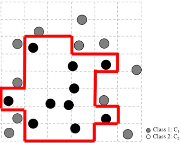
. The ants walk along several two-dimensional planes, and in each plane the ants construct a polygon per class. Figure1shows a polygon constructed by PolyACO+ for the classC1
in a two-dimensional plane. Furthermore, for performance reasons, the PolyACO+ reward function is designed to support a parallel architecture optimised to run on GPUs. These improvements make PolyACO+ dramatically faster and more accurate than its predecessor. Empirical results show that PolyACO+ performs similarly or better than other state-of-the-art classification algorithms in several classification tasks in terms of classification accuracy.
Fig. 1 Example of a simple two-class classification scenario with the classes black (C1) and
grey (C2), each with two features
Class 1: C1
Class 2: C2
Nevertheless, despite PolyACO+’s very good performance, its major hurdle is the rather long training time.
As for other classifiers, PolyACO+ has a training phase and a classification phase. The former’s aim is to create polygons that encircle classes of items so that the polygons separate the training classes from each other. In this phase PolyACO+ finds a polygonsj∗per class
Cjper pair of dimensions, consisting of vertices and edges. PolyACO+ maximises a function that measures how well the polygonsjseparates the items of classCjfrom the others during the training phase. Thus, formally speaking, we aim to find ansj∗ ∈Sso thatf(sj∗)≥ f(sj) for each classCj per pair of dimensions, whereSconsists of all possible polygons and the function f(sj)measures how well polygonsjseparates the data . The aim in the classification phase is to use the polygons as a basis to determine to which class a new unknown item to be classified belongs. The classification determines whether the item to be classified is within or outside of the polygons, for each dimension. The overall classification result is a combination of classifications in all dimensions.
The paper is organised as follows. Section2presents the state of the art in ACO-based classification. Section3introduces PolyACO+. Section4presents the results from applying PolyACO+ to classification problems and compares the results with state-of-the-art classi-fiers. Finally, Sect.5concludes and presents further work to be completed in this field.
2 State of the art
In order to place the work into the correct context, this section presents different state-of-the-art algorithms for classification, placing an emphasis on classification using ACO.
2.1 Rule discovery classification
Rule discovery is a data mining task that generates a set of rules describing each class or category in a dataset. Based on labelled data, the algorithm defines a set of rules. The goal is to make predictions about unknown data using IF<conditions>THEN<class>rules, where<conditions>is constructed by terms in the form of (term1 AND term2 AND…).
From a historical perspective, the first application that used ACO for classification was AntMiner (Parpinelli et al.2002). AntMiner is an algorithm that uses artificial ants to discover
classification rules. Several improvements to AntMiner have been suggested through the years (Liu et al.2003), of which one very successful example is AntMiner+ (Martens et al.2007). AntMiner+ is an extension of AntMiner, which includes modifications such as a directed acyclic graph to create the environment on which the ants move (Martens et al.2007,2011). It also usesMAX–MIN ant system (MMAS) (Stützle and Hoos2000) to manage ant behaviour and pheromones and has anearly stoppingcriterion (discussed further below).
AntMiner+ starts by creating a directed acyclic graph environment. An ant starts in the
Startvertex and stops at theStopvertex. The resulting path represents a potential rule. The paths that are walked by most ants, according to a predetermined threshold, are kept as classification rules. Similar toMMAS, only the ants that achieve the globally highest score update the pheromones, and all values are adjusted to stay within the boundariesτmaxand τmin. The algorithm converges when one path reachesτmaxand all others are equal toτmin.
Subsequently, the rule associated with the path containingτmaxis extracted along with the
training data covered by it. Ants are continuously released until a stop condition is reached. This can either be an early stopping criterion or the fact that none of the ants is able to extract a rule that covers at least one training point. If the latter happens, no rule can be extracted as all the paths have zero quality. This is typically caused by noise in the remaining data, which indicates that further rule induction is useless.
In contrast, AntMiner+ resorts to early stopping to avoid over-fitting. An early stop happens when the error measure on the validation set (one set which is 1/3 of the training set) starts to increase. Training is then stopped, thus effectively preventing the rule from fitting the training data noise. It should be noted that early stopping causes loss of data that cannot be used for construction rules and is therefore better fitted for larger datasets.
In addition to the previously mentioned AntMiner series including its variations (Martens et al. 2007, 2011; Tripathy et al. 2013; Aribarg et al. 2012), the literature also includes other ACO rule-based classifiers. Perhaps the most notable example is Ant-labeler, a semi-supervised method for assigning labels to unlabelled data (Albinati et al.2015). It uses ACO as a learning method and, during a self-training process, generates rule-based models. This results in a pheromone matrix from which classification rules are derived.
2.2 PolyACO
PolyACO is a grid-based polygon algorithm aimed at creating boundaries by surrounding and separating classes guided by ACO (Goodwin and Yazidi2016; Tufteland et al.2016). Figure2presents an overview included here for explanatory purposes. The figure is an excerpt from the original PolyACO paper (Goodwin and Yazidi2016) and shows an example of how PolyACO is trained for the two classesC1andC2by surrounding items from onlyC1with
a polygon. A similar approach has been proposed using learning automata in Goodwin et al. (2016).
PolyACO is a rudimentary classification algorithm that only supports classification of two classes at once and only classes that have two features. The reason for this is that in PolyACO the ants explore solutions in a grid-like graph environment that is generated from the training data. Therefore, PolyACO is limited to solving classification problems in two-dimensional spaces.
Ants are released sequentially with random initial positions. The ants explore and find paths in a similar manner to traditional ACO for path finding. Instead of finding a path from a source to a goal, they end up at the same position from which they started. When ants return to their original position, their travelled path will have formed a polygon shape. To determine path quality, PolyACO uses a combination of the polygon perimeter and a score of how well
Training Classification
ACO Ray tracing
Labeled data Polygon
Unknown items to be labeled Class 1: C1
Class 2: C2
Fig. 2 Overview of training and classification in PolyACO. In the training phase, ACO is used to create a polygon that separates the classes, and items are classified based on whether they are inside or outside of the polygon. Classification happens through ray tracing where geometric rays are cast at they-value of items to determine if the polygon surrounds the items
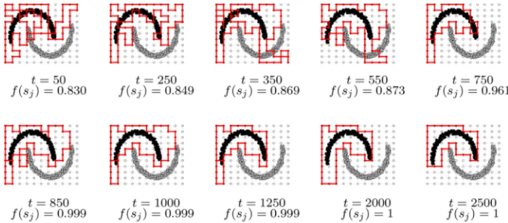
Fig. 3 Example of best known polygonsj∗over training periods
the training data are positioned relative to the polygon. This quality measurement is used as the reward function, and the objective of the algorithm is to maximise it.
After each ant walk, the pheromone trail is evaporated to avoid stagnation. Evaporation on an edge sets the edge to the minimum pheromone value and is applied to each edge with the probabilityρ, called evaporation rate. For example, with an evaporation rate of 0.01, a random sample of 1% of the edges will have their pheromone value reset to the minimum pheromone value after each ant walk.
Ants only deposit pheromones on the edges if their solution is better than the global best solution. Additionally, the global best solution is reinforced after each iteration to save it from gradually evaporating. This is in line with the approach used inMMAS (Stützle and Hoos
2000). Figure3shows an example of how the best known polygon evolves over multiple ant walks.
The environment where the ants explore solutions is constructed based on the training data. It is a squared bidirectional weighted graph where all edges along a given axis are of equal length, thus forming a grid-like environment. The limits of the graph along axisk,Gkmin
andGkmax, are initialised with the maximum and minimum values of the data points along each axis. A minor valueis added to the max value and subtracted from the min value in order to encapsulate all data points within the graph. Formally,
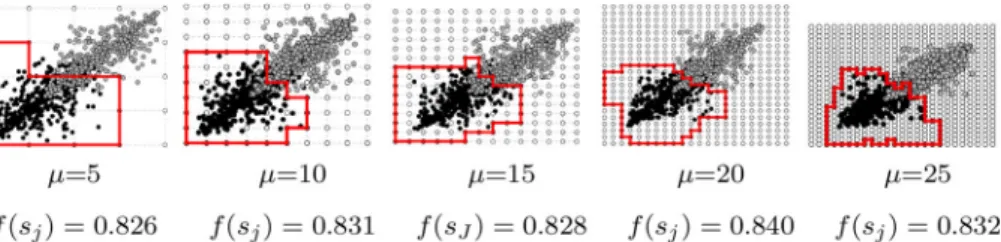
Fig. 4 Example of best known polygonsj∗for varying granularity factorμ. The parameterμcan be adjusted by the user
Gkmin=min(Ti jk)− (1)
Gkmax=max(Ti jk)+, (2)
whereTi jk represents an edge from nodeito node jat axisk.
The resolution of the graph environment can be manually adjusted through a granularity factorμprovided to the grid at initialisation.μ >2 is an integer that gives the granularity of the grid along both axes. For example, aμvalue of 5 would result in a 5×5 grid, a value of 10 would result in a 10×10 grid, etc. Since the graph is a square the resolution is the same for all axes. In other wordsμdetermines the granularity of the environment.
While a high granularity gives the ants more paths to choose from and the possibility to create more accurate solutions, it also increases the size of the search space and the time it takes for a single ant to complete its path. Figure4shows an example demonstrating that more fine-grained graphs can construct better classifiers than more coarse-grained graphs when given identical datasets.
After every completed ant walk, the pheromones in the graph environment are updated. The amount of pheromone laid in an area of the graph depends on the quality of the ant solution. The aim is to create a polygonsjthat surrounds all the items of classCjand does not surround any item of the opposite classes. The quality of a solutionsjis measured by a reward function f(sj)which is a function of the perimeter of the polygon and the number of elements that are correctly placed within it:
f(sj)=
ti∈Ch(ti,sj)
|C| , (3)
whereh(ti,sj)is a function that determines whether an elementti is on the inside of the solutions andC contains all items to be classified. PolyACO uses ray casting to determine if an element is on the inside or outside of a solution.h(ti,sj)is defined as follows:
h(ti,sj)= ⎧ ⎨ ⎩ 1 ifti∈Cj and is inside ofsj 1 ifti∈/Cj and is outside ofsj 0 otherwise, (4)
whereCjis the class represented by polygon (solution)sjso that a perfect solution surrounds all items of the classCjand no items of opposite classes.
In other terms, for an item that truly belongs to classCj according to its label and which is inside the polygonsj, it will geth(ti,sj)=1. For an item that does not belong to class
The function f(sj)includesh(ti,sj)for all items and thus reflects the homogeneity of items inside polygonsj.
To avoid overly complex polygons, we should favour polygons with smaller perimeters. This is achieved by modifying the reward function to be proportional to the inverse of the perimeter. Therefore, the smaller the perimeter, the higher the reward. The pheromone update can then be summarised utilising the following equations:
τi j← τi j+τi jbest τmax τmin (5) τbest i,j = f(sj) |sj| . (6) While this update form is similar to how pheromones are updated inMMAS, it includes factoring in the new reward function.
The current version of PolyACO has some weaknesses compared to other state-of-the-art classifiers. First, it is unable to classify data in more than two dimensions. Secondly, it does not handle classification problems comprising more than two classes. Thirdly, it is very slow and takes a long time to train.
2.3 Multi-levelling
Multi-levelling is a technique commonly applied to combinatorial optimisation problems as a way to efficiently search for solutions in a complex space. It involves recursive coarsening of complex problems to obtain a hierarchy of approximations to the original problem. An initial solution is found and then refined at each level as the problem space is coarsened (Walshaw2004; Lian et al.2015).
Adaptive mesh refinement (AMR) is a multi-grid technique used to dynamically modify the grid during computation by increasing the resolution of the grid in areas of interest (Berger and Colella1989). The strategy for selecting the grid areas in which to increase the resolution depends on the problem. AMR makes it possible to solve certain problems with a much higher precision level than traditional multi-grid methods as it requires less computing power than a uniform high-resolution grid. AMR has, for instance, been used to model the collapse and fragmentation of molecular clouds with an unprecedented accuracy (Klein1999).
2.4 Other classification schemes using ant colony optimisation
Several other classification algorithms using ACO and other metaheuristic algorithms are available in the literature.
(Salama and Abdelbar2016) use a cluster-based classification approach with ACO. They introduce a two-step approach. First, they assign a class to a cluster using ACO. Subse-quently, they continue using a local classifier which is independent of ACO. The approach introduces instance- and medoid-based ACO clustering and is basically an optimiser for existing classifiers.
The same authors introduce an approach for learning neural network structures using ACO (Salama and Abdelbar2015). Accordingly, they propose ANN-Miner to learn the structure of a feed-forward network, which in turn can be used to predict unknown classes of new patterns.
Varma et al. (2015) introduce NRSACO as a method for setting attribute reduction as an extension of rough sets theory. They claim that in contrast to standard rough sets, NRSACO is
able to avoid being stuck in local minima. This is similar to feature selection mechanisms using particle swarm optimisation, which aim at reducing the number of features for classification so that the classification becomes faster and easier (Xue et al.2014), and to how ACO is used for data reduction (Salama and Abdelbar2016).
An approach using ACO to optimise decision boundaries in decision trees is introduced in Sapin et al. (2015). Specifically, ACO is used to find nucleotide polymorphisms, which are then combined into a decision tree.
3 PolyACO+
PolyACO+ is an improvement of PolyACO which can handle an arbitrary number of dimen-sions and classes. It also drastically reduces the training time by computing the reward function in parallel on GPUs and by employing a dynamic multi-level scheme. This section describes the working of PolyACO+.2
3.1 Multiple-class classification
Figure5presents an overview of how PolyACO+ handles multiple classes. For example, when the number of classes is two, one polygon is sufficient to create a decision boundary. However, when the number of classes is larger than two, PolyACO+ creates one polygon per class. Since there are multiple polygons, an item to be classified belongs to three possible cases:
1. The item is located inside one polygon; in this case, the item is simply classified as the polygon to which it belongs.
2. The item is not located within any polygons; in this case, it is not possible to determine to which class it should belong. This problem is solved by simply accepting “no class” as a valid output from the classifier.
3. The item is encapsulated by several polygons; PolyACO+ handles this situation by ran-domly selecting to which class the item should belong. However, one consequence is that PolyACO+ classification becomes stochastic. An alternate option could therefore be to handle class conflicts by order of precedence. For example, given that the polygons from classC1andC2both surround a sample, then the sample is to be classified asC1
sinceC1has the lower index value. This action would produce an unjustified bias towards
polygons with low index values and might yield unexpected results.
3.2 Parallelisation with GPU
Based on recent advances from Tufteland et al. (2016), we now introduce GPU in the training phase. This is done by parallelising the most costly part of the algorithm, the reward function, to the graphics processing unit (GPU) using CUDA (Ryoo et al.2008).
Theh(ti,s)function combines all data points and edges in a training set. This set can be parallelised, which makes it well suited for a GPU kernel function. In practice, the GPU is invoked once per ant and returns a two-dimensional array of points in the training set and the number of edges produced by the ant. For more details, we refer the reader to Tufteland et al. (2016).
The two elements required for classification are the trained model and an implementation of the classification phase. The trained model in PolyACO+ is simply a description of the
Training Classification
Multiple ACO Ray tracing
Labeled data Polygons
Unknown items to be labeled Class 1: C1
Class 2: C2
Class 3: C3
Fig. 5 Overview of training and classification for PolyACO+ with multiple classes
Training Classification
Multiple ACO Ray tracing
Labeled data Polygons
Class 1: C1
Class 2: C2
xy-plane
xz-plane
yz-plane
Multiple ACO Ray tracing
Multiple ACO Ray tracing
Vote: C1
Vote: C1
Vote: C2
Classification: C1
Fig. 6 Overview of training and classification for PolyACO+ with several features
polygons constructed in the training phase. Although constructing these polygons is very computationally expensive, once they have been constructed they can be reused in the clas-sification phase. This phase is much less computationally expensive than the training phase and can therefore be implemented on other devices relatively easily.
3.3 Multiple features
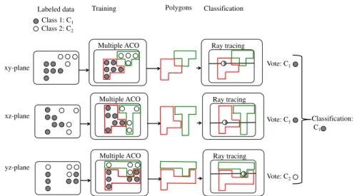
PolyACO+ supports multiple features by splitting a multi-feature classification problem into several two-dimensional sub-problems which are trained independently. The overall classification is a combination of the results from all sub-problems through a majority voting scheme. More precisely, the overall class prediction is derived by taking the most common class prediction from all the sub-problems, as illustrated in Fig.6.
3.3.1 Training
Instead of constructing solutions for only one plane as in the case of PolyACO, PolyACO+ constructs solutions in all the planes that the dataset consists of and handles each plane individually. The number of possible planes depends on the number of features in the dataset.
For example, a three-dimensional feature space with axesx,y, andzhas three planesxy,xz, andyz(see Fig.6). More generally, the number of planes for ann-dimensional feature space is simply equal to the number of dimension pairs and is given byn2.3
Further, the training phase constructs one polygon for each class in the dataset per plane. Thus, forvclasses andndimensions, the total number of polygons created by PolyACO+ is
n
2
×v. (7)
For example, for a dataset with 3 classes and 4 dimensions, the number of polygons in the training model is42×3=18.
3.3.2 Classification
PolyACO is a two-class classifier. PolyACO+ uses the concept of majority voting to extend PolyACO for handling multi-class problems. In order to classify a sample, each class is awarded a vote if it surrounds a sample in a given plane. For example, a class is awarded 2 votes if the polygons surround a sample in 2 different planes. The sample is classified as the class with the most votes when all votes are counted.
More formally, letti be an unlabelled item to be classified, andh(ti,s) is computed according to Eq.4:
h(ti,s)=
1 ifti is inside ofs
0 otherwise. (8)
The functionv(ti,k)counts the votes for a given sampletirelative to the classk.
v(ti,k)= p
i=0
h(ti,sk,j), (9)
wheresk,j is the polygon solution belonging to class k and plane j, and p is the total number of planes (see Eq.7). The votes for all classes k are gathered in a vectorvti =
(v(ti,0), v(ti,1), . . . v(ti,k))T. Finally, the predicted class for sampleti is defined as
p(ti)=arg max(vti), (10) where arg max(vti)is a function that returns the index of the largest element from vectorvti. In layman’s terms, PolyACO+ decides which class the item should belong by counting the number of polygons from each class surrounding the item.
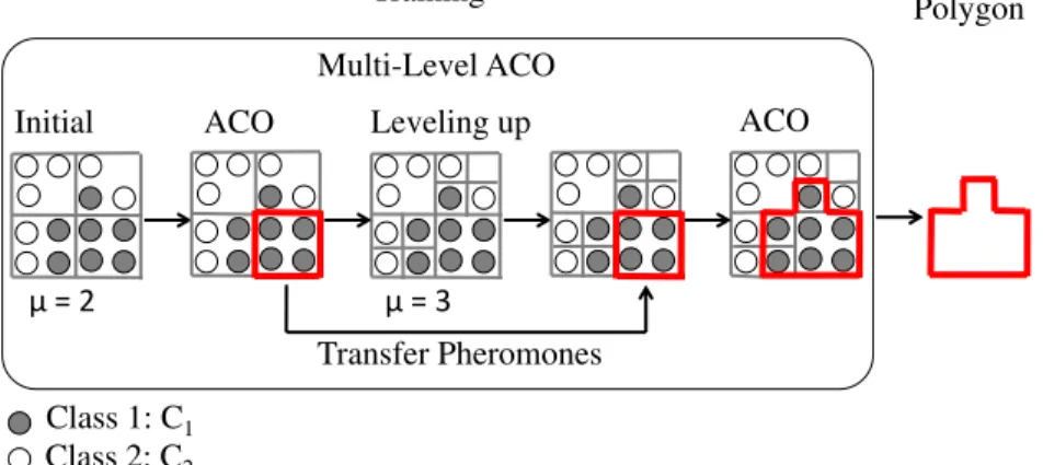
3.4 Multi-levelling
PolyACO+ is enhanced with multi-levelling capability and mesh refinement, which removes the need for manually tuning the granularity values of the grid. Following the principles of mesh refinement, the graph starts with a low granularity, for exampleμ= 3, and adaptively increases the granularity. The rise in leveling happens after the ants have converged onto a path according to the stop criterion, i.e. when no new solution is found for a fixed number of iterationsη. The pheromone trail is transferred over to the new graph, giving the ants an
3Inevitably, the number of planes grows exponentially with the number of features. However, feature selection
Training Multi-Level ACO Initial ACO Leveling up
Transfer Pheromones
ACO
Polygon
Class 1: C1
Class 2: C2
Fig. 7 Overview of multi-levelling in PolyACO+ with dynamic AMR
indication as to where the good paths are. The granularity is increased until a given maximum levelMis reached. At this point, when the ants converge, a solution is found. Figure7shows a concrete example of multi-level PolyACO+ fromμ=2 up toμ=3.
We present two alternative approaches to levelling in PolyACO+: a naïve multi-level approach based on traditional multi-grid techniques and a more sophisticated approach with adaptive mesh refinement (AMR) that intelligently selects in which part of the graph the granularity should increase.
3.4.1 Naïve multi-level
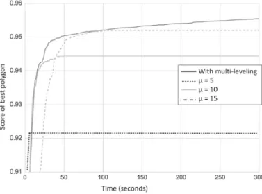
In the naïve multi-level approach, the grid is constructed initially with a low granularity and is “leveled up” by increasing the granularity on the entire grid when the ants converge. The convergence rate for a level is defined whenηants have not found an improved solution. Afterηants have walked without improvement, PolyACO+ levels up by splitting each edge into two new edges, and new edges and vertices are created in order to connect all vertices. During the experiments, the convergence rateηis set to 800.
Figure8shows the results of the experiment where we compare the results from a naïve multi-level run and a set of fixed granularity values. PolyACO+ with aμvalue (grid size) of 5 converges rapidly to one solution, and the found solution has the lowest score compared to the rest of the solutions. When we setμ=10, we see that the convergence speed decreases, but the quality of the solution increases. The case withμ = 15 yields an even slower convergence speed, but scores the highest of the three. Nonetheless, all solutions obtained by the fixed granularity approach are surpassed by the naïve multi-level approach in both score and convergence time. The figure also shows that the multi-levelling PolyACO+ produces better solutions after 300 s, long after the other approaches have converged. The full test results are presented in Table1, where we have also listed results obtained withμvalues of 30 and 60.
3.4.2 Multi-level with adaptive mesh refinement (AMR)
The naïve multi-level approach yields both increased accuracy and faster convergence speed. However, this comes at the cost of creating unnecessarily many edges and vertices in areas
Fig. 8 Naïve multi-level (average of 20 runs) Table 1 Quality (Eq.3) of naïve
multi-level after 15 and 300 seconds for different granularity levels
Granularity,μ Score, 15 s (%) Score, 300 s (%)
3 with multi-level 94.25 95.54 3 73.57 73.57 5 92.15 92.15 10 94.14 94.44 15 91.09 95.20 30 67.39 93.00 60 54.93 69.07
Bold indicates to highlight the highest performance in the corresponding column
where there are no training data. Those edges and vertices do not capture any points and therefore will only increase the search space and reduce the convergence speed. Instead of having a high granularity overall, a more desirable approach would be to have a higher level of granularity only in the areas that are covered by data points. This is achieved with multi-level AMR.
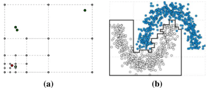
The local improvement works by recursively walking through the graph section by section. A section is defined as any four edges that form a square. Since a section is also a closed polygon, ray casting is applied to determine if a point is located inside or outside the section. If a section has data points of both the target class and of any other class, the section is divided into four new subsections. Figure9a, b shows a multi-grid with AMR on a simple constructed scenario, and a more complex semicircular dataset. The figures show how the grid is fine-grained in areas with data from both classes, and coarsely grained in the remaining areas.
AMR can be applied to PolyACO+ in two ways. The first approach is a static AMR where it is applied only once on training data and the outputted grid remains unchanged during the entire training phase. The second is a dynamic AMR where it is applied several times during training as illustrated in Fig.7. The dynamic approach starts with a coarser grid and then gradually increases the granularity over time. In this way, it can initially find good
(b) (a)
Fig. 9 AMR multi-level PolyACO+ applied to:aa simple example;bthe semicircular dataset
solutions very quickly and then refine these solutions in the next levels. Both the static and dynamic AMR approaches increase the granularity only in the most relevant parts of the grid. AMR approaches differ from the simpler naïve multi-level ones since the latter increase the granularity in the entire graph.
The dynamic AMR approach is used throughout this paper; all approaches are compared and discussed in Sect.4.6.
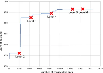
Convergence The stopping criterion in PolyACO is specified by the number of ants to run before stopping. The obtained solution is given by the ant path that has achieved the best score when the stopping criterion is reached. In PolyACO+ convergence is defined as when no new best solution is found for a given number of antsη. The intuition behind this stopping criterion is that the algorithm will not terminate as long as it is still finding new and better solutions. The convergence is per level, and when the convergence rate is reached at the final levelM, the algorithm terminates. Figure10illustrates the positive effects of the dynamic convergence in the multi-level approach. After each level-up (the crosses), the rate at which the algorithm finds new better solutions increases immediately. More productive levels, i.e. levels where better solutions are found frequently, are assigned more ants than levels where no better solutions are found. Regarding the example in the figure, we can observe that levels 3 and 4 are assigned more ants than levels 5 and 6, because they are more productive.
3.5 Early stopping
In order to improve efficiency, an optional early stopping criterion is applied by terminating earlier if the best polygon score does not improve for a given number of levels. For example, if the max levelMis set to 5 and early stopping convergence is set to 2 and the algorithm finds the best possible solution already at level 1, the algorithm will terminate at level 3 instead of level 5 for that particular polygon.
3.6 Multiple data points with shared coordinates
It is often the case that multiple data points share coordinates in a plane. For example, a two-by-two grid has only four possible coordinates. If the training set is larger than the number of possible coordinates, certain points must share coordinates. A problem occurs when the algorithm levels up: the granularity of a given section is increased if there are points of different classes within that section. In this manner, the grid is able to separate points of different classes without increasing the granularity on the entire grid. However, if points of different classes share coordinates, the multi-grid is never able to separate these points, even
Fig. 10 Multi-level AMS convergence in construction of a single polygon (η=2000,M=6, average of 20 runs)
with an infinitely high granularity. In order to handle this special case, PolyACO+ does not increase the granularity of a section if all points in the section share the same coordinate.
3.7 Additional enhancements
This section describes some additional enhancements to PolyACO+ compared to PolyACO. Equation6shows how pheromones are updated in PolyACO. This equation tends to bias the perimeter of the polygon compared to encapsulation of data points. This paper proposes an improved pheromone update equation using weights on the perimeter factor and data encapsulation, respectively: τbest i,j = f(sj)α· 1 |sj| β . (11)
For example, the significance of the length factorβcan be decreased by setting it to a low value.
All ants are initialised with a random position in PolyACO. Consequently, this might cause many ants to start in a position that is far away from any data point in the target class, making it hard to find good polygons around the target clusters. Therefore, two new methods for selecting the start position,WeightedandOn_Global_Best, are proposed. The
Weightedmethod selects a start position based on the amount of placed pheromones. The
On_Global_Bestmethod selects the current global best solution. Both approaches produced superior results compared to the random initialisation strategy. However, further investigation is needed in order to identify the best of the two approaches.
3.8 PolyACO+ parameters
Table2contains an overview of all the parameters of PolyACO+. The parametersρ,τmin,
Table 2 Overview of all algorithm parameters in PolyACO+
Name Description Default value
τmin Minimum pheromone value 0.001
τmax Maximum pheromone value 1.0
ρ Pheromone evaporation rate 0.02
η Convergence rate 1200
M Max granularity steps 6
α Weight for the reward function 1.0
β Weight for the polygon perimeters 0.01
Unless stated otherwise, the default parameter values from Table2are used in all experi-ments throughout this paper. These were obtained by testing various parameter values over a given number of ants on the generated semicircular dataset (see Sect.4.2.2), and then the best performing values were selected. This was done over several rounds for each parameter. For example, for the pheromone evaporation rateρwe first tested the values 0.001, 0.01, 0.1, and 1.0 and the results have been calculated with an average over 20 runs per parameter.ρ=0.01 performed the best. Therefore, we further tested the values 0.005, 0.02, 0.035, and 0.05. This time,ρ=0.02 performed the best and was therefore selected as the default value forρ.
4 Results
Experimental results are given in this section to demonstrate the efficiency of PolyACO+. We first start by presenting the synthetic and real data used in these experiments in Sect.
4.1. We continue in Sect.4.2by providing results from two featured datasets (including challenging problems such as circular datasets), while Sect.4.3is concerned with multiple-class multiple-classification with multiple attributes. Section4.4deals with fastening PolyACO+ using GPU, and Sect.4.5compares the results with other algorithms.
4.1 Data
This section presents results from various scenarios ranging from simple classification prob-lems using easily separable data to more complex settings involving both real-life and synthetic noisy data. For each generated scenario, 1000 data points per class are gener-ated. For the real scenarios, the whole corresponding dataset is used. The real datasets used in the experiments are Iris, Breast Cancer Wisconsin (bcw), and Digits4from the UCI dataset repository (Lichman2013). In all cases, half of the data are used for training and the other half for classification. All scenarios are run with 10,000 ants unless otherwise explicitly specified.
4.2 Two dimensions and two classes 4.2.1 Simple environment dataset
This section presents a simple experimental setting as a proof of concept of PolyACO+ in two dimensions. The aim of the experience is to empirically demonstrate that the approach
4Subset of “Pen-Based Recognition of Handwritten Digits Dataset (Lichman2013)” retrieved from
(a) (b) (c)
Fig. 11 Example of classification of the simple environment dataset.aPolyACO+ pheromones,bPolyACO+ polygon, andclinear SVM
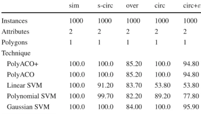
Table 3 Classification accuracy of PolyACO+ compared to state-of-the-art classification algorithms for the datasets simple environment (sim), overlapping data (over), circular (circ), circular with noise (circ+ε), and semicircular (s-circ)
sim s-circ over circ circ+ε
Instances 1000 1000 1000 1000 1000 Attributes 2 2 2 2 2 Polygons 1 1 1 1 1 Technique PolyACO+ 100.0 100.0 85.20 100.0 94.80 PolyACO 100.0 100.0 85.20 100.0 94.80 Linear SVM 100.0 91.20 83.70 53.80 53.80 Polynomial SVM 100.0 99.70 82.20 89.20 77.80 Gaussian SVM 100.0 100.0 84.00 100.0 95.90
works in a simple environment containing two easily separable sets of data. The data are composed of two sets of points:C1 andC2. Figure11a illustrates the pheromone trails at
the end of the training phase. The thicker the line, the more the pheromones deposited there, which means that the algorithm is more certain that the edge is part of the best solution. From the figure, we observe that the pheromones have built a rectangular polygon encircling all items inC1 without including any of the items inC2. Figure11b presents the best found
polygonsbased on the pheromone trail. Since this is a polygon that perfectly separates the classes, it yields f(sj)=1. The mapping from pheromones to polygon in this example is quite straightforward. Lastly, for comparison purposes, Fig.11c depicts the corresponding linear SVM. It is interesting to observe that PolyACO+ and SVM are able to find the same boundaries.
This simplistic example indicates that when it comes to easily separable data, the result of the PolyACO+ is similar to that of a linear SVM. Table 3shows an overview of the classification results. Both PolyACO+ and SVM reach an accuracy of 100.0—which is not surprising given the simplicity of the classification task.
4.2.2 Semicircular dataset
Figure12 illustrates the behaviour of the scheme in a more complex scenario involving semicircular data where there are no clear-cut boundaries.
Despite the added complexity, the PolyACO+ approach works almost identically to the simple scenario in Fig.11; Figure12a, b shows the pheromone trail and polygons, respec-tively, in the training data. We observe that there is an easy mapping from pheromones to polygon. Figure12c shows the boundary found by a linear SVM, which is not perfect
sim-(a) (b)
(c) (d)
Fig. 12 Example of classification of the semicircular dataset.aPolyACO+ pheromones,bPolyACO+ poly-gon,clinear SVM, anddpolynomial SVM
ply because the classification problem cannot be solved by a linear separator. Lastly, the polynomial SVM in Fig.12d produces better, but not perfect boundaries.
Table3shows that PolyACO+ achieves a classification accuracy of 100.0, while linear, polynomial, and Gaussian SVMs yield an accuracy of 91.2, 99.7, and 100.0, respectively.
4.2.3 Overlapping dataset
In the above scenarios, the data are perfectly separable. In the current scenario, the data in Fig.13are more challenging because they are overlapping and therefore no line or polygon can perfectly separate the datasets.
Figure13a shows the pheromones after the training phase. Concerning the left and lower parts of the polygon, the pheromone trail is strong and thus the lines are thick. In contrast, whenever the data overlap, the scheme is less confident and the pheromone trail is weaker. This indicates that when the confidence of the classifier is strong, PolyACO+ provides strong pheromone trails. Figure13b shows the corresponding polygon, and Fig.13c, d shows cor-responding boundaries of linear and polynomial SVM.
In Table3, we observe that PolyACO+ reaches an accuracy of 85.2, while linear SVM reaches 83.7, and polynomial SVM reaches 82.2. One conclusion to be drawn from this example is that PolyACO+ finds a slightly better boundary than SVM, presumably because the rigged lines better fit the data than the straight and polynomial lines.
4.2.4 Circular dataset
The classification tasks when the data points of a class form a circular shape are particularly difficult without mapping it to multiple dimensions. The data are generated from a Gaussian distribution from two circles having the same centre but with two different radii.
(a) (b)
(c) (d)
Fig. 13 Example of classification of the overlapping dataset.aPolyACO+ pheromones,bPolyACO+ polygon, clinear SVM, anddpolynomial SVM
Figure14a shows that the polygon is able to perfectly encircle classC1, which is only
matched by the SVM containing a Gaussian kernel in Fig.14c. The linear SVM in Fig.14b and the polynomial SVM (not presented as a figure) do not find any viable solution.
By adding 5% noise to the data, meaning that 5% of the data are intentionally wrongly labelled, Fig.14d shows that PolyACO+ is still able to obtain a nearly perfect solution.
Table3shows that PolyACO+ gets an accuracy of 1 compared to 53.8 for linear SVM and 89.2 for polynomial SVM. The PolyACO+ accuracy is only matched by Gaussian SVM. 5 In a noisy environment, the PolyACO+ algorithm has only marginally reduced level of accuracy, namely 94.8. Correspondingly, the polynomial SVM accuracy dropped from 89.2 to 77.8, while the accuracy of Gaussian SVM dropped to 95.9. Figure15shows the evolution of the score for the best polygons(f(sj)) and of the size of the polygon (|s|). Pheromones are represented by the edges’ width in the graph.
4.3 Multiple classes and features
This section presents classification results with PolyACO+ with multiple classes and features.
4.3.1 Number of polygons with multiple classes
We have carried out many experiments on multiple class problems. We present results for two real datasets, Iris and bcw (discussed further in Sect.4.5.1). Concerning this particular experiment, each dataset is run using three different values for the convergence rate and 50-fold cross-validation. A summary of results with many other datasets is available in Sect.
4.5.2.
5Note that the choice of kernel, including the Gaussian SVM kernel, is not trivial and typically relies upon
trial and error or expert knowledge of the field (Smola and Schölkopf2004). PolyACO+ has no such parameter to be tuned.
Fig. 14 Example of classification of circles.a PolyACO+ polygon,blinear SVM,cGaussian SVM, andd PolyACO+ polygon with 5% noise
(a) (b)
(c) (d)
Fig. 15 Evolution of polygon over time. Average of 1000 runs
Table 4 Classification accuracy levels using polygons for all and all-minus-one classes for different values of the stopping parameterη(100, 200, and 400)
Iris bcw
Convergence rateη 100 200 400 100 200 400
All-minus-one classes 90.40 93.20 93.84 97.28 97.03 96.79
All classes 92.44 94.12 95.28 96.92 96.92 97.12
The stopping criterion takes place whenever a number ofηants have walked without any improvement
The results in Table4demonstrate that while using all classes improves the classification accuracy levels on the Iris dataset, it does not produce the same effect on the bcw dataset. One possible cause for this discrepancy is that the data on the Iris dataset are continuous, while the bcw data are discrete. Figure16shows an example plane from the bcw dataset
Fig. 16 Polygons on sample planes from the bcw dataset for the classes grey (no-recurrent) and white (recurrent), and the Iris dataset for the classes grey (setona), white (versicolour), and black (virginica).abcw andbIris
compared with an example plane from the Iris dataset. The data in the bcw dataset are more uniformly distributed over the entire plane than in Iris. Therefore, in this manner, the classifier constructs polygons that cover the entire plane, instead of leaving large empty areas (as shown in Fig.16b). Since most of the plane is covered by polygons, little additional space is left for the class without a polygon, which reduces the risk of producing false positives.
The number of polygons constructed is a trade-off between precision and speed. Adding one more polygon per plane increases the total training time, but the gain in classification accuracy can be significant. The focus of this paper is more on classification accuracy than on speed. We adopted the all-class approach in this article, because the results in Table4
demonstrate that this method can provide improved classification accuracy, and the increase in training time is not very large.
4.3.2 Proof of concept for many dimensions
In this section, we demonstrate the training phase and classification phase in PolyACO+ using the Iris dataset as an example (see Sect.4.1). Iris has 3 classes and 4 features: sepal width, sepal length, petal width, and petal length. Iris has 4 dimensions, which produce 6 two-dimensional planes.
Figure17illustrates the dataset in each of the 6 planes. The surrounding polygons are produced during the training phase of PolyACO+. The colour of each polygon corresponds to the class to which it belongs.
The accuracy level in Table3is very close to all variants of SVM. With respect to the Iris Plant dataset the accuracy level for PolyACO+ is 95.2, compared to 97.2 for linear SVM and 99.7 for polynomial SVM. It is noteworthy that PolyACO+ reaches an accuracy level higher than AntMiner+ 94.5 and, not surprisingly, significantly higher than the two-dimensional PolyACO. This is a quite understandable result because using all four features produces higher accuracy than only using two.
Hence, assuming that SVM and AntMiner+ are able to classify the data well in an adept manner, it could be argued that the PolyACO+ algorithm does so as well.
4.4 GPU performance comparison
In order to measure the improvement of PolyACO+ by introducing GPU parallelisation, we ran an experiment comparing PolyACO+ with and without this component.
Fig. 17 Polygons for the Iris dataset in all planes with respect to classes grey (setona), white (versicolour), and black (virginica). The triangle is a potential new point to be classified.aSepal length vs sepal width,b sepal length vs petal length,csepal length vs petal width,dsepal length vs petal length,esepal width vs petal width, andfpetal length vs petal width
Table 5 PolyACO+ feature-by-feature comparison using tenfold cross-validation, measured in seconds used for training for Iris, bcw, and semicircular (s-circ) from 100 to 10,000 items
Iris (s) bcw (s) s-circ, 100 (s) s-circ, 1000 (s) s-circ, 10,000 (s)
PolyACO+ 113 162 6 7 8
PolyACO+ without multi-levelling 488 698 9 10 11
PolyACO+ without GPU 685 1956 15 77 676
The results in Table5show the runtime of PolyACO+ both with and without GPU paral-lelisation. The classification results themselves have been omitted from the table; as expected, they were very similar across all configurations. Applying parallelisation only changes the speed of the algorithm and not the classification accuracy. The gain in speed when using GPU is more significant when the size of the dataset increases.
Parallelisation reduces the runtime by a factor of up to 61.5x, which is a significant improvement compared with the original PolyACO (Tufteland et al.2016).
4.5 PolyACO+ compared to other classification algorithms
In order to test how well PolyACO+ performs on an overall basis, we compare it to state-of-the-art algorithms. Thus, in this experiment we compare PolyACO+ to logistic regression, SVM, neural networks, AntMiner+, and the original PolyACO. These algorithms were chosen because they either are very popular in the machine learning community or have similarities with PolyACO+. We used SVM and logistic regression implementations from the scikit-learn library and used Weka to run a neural network containing 2 hidden layers and a learning rate of 0.5. The AntMiner+ results are from the original AntMiner+ paper (Martens et al.2007).
The AntMiner+ results are run with tenfold cross-validation, while all other results are run with 100-fold cross-validation.6
4.5.1 Performance in higher-order dimensions
The training time of PolyACO+ drastically increases with increasing number of dimensions due to the increase in the number of two-dimensional planes. For example, in the case of 4 dimensions, the number of planes is only42=6, while for 1000 dimensions the number of planes is10002 =499,500. On Iris, PolyACO+ uses on average 17.67 seconds per plane to achieve good accuracy (95%±2%). Regarding a dataset with 1000 dimensions and equally many samples and classes as Iris, it would take approximately 100 days to complete a training phase.
In order for PolyACO+ to be practical to use in higher-order dimensions, some measures should be taken to either reduce the number of dimensions, e.g. through dimension reductions such as principal component analysis (PCA) and t-distributed stochastic neighbour embed-ding (t-SNE) (Van Der Maaten2014) or apply other data reduction methods (Varma et al.
2015; Salama and Abdelbar2016), or drastically increase the speed of the algorithm.
4.5.2 Results
Tables3,6, and 7show that the classification scores are very close to each other, with the exception of PolyACO. PolyACO+ scores the highest on bcw, while SVM obtains the best score on Iris and neural networks scores best on Digits. The original PolyACO has the lowest score on all the datasets. This is probably because PolyACO can only classify two-dimensional data, and therefore, it extracts only the first two features of each dataset and trains the model only based on them. It has a score of 10.18% on Digits, which is statistically equivalent to guessing as Digits has 10 classes. This is expected, since PolyACO only uses 2 out of the 64 features from Digits. Section4.5.3elaborates on PolyACO+ speed end convergence rate, including steps towards reaching an accuracy of 72.56% on the Digits data.
It should be noted that the best SVM set-up from the experiments in Table3 is, not surprisingly, Gaussian SVM. It is for this reason that we have included comparisons to Gaussian SVM in Table6.
Table6presents comparison results of PolyACO+ with other state-of-the-art algorithms on real datasets. For the purpose of comparison, we have included all obtainable data from Martens et al. (2007).7PolyACO+ produces a better accuracy level than all other algorithms for the three datasets Iris, bcw, wine, and better than all except Gaussian SVM for the bal dataset. However, more importantly, it is only outperformed by AntMiner+ with a large margin for three datasets (ttt, tae, and car), all of which have categorical features. For all other results, it reaches roughly the same, or significantly higher, accuracy level. The natural conclusion to be drawn is that AntMiner+ is superior to PolyACO+ for categorical data, and the opposite seems to be the case for datasets with continues numerical values.
Table 7shows accuracy categorised by data type (data containing categorical values, numerical values, and both).
6The AntMiner+ data are from the original AntMiner+ paper (Martens et al.2007) where experiments are
run with tenfold cross-validation. A higher cross-validation produces less bias towards overestimating the true expected error.
7Two datasets from Martens et al. (2007) could not be obtained because they are only available per request.
Table 6 Classification accuracy of PolyACO+ compared to state-of-the-art classification algorithms for the datasets Australian Credit Approval (aus), Tic-Tac-Toe Endgame (ttt), Contraceptive Method Choice (cmc), Teaching Assistant Evaluation (tae), Balance Scale (bal), Car Evaluation (car), wine, Iris, Breast Cancer Wisconsin (bcw), and Digits (dig)
aus ttt cmc tae bal car wine Iris bcw dig
Instances 690 958 1473 151 625 1728 178 151 699 1797
Attributes 15 9 9 5 4 6 13 4 9 64
Polygons 182 72 108 30 18 60 234 18 72 20160
Num/cat both cat both cat num cat num num num num
Technique PolyACO+ 85.52 65.80 45.05 49.70 87.43 69.91 99.32 95.20 98.05 78.28 AntMiner+ 84.05 99.75 45.93 56.73 79.81 92.01 94.59 56.73 96.40 – AntMiner 84.09 77.03 42.32 40.39 68.09 77.38 84.50 76.60 91.14 – AntMiner2 84.30 71.13 41.49 43.73 66.94 77.93 85.33 81.80 91.54 – AntMiner3 83.61 68.94 40.85 40.39 65.02 77.50 83.50 77.00 90.91 – RIPPER 84.52 97.99 48.94 35.30 79.38 94.01 90.68 93.00 95.35 – C4.5 84.82 83.79 46.60 47.20 77.11 96.61 89.83 93.80 94.69 – 1NN 80.33 98.50 42.16 50.20 81.83 92.69 95.43 91.00 96.40 – Logit 84.03 65.57 47.52 51.96 86.75 80.52 94.33 93.80 96.53 96.40 Gaussian SVM 85.22 91.06 48.55 48.42 91.58 97.71 94.83 94.40 92.81 94.01 Bold indicates to highlight the highest performance in the corresponding column
All data are from the UCI dataset repository (Lichman2013). Results other than PolyACO+ are from the original AntMiner+ paper (Martens et al.2007
Table 7 Average classification accuracy of PolyACO+ compared to state-of-the-art classification algorithms for datasets that only contain categorical values (cat), datasets that only contain numerical values (num), datasets that contain both categorical and numerical values (both), and average classification accuracy for all datasets (avg)
Technique cat num both avg
PolyACO+ 61.80 95.00 65.29 77.33 AntMiner+ 82.83 81.88 64.99 78.44 AntMiner 64.93 80.08 63.21 71.28 AntMiner2 64.26 81.40 62.90 71.58 AntMiner3 62.28 79.10 62.23 69.75 RIPPER 75.67 89.60 66.73 79.90 C4.5 75.86 88.86 65.71 79.83 1NN 80.46 91.17 61.25 80.95 Logit 66.01 92.85 65.78 77.89 Gaussian SVM 79.06 93.41 66.89 82.73
Bold indicates to highlight the highest performance in the corresponding column
Note that only PolyACO+, logit, and SVM have been tested on Digits. Therefore, Digits is not included in the comparison
Fig. 18 Confusion matrices for different classifiers. Each is run once on Iris. PolyACO+, polynomial SVM, and linear SVM reached accuracies of 98%, while the other two scored 96% in this example
The confusion matrices in Fig.18illustrate the precision obtained when classifying Iris using PolyACO+. When comparing this matrix to the other classifiers’ confusion matrix, we find that they all look approximately the same, which arguably supports the assertion that PolyACO+ works as well as comparable algorithms. Overall, the results from Tables3,6, and the confusion matrices strongly indicate that PolyACO+ is a competitive algorithm for solving classification problems when the features have numerical values. It is significantly more accurate than PolyACO and performs similarly or better compared to the other algorithms in the experiment. However, it is less competitive when it comes to categorical data.
4.5.3 Performance versus convergence rate
Figure19shows how the classification accuracy of PolyACO+ stabilises at a higher con-vergence rate on the datasets Iris, bcw, and Digits. The figure shows that while a higher convergence rate produces a higher classification accuracy, this accuracy is reached at dif-ferent levels for difdif-ferent datasets. This is in line with what might be expected as the datasets are of different complexity. Iris and bcw, which have 18 and 72 polygons, respectively, to optimise, converge forη≈300. In order to train PolyACO+ for the more complex dataset Digits, it is needed to include 20,160 polygons in the training phase, and the convergence rate clearly needs to be set higher. We would expect that by using a higher convergence rate, PolyACO+ would produce a higher level of accuracy, and it is therefore encouraging that the empirical evidence in Figure19supports this assertion.
4.6 Multi-level
This section compares the different multi-level approaches empirically. Each approach is run on the semicircular dataset from Fig.12. The semicircular dataset is a good choice to illustrate
Fig. 19 Classification accuracy when using an increasing convergence rate (η) for PolyACO+ on Iris and bcw (average of 50 runs) and Digits (average of 5 runs)
the effects of multi-levelling as there are clear boundaries between the class clusters in this case. The training phase is run for 100 seconds, and the best polygon is logged every second to monitor the progress. The four approaches in the experiment are as follows: a static grid with granularityμ =15, naïve multi-level, static grid with AMR, and dynamic grid with AMR.
A value ofμ=15 was empirically tested to give PolyACO+ the highest accuracy without multi-level (see Fig.8) and is included in Fig.20. The results in Fig.20show that the naïve multi-level approach converges earlier than the static grid approach with a fixed granularity, and at the same time lower than the two versions using AMR. Similarly, static AMR converges earlier than dynamic AMR, but with a lower score. This is because the static grid has a max level of 4, meaning that it has a small and limited search space. In this way, it not only converges very fast, but is not able to separate the data as well as the dynamic approach.
4.6.1 Discussion
The naïve approach consists of applying traditional multi-grid techniques by increasing the granularity on the entire grid when ants converge and pass on the pheromone values from the coarse grids to the finer grids. Another approach is to apply AMR by only increasing the granularity in areas of relevance. This approach can be applied either once at initialisation of the grid or dynamically during training. All multi-level approaches obtain very good results compared to no multi-levelling. Dynamic multi-levelling with AMR shows superior results compared to the other approaches and is therefore the preferred technique for PolyACO+. Moreover, the performance is further increased by applying a dynamic convergence which assigns more computing time to productive grid levels than to unproductive grid levels.
Fig. 20 Multi-level comparison (averaged over 50 runs) Table 8 Performance overview for Digits (average of 5 runs)
Convergence rate Average accuracy Average time per run (h) Time per polygon (s)
η=300 72.55 69.6 12
η=500 72.89 112.4 20
η=800 78.28 139.8 24
4.7 Performance on the Digits dataset
Table6shows that PolyACO+ scores considerably lower on the Digits dataset than the other classification algorithms. This could be explained by the fact that the Digits dataset is more complex than the others, as it contains 64 features and 10 classes, resulting in a total of 20,160 polygons in the classification model (see Eq.7).
Figure19and Table8confirm that increasing the convergence rate also increases the accuracy level. However, this takes place at the expense of slower convergence since a higher convergence rate means increasing the number of ants.
4.8 Discrete, continuous, and categorical values
Table7shows the results for each classifier grouped by data type. When the data are purely numerical, PolyACO+ beats all algorithms in our comparison. In contrast, when the data are only categorical, AntMiner+ is the best performing algorithm. When the data contain both numerical and categorical values, SVM becomes the best performing algorithm, but it is noteworthy that PolyACO+ is better than AntMiner+ in this case. One conclusion to be drawn from this is that PolyACO+ works best and is the best among the compared algorithms, when the dataset contains numerical values. Without numerical values, PolyACO+ should not be the chosen classifier.
(a) (b) (c)
Fig. 21 Example of a multi-grid inacontinuous domain, Iris, andbdiscrete domain, bcw, andccategorical data, car
Figure19shows that PolyACO+ stabilises at a lower convergence rate on the bcw dataset than on Iris and Digits. PolyACO+ achieves an average of 93.5% accuracy on bcw with
η=10, while it only achieves a 76.6% accuracy on Iris with the same settings.8The main difference between Iris and bcw is the number of features (4 and 9, respectively) and the type of values in the data: bcw only has discrete values between 1 and 10, while Iris has continuous values with no particular constraints. The multi-grid in PolyACO+ is a discretisation of the entire dataset and is therefore quite congruent with discrete values. Figure21illustrates the difference between multi-grids based on continuous data and on discrete data. The grid can more easily separate the discrete data as it does not require a high resolution before each unique data position has a separate section in the grid. The continuous data require a very high resolution to separate the points, because the values can be much closer to each other than in a discrete domain.
In order to explain the limitations of categorical data for PolyACO+, we use the example of the categorical dataset car. Applying PolyACO+ to the car dataset produces an accuracy level of 69.9, compared to 92.0 for AntMiner+.9The car dataset consists of 6 features, all of which are categorical. PolyACO+ by design expects numerical values for the features in a grid and not categorical features. We counter this problem by mapping every possi-ble value in a category to a binary 0–1 category. For example, feature maintenance in the car dataset has 4 possible values: vhigh, high, med, and low. This is instead mapped to 4 features: maintenance_vhigh, maintenance_high, maintenance_med, and maintenance_low. Figure21c shows a plot of maintenance_vhigh (x-axis) versus maintenance_high (y-axis). It is observable from this example that each items falls into either maintenance_vhigh, maintenance_high, or neither, and there is an exact overlap between these categories. Since PolyACO+ works in two-dimensional plots alone, there is not a very good separator from these features alone. Further, since the car dataset only includes categorical data, this is true for any subset of two features, and PolyACO+ does not perform that well in this situation.
5 Conclusion and further work
In this paper we have introduced PolyACO+, a classification algorithm which is a significant extension of the PolyACO algorithm that uses ant colony optimisation and ray casting for classification. PolyACO+ introduces several modifications and improvements to PolyACO,
8Note that after convergence, the accuracy is much higher as presented in Table6.
9Note that for the continuous datasets, e.g. Iris, we observe the opposite case and PolyACO+ outperforms
such as the capability to handle multidimensional data, support for multiple classes, and an efficient parallel architecture for GPUs that improves accuracy and speed.
PolyACO+ employs a novel approach to handling multidimensional data where a sep-arate classifier is trained individually for each pair of features. Subsequently, PolyACO+ uses ray casting and majority voting to construct an aggregated classification decision. The approach is successfully applied to multiple multidimensional datasets such as the bcw and Iris datasets. The algorithm performs similarly or better than state-of-the-art algorithms with an average classification accuracy of 95.20% on Iris and 97.11% on bcw. Moreover, Poly-ACO+ outperforms all other classification algorithms, including neural networks and SVM. Since bcw consists of discrete data, this suggests that PolyACO+ works particularly well for this type of data.
To reduce the complexity per dimension, PolyACO+ also applies adaptive mesh refine-ment. This multi-level technique works by increasing the granularity in parts of the graph with denser data while keeping lower granularity in parts where the data are sparse. In this manner, the ants do not have to spend time in areas which do not give added value.
Overall, PolyACO+ performs well on all our experiments with continuous and discrete numerical values and meets our objectives in terms of improving PolyACO. We therefore conclude that PolyACO+ is a viable technique for solving classification problems. Concerning categorical data, PolyACO+ falls short compared to other classifiers specialised for this type of data, for example AntMiner+.
One of the biggest drawbacks of PolyACO is the fact that it is slow. In order to circumvent this disadvantage, PolyACO+ employs a parallel architecture for the reward function that can run on GPUs. The runtime of the reward function is reduced using parallelisation, which reduces the overall running time of the training phase to between 16 and 1.6% of its original runtime.
PolyACO+ is still relatively slow compared to other classical algorithms. The reason for this is that the number of polygons increases quadratically with respect to the number of features.
Two strategies might improve the performance further: first, extending parallelisation to other parts of the algorithm and second, resorting to smart dimension reduction techniques. Potential approaches include adding a kernel functionality similar to how SVM uses kernels (i.e. smart exploration of relevant and non-relevant dimensions), and letting the ants walk in multidimensional planes. The viability of these approaches needs to be explored.
The paths in PolyACO+ are composed strictly of horizontal and vertical edges, and the distance along a path is computed using the Manhattan distance. Two paths that are of the same length calculated with the Manhattan distance may be of different lengths in Euclidean geometry. The combination of PolyACO+ and a Euclidean geometry would permit diagonal lines and allow a greater variety of polygons. Whether or not Euclidean-based PolyACO+ would improve the algorithm accuracy needs to be explored.
There are multiple ways of countering the Manhattan distance problem. One solution is to use the area of the polygon instead of the perimeter in the reward function. However, this approach could pose a challenge, as calculating the area may be computationally expensive, while calculating the polygon perimeter is trivial. Another approach would be to introduce diagonal edges. This solves the problem of Manhattan distance, but comes at the cost of making the computations on the graph more expensive. Moreover it could be challenging to implement the latter solution for asymmetric grids including the adaptive mesh refinement grid used in PolyACO+.
Other mechanisms we intend to explore are multiple polygons per class per pair of dimen-sions and weighing of each polygon as both mechanisms would allow the detection of more