A warranty forecasting model based on piecewise statistical distributions and stochastic simulation

(1)

A warranty forecasting model based on piecewise statistical distributions

and stochastic simulation

Andre Kleyner

a,

*, Peter Sandborn

b a_{Delphi Corporation, P.O. Box 9005, M.S. R103, Kokomo, IN 46904, USA}

b_{CALCE Electronic Products and Systems Center, Department of Mechanical Engineering, University of Maryland, College Park, MD 20742, USA}

Received 11 May 2004; accepted 27 July 2004 Available online 25 September 2004

Abstract

This paper presents a warranty forecasting method based on stochastic simulation of expected product warranty returns. This methodology is presented in the context of a high-volume product industry and has a specific application to automotive electronics. The warranty prediction model is based on a piecewise application of Weibull and exponential distributions, having three parameters, which are the characteristic life and shape parameter of the Weibull distribution and the time coordinate of the junction point of the two distributions. This time coordinate is the point at which the reliability ‘bathtub’ curve exhibits a transition between early life and constant hazard rate behavior. The values of the parameters are obtained from the optimum fitting of data on past warranty claims for similar products. Based on the analysis of past warranty returns it is established that even though the warranty distribution parameters vary visibly between product lines they stay approximately consistent within the same product family, which increases the overall accuracy of the simulation-based warranty forecasting technique. The method is demonstrated using a case study of automotive electronics warranty returns. The approach developed and demonstrated in this paper represents a balance between correctly modeling the failure rate trend changes and practicality for use by reliability analysis organizations.

Keywords:Stochastic simulation; Warranty analysis; Piecewise distribution; Monte Carlo; Automotive warranty forecasting; Weibull analysis

1. Introduction

Market conditions have traditionally been the main factor that determines the terms of automotive warranties. While expected reliability and quality of the product is considered an important supporting factor, in reality, the actual warranty terms are most often determined by marketing pressures. Currently the terms of the standard automotive warranty, often referred to as the manufacturer’s basic warranty are 36 months or 36,000 miles (whichever comes first) on the majority of vehicle parts (see, for example, [1]) with additional extended warranties on selected subsystems. Longer warranty periods are often used as an enhanced marketing tool; warranty history

and warranty expectations greatly affect the market value of new and used cars sold, and lease residual values. Because of these and other financial and marketing considerations, a multitude of business decisions are being made based on the forecasted number of warranty returns for the overall warranty period and subsets thereof. All the aforementioned makes the process of improving warranty claims forecasting even more important, further increasing the need for models that provide an acceptable accuracy for business decision making. In addition, a parallel need for warranty forecasting in industry also arises when the first few months of warranty claims are being analyzed for the purpose of forward extrapolation and development of appropriate corrective actions.

In many industries quality and reliability engineers who are involved in the warranty forecasting process use empirical models based on past warranty claims of products with similar design and complexity adjusted by certain, 0951-8320/$ - see front matterq2004 Elsevier Ltd. All rights reserved.

doi:10.1016/j.ress.2004.07.016

www.elsevier.com/locate/ress

* Corresponding author. Tel.:C1 765 451 8070; fax:C1 765 451 9874. E-mail addresses: [email protected] (A. Kleyner), [email protected] (P. Sandborn).

(2)

experience-based correction factors accounting for the

design and technology changes in the product.

A reasonably accurate, scientific, and user-friendly model could help to accomplish warranty prediction tasks with better precision and improve the overall quality of business decisions requiring estimates of future warranty claims.

2. Warranty forecasting model

In this paper, we will cover the two most common types of warranty forecasting activities. The first type includes future product estimates, which are usually conducted in a product planning stage in order to anticipate the costs associated with future warranty returns. This type of analysis is based on the product complexity, technology, and other design aspects known in advance about the product. The second type is the ongoing forecasting for current products, where the warranty returns are known for the first few months of service and the objective is to anticipate the final numbers of warranty returns at the end of the warranty cycle and beyond.

Warranty data usually contains information on all incidents reported during the warranty period. It is conventionally accepted that product failure behavior can be modeled by a ‘bathtub curve’ that is widely used in reliability literature [2]. There exist a variety of math-ematical models that adequately represent the reliability bathtub curve[3–8]. For our purposes we are interested in a model’s ability to fit the data presented in the automotive warranty reporting formats described in Section 3. Many bathtub-curve models are mathematically expressed in terms of hazard rates (or failure rates), while reliability engineers are usually more accustomed to working with reliabilities and percentages of failures. Also since reliability forecasting is usually the ultimate goal of this kind of analysis, a model expressed in terms or reliability would typically be easier to apply directly in engineering calculations.

Based on the fact that a typical automotive part is designed for a mission life of 10–15 years, it is very unlikely that it would be subjected to wear-out failures during either warranty or extended warranty periods of 3–7 years.

Fig. 1 provides an illustration of an automotive electronics product family failure rates recorded in terms of incidents per thousand vehicles (IPTV) see Eq. (1) for seven different model years1 of the same product family (model years A–G inFig. 1). The data shows no wear-out mode for at least the first 4 years of service

IPTVðtÞZClaims

ðtÞ

NðtÞ 1000 (1)

where

Claims(t)Znumber of claims reported in the periodt.

N(t)Znumber of vehicles in the field in the periodt.

For any time interval T the relationship between IPTV and conventional failure rate would be:

lðTÞZIPTVðTÞ

1000T (2)

wherel(T)Zfailure rate for the time intervalT.

Fig. 1 suggests that in the majority of the cases the warranty failure model is sufficiently represented by the infant mortality and useful life phases of bathtub curve.

A detailed study of the existing warranty of various product lines of automotive parts performed at Delphi Corporation showed a clear trend of diminishing failure rate for the first 8–18 months (seeFig. 2) followed by a flattening of the failure rate curve for the remainder of the time period where warranty and extended warranty data were available. To combine the first two sections of the bathtub curve and to provide a best fit for the warranty data inFig. 1 or Fig. 2we suggest using a conditional reliability equation RðtÞ_ZRðtsÞRðts/tÞ ðtOtsÞ (3)

where

R(t)Zreliability at the time intervalt.

tSZpredetermined time coordinate.

R(tS)Zreliability at the timetS.

R(tS/t)Zprobability of reaching the time pointt, under

the condition that timetShas already been reached.

As mentioned earlier, most of reliability and quality engineers are more accustomed to working with reliabilities expressed in terms of commonly used distributions: Weibull, Exponential, Normal, and Lognormal. Analysis of the existing data (Fig. 2) shows thattS, can be determined

as the time coordinate where hazard rate stabilizes, and the failure data with decreasing failure rate in the range [0; tS]

could be fitted by Weibull distribution. Similarly the failure data in the range [tS; t] could be fit with Exponential

distribution, since the failure rate would remain relatively constant in this range. This approach is similar to the method discussed in[9], where the combination of Weibull and Exponential distributions were used to calculate the expected MTBF of a hard disk drive. Under the piecewise scheme described above, (3) becomes

RðtÞ_ZeKðts=hÞb_eKlðtKtsÞ; _t_R_t

s (4)

where

bZWeibull slope often referred as shape parameter. 1

Model year is a manufacturer’s annual production period. In the automotive industry new model year production may start as early as July of the previous calendar year.

(3)

hZWeibull scale parameter, often referred as

character-istic life.

lZconstant failure rate aftertS.

The time tS can be referred as a change point, the

coordinate where the pattern of data changes requiring a different data-fitting model [10]. The continuity at

the junction point tS can by achieved by equating the

hazard rates at the point tS. The hazard rate for Weibull

distributionhWeibullattSis:

hWeibullðtsÞZ b ts t_s h b (5) Fig. 1. Extended warranty charts compiled from Delphi Corporation warranty data for the several model years of the same electronic product mounted in the engine compartment of an automobile.

Fig. 2. Failure rates expressed in incidents per thousand vehicles (IPTV) for selected passenger compartment mounted electronic products recorded by Delphi Corporation. The actual IPTV values have been modified to protect the proprietary nature of the data.

(4)

Thus equatinghWeibullwith the constant failure ratelpast

the pointtSwould produce:

lZ b ts ts h b (6) The overall reliability expressed in (4) has four parameters: b, h, tS, and l, using (6) to eliminate l, (4) can be

transformed into: RðtÞZexp K 1C bðtKtsÞ ts _t s h b " # ; tRts (7)

Eq. (7) is in a suitable format for a stochastic simulation such as Monte Carlo analysis, which has been successfully applied in a variety of parametric studies of reliability[11]. Each of the parameters, b,h,tS, is a random variable and

could be represented by a statistical distribution. The best way of obtaining those distributions is by observing the past history of the product. The authors studied warranty returns for several automotive electronics product families and identified some common trends in the data. While the variation of statistical parameters between those groups was significant, parameter variation within the same product group was far less apparent. An important factor governing variation within a product family was found to be the number of years in production with a tendency for the first year to have the highest number of warranty claims.

Besides forecasting the expected warranty returns for future products, this model can also be used for ongoing forecasting of current products, where the final warranty prediction is based on the number of claims reported after the product’s first few months in the field and is subject to continuous updates. This type of forecasting is often used to compile monthly reports to the management as well as to detect potentially serious field reliability problems.

3. Determining the distribution parameters

In this paper, we are going to consider two data formats commonly used for automotive warranty data reporting. In the first format, the data is presented in ‘30-day buckets’ where the failure data is divided into 30-day service time intervals counted from the date of vehicle sale, where all the failures occurring within each 30-day time interval are reported in failed quantities or IPTV. The IPTV format (see example inTable 1) is an easier, faster, and more common

form of data reporting and is usually sufficient for the first-level approach to data analysis. The raw warranty data typically contains additional information including vehicle identification number (VIN), vehicle mileage, geographical information, cumulative costs, cumulative IPTV, and many other parameters.

If the failed units can be traced to a specific production lot, this data can be converted into a more comprehensive format sometimes referred by quality professionals as ‘layer cake’, which usually combines all sold and failed units on a monthly basis, as presented in the Table 2. This format provides information, which allows the user to trace each failure to a particular production group and can be used to conduct more sophisticated statistical analyses.

The actual data in Tables 1 and 2 was made up for example purposes and is not linked to any real product or to each other. The format inTable 2is easier to understand and data in this form can be easily processed with commercially available software like WeibullCC from ReliaSoft Cor-poration[12]and be converted into interval-based life data. Both formats discussed above are acceptable for obtaining the distribution parametersb,h,tS, however, the

30-day bucket data can be analyzed only on a percentage-failed basis and is thus unusable for the calculation of confidence bounds. In contrast, the layer cake data provides more options for determining a best-fit distribution includ-ing the estimation of confidence bounds. However, it is important to mention that the 30-day bucket format can be considered as a cost/time saving version of layer cake since it involves fewer data processing steps.

The procedure for determining distribution parameters starts with obtaining the change point estimation tS. Since

any real data would demonstrate some form of variation between consecutive 30-day intervals, we suggest using the Bayesian smoothed hazard function described in [13]. It would modify the stepwise pattern of the interval-based hazard function and would provide a continuous transition between adjacent 30-day intervals using Bayesian esti-mation of hazard rates. For simplicity purposes the average hazard ratehavg(t) given by Eq. (8) can also be used for this

type of analysis: havgðtÞZ

Number of accumulated failuresðtÞ

Total accumulated time in serviceðtÞ (8)

Graphic analysis of the average hazard rate shows the general trend of saturation starting attS. One of the criteria

Table 1

Example ‘30-day Bucket’ data Days in

service

Vehicles in the field during the time period

Reported number of failures

IPTV (incidents per thousand vehicles)

1–30 10,000 8 0.80

31–60 9000 2 0.22

61–90 7000 9 1.29

Table 2

Example ‘Layer cake’ data

Month New vehicles sold Number of failures by month

Month 1 Month 2 Month 3 Month 4

1 15,980 5 3 12 1

2 23,340 5 7 12

3 26,541 6 1

(5)

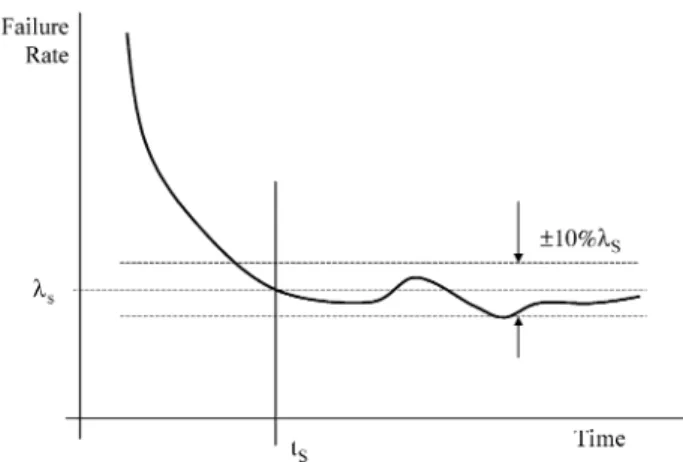
used for determining the exact change pointtScould be the

flattening of the curve to fit withinG10% of the boundaries of the saturated hazard rate value as shown inFig. 3(other criteria may be practical depending on the specific nature of the data and the shape of the curve).

If the characteristics of the data are different from that presented inFig. 3and do not have a pattern of diminishing failure rate followed by stabilization, then the parametertS

can be estimated from visual observation of the plotted data whenever possible. The majority of the datasets initially studied by the authors (42 out of 45) did exhibit the stabilization trend. The remaining three cases did not display the similar pattern being special cases with assignable causes of failure. For that reason they were considered outliers and were not included in the pool of datasets used for evaluation of distribution parameters oftS.

Procedurally for each set of data the failure numbers should be split into pre-tSand post-tSintervals. Then each of

the two data sets should be Weibull-fit as a separate group for determining Weibull parametersbandh. Analysis of the product groups mentioned previously, demonstrated stable trends, showing that the pre-tS Weibull slope b (we will

refer to it asb1) typically stays in the range of 0.65–0.85.

The statistical analysis of more than 40 different data sets with the @Risk software package[14]demonstrated that a two-parameter Weibull distribution was indeed the best-fit distribution for the pre-tSdata in almost half of the cases.

For the remainder of the datasets Weibull was in the top five out of 28 different distribution options thus supporting the choice of Weibull distribution for this procedure. The similar analysis of post-tSdata showed that Weibull slopes

b2in all analyzed cases were withinG10% ofb2Z1.0, thus

confirming the constant failure rate assumption for the post-infant-mortality stage.

4. Forecasting procedure

Two separate procedures are suggested for the two data formats mentioned in Section 3. Both can be

performed using commercially available reliability anal-ysis software.2

The data presented in layer cake format allows more sophisticated data processing, since the user is able to obtain exact failure time intervals and the number of suspended items. This more detailed information allows the implemen-tation of Maximum Likelihood Estimator (MLE) Weibull analysis or other distribution best-fit approaches and provides the confidence intervals on the results of the best-fit approximation. It is also important to address the effect of the production year. For example, it has been observed that quality usually improves with the number of years in production due to continuous improvement of manufacturing procedures. Thus the obtained b and h coefficients can be categorized not only by product features, like model numbers, functionalities, car platforms, etc. but also by the number of years in production for the same product group.

It is also important to mention the multi-dimensional aspect of warranty specifications. Since automotive warran-ties are usually expressed in both time and mileage terms, i.e. 36 months or 36,000 miles whichever comes first[1], it is a two-dimensional warranty[15], which can be accounted for by using the methodologies presented, for example, in Refs. [16,17]. For automotive electronic parts it is more appropriate to use time as the primary usage variable since there are no moving parts involved in the process of wear-out, though the mileage variable is also important in estimating the expected warranties. Any of the method-ologies described in the referenced literature can be applied to the proposed model in order to add an additional dimension of warranty. For example, if warranty is expressed in terms of {T0, M0} with T0 being specified

maximum time period andM0specified maximum mileage,

and if we can obtain the probability distribution function of reaching mileageM0at timet,f(tjM0), then

FðTÞWarrantyZ

ðT

0

½1KRðtÞfðtjM0Þdt (9)

where F(T)_WarrantyZfraction of accumulated failures cov-ered by warranty for the time periodT.

Or after substituting (7) into (9):

FðTÞWarrantyZ ðts 0 ½1Ke Kðt=hÞb fðtjM0Þdt C ðT ts 1Kexp K 1C bðtKtsÞ ts _t s h b " # " # !fðtjM0Þdt; TRts ð10Þ

Fig. 3. Change point estimation fortS,lSis the failure rate attS.

2

When using ReliaSoft WeibullCCwith the ‘30-day bucket’ format it

is best to use a ‘free form data’ format, which is made up ofXtime to failure data andYposition data in % in which ranks are not assigned to the times. The solution method is least squares (rank regression inXorY). The time interval (30-day 60-days, etc.) would represent theX-axis and 0.1!IPTV

(6)

Procedurally, each trial in the Monte Carlo simulation would include solving the integral (10) for every generated set of random variablesb,handtS.

In addition, (7) can be used for ongoing warranty forecasting for current products. Direct application of Eq. (7) in conjunction with (10) allows using pre-tSdata (data

from several months of warranty return) to predict the post-tSdata expanding to the normal warranty period, extended

warranty period, and beyond.

5. Automotive electronics application example

For simplicity we will consider only the data presented in 30-day bucket format. Let us assume that we must forecast the 5-year/50,000 miles extended warranty of the new passenger compartment mounted product and let us also consider the effect of production start (usually the first year production) on the rate of returns for this part. The warranty data is available for four different models with similar features and complexities. Due to limited space we will present the initial data for only one model called Product 1, 1st year production lot (Table 3), and show the rest of the data in a statistical distribution format. As before, the presented warranty numbers will be altered due to proprietary nature of the data.

Since the data comes in 30-day bucket format it is best to apply the free form data format (percentages failed) to pre-tS

(b1) and post-tS(b2) separately.

Typically the type of information presented inTable 4 would contain a much larger amount of data with more automotive product categories due to the large number of parts and applications. For instance, the same models can be subdivided by vehicle platforms, where the same type of products would be considered as a different group if they were installed on light trucks as opposed to mid-size cars. The larger the number of similar product lines, the better the confidence intervals for the results obtained with Monte Carlo simulation.

There are several possible ways of processing the data presented in the Table 4. All the data can be analyzed together by finding the best distributions for each of the three parameters b1, h, tS, and based on the obtained

distributions, model those values for Monte Carlo simu-lation with (7) or (10). However, if we are, for example, interested in the warranty of the product manufactured within the first year after the start of production, only the data pertinent to the first year of production will be analyzed (see the four bold rows inTable 4). Based on these four data groups the following distributions were obtained: tS Lognormal distribution:mZ5.71,sZ0.186

b1 2-parameter Weibull distribution: bZ6.62, hZ0.815

(please note that those are the distribution parameters of b1, and not that of the original failure data)

h1 Normal distribution:mZ247,830,sZ30,069.

In order to account for the effect of two-dimensional characteristics of warranty we need to estimate the probability distribution function f(tj50,000 miles) of mile-age reaching 50,000 miles at time t. First, using the dealership data containing the analysis of dates and mileages associate with each warranty claim we can construct a probability distribution function of daily mileage fDaily(m). Our data was based on the sample of 1000

warranty claims containing both time and mileage infor-mation that was best-fit with two-parameter Weibull distribution with shape parameter bZ1.55 and scale

parameterhZ41.1 miles (66.1 km). Using those parameters

we obtained a conditional probability distribution f(tj50,000 miles), which is based on daily distribution mileage above and is best represented by Lognormal distribution with parameters:m_Z7.53 ands_Z0.904.

A 10,000 sample Monte Carlo simulation of expected warranty returns at the 5-year mark (1825 days) produced the following results according to Eq. (10).

Mean value for cumulative return of claims covered by warranty wasF(5 yr)Z2.2% (50% confidence). With upper

80% confidence this value reachingF80%(5 yr)Z3.1%.

Table 3

Product 1 (1st year production lot)

Days in service IPTV Total % failed

0–30 3.03 0.30 31–60 1.50 0.45 61–90 1.41 0.59 91–120 1.39 0.73 121–150 1.32 0.87 151–180 1.31 1.00 181–210 1.37 1.13 211–240 0.49 1.18 241–270 0.36 1.22 271–300 1.70 1.39 301–330 0.45 1.43 331–350 1.70 1.60 361–390 1.76 1.78 391–420 1.74 1.95 421–450 0.65 2.02 451–480 2.90 2.31 481–510 0.92 2.40 511–540 2.80 2.68 541–570 0.30 2.71 571–600 1.20 2.83 601–630 0.20 2.85 631–660 0.15 2.87 661–690 0.55 2.92 691–720 2.40 3.16 721–750 0.60 3.22 751–780 2.00 3.42 781–810 2.50 3.67 811–840 0.90 3.76 841–870 5.00 4.26 871–900 3.27 4.59 901–930 1.12 4.70 931–960 0.21 4.72

(7)

This example demonstrates the use of (10) with real data to perform a reliability/warranty prediction. A common simplistic method to treat the data associated with this example would have been a Weibull analysis of early failures for existing parts with similar design features. In our case, a simple Weibull analysis of early failure data that accounted for the 2-D aspect of the warranty would produce F(5 yr)Z0.74%, which is significantly lower than the result

obtained from Monte Carlo simulation using (10). Weibull analysis of the early failures often presents an over-simplification of the science that does not capture the trend change in the failure rate. Alternatively, detailed statistical approaches[3–8]adequately represent the bathtub curve, but are not formulated for forecasting and are generally not practical for use with real data and its associated uncertainties.

6. Conclusions

The model presented here offers a straightforward solution to a complex two-dimensional warranty prediction problem. The solution is easy to implement within Monte Carlo or other types of stochastic simulations because it is represented by a single closed-form equation. The pro-cedure allows the user to practically accomplish two major reliability prediction tasks: (1) the forecasting of future product warranty at a product planning stage, and (2) the ongoing forecasting for current products, where the warranty returns are known for the first several months of production. This method can be used to predict the number of failed parts, which would not be reflected by warranty claims due to mileage exceeding warranty limit. In addition, the methodology also enables the accurate calculation of various life cycle cost components.

The approach developed and demonstrated in this paper represents a balance between correctly modeling the failure rate trend changes and practicality for use by real reliability analysis organizations. This approach can be generalized to work with a mixture of other applicable statistical distributions and should be suitable for implementation using other non- Monte Carlo stochastic methods.

The method has been demonstrated on an automotive electronics example and shown to predict the expected number of claims for any specified period accounting for the effect of two-dimensional versus single-variable warranty. The demonstration clearly showed that simplistic data fitting approaches do not adequately model the real application data.

Acknowledgements

We would like to thank Joe Boyle from Validation engineering at Delphi Corporation for his comments and suggestions regarding this work.

References

[1] Auto Warranty Advise (AWA) website March 2004. Car manufac-turers warranty terms by nameplates:http://www.autowarrantyadvice. com/manufacturers-terms.htm.

[2] O’Connor P. Practical reliability engineering, 3rd ed. New York: Wiley; 1992.

[3] Jiang R, Murthy DNP. Reliability modeling involving two Weibull distributions. Reliab Eng Syst Saf 1995;47:187–98.

[4] Haupt E, Schabe H. A new model for a lifetime distribution with bathtub shaped failure rate. Microelectron Reliab 1992;32:633–9. [5] Xie M, Lai CD. Reliability analysis using an additive Weibull model

with bathtub-shaped failure rate function. Reliab Eng Syst Saf 1995; 52:87–93.

[6] Baskin E. Analysis of burn-in time using the general law of reliability. Microelectron Reliab 2002;42:1967–74.

[7] Wang FK. A new model with bathtub-shaped failure rate using an additive burr XII distribution. Reliab Eng Syst Saf 2000;70:305–12. [8] Yang G, Zaghati Z. Two-dimensional reliability modeling from

warranty data. In: proceedings of the annual reliability and maintainability symposium (RAMS), Seattle; 2002, p. 272–8. [9] Chen S, Sun F, Yang J. A new method of hard disk drive MTTF

projection using data from an early life test. In: proceedings annual reliability and maintainability symposium (RAMS), Washington, DC; 1999, p. 252–7.

[10] Hawkins D, Qiu P. The change point model for statistical process control. J Qual Technol 2003;35(4):355–66.

[11] Hall P, Strutt J. Probabilistic physics-of-failure models for component reliability using Monte Carlo simulation and Weibull analysis: a parametric study. Reliab Eng Syst Saf 2003;80:233–42.

[12] ReliaSoft Corporation website 2004:http://www.reliasoft.com. Table 4

Results of Weibull analysis of each data set for four product groups

Product tS(days) b1(pre-tS) h1(days) b2(post-tS)

Product 1. 1st year production lot 390 0.668 205,781 1.21

Product 1. 2nd year production lot 270 0.761 378,248 0.961

Product 1. 3rd year production lot 420 0.872 501,320 1.03

(8)

[13] Campean I, Kuhn F, Khan M. Reliability analysis of automotive field failure warranty data. In: proceedings of the safety and reliability (ESREL), Turin; 2001, p. 1337–44.

[14] Palisade Corporation, @Risk. Advanced risk analysis for spread-sheets. Palisade Corporation 2002. Website 2004 http://www. palisade.com.

[15] Blishke W, Murthy DNP. Product warranty handbook. New York: Marcel Dekker; 1996.

[16] Krivtsov V, Frankstein M. Nonparametric estimation of marginal failure distributions from dually censored automotive data. In: proceedings of the annual reliability and maintainability symposium (RAMS), Los Angeles; 2004, p. 86–9.

[17] Yang G, Zaghati Z. Two-dimensional reliability modeling from warranty data. In: proceedings of the annual reliability and maintainability symposium (RAMS), Seattle; 2002. p. 272–8.