Simulation Modeling of Secure Wireless Sensor Networks
∗Tuan Manh Vu
Carey Williamson
Reihaneh Safavi-Naini
Department of Computer Science University of Calgary
ABSTRACT
This paper describes an extensible simulation environment for the modeling of wireless sensor networks (WSNs). In particular, our simulator facilitates the study of secure con-nectivity between sensor nodes. The simulator has five main components: network topology model, key establishment protocol, adversary model for node capture, network anal-ysis tools, and a graphical user interface (GUI) to facili-tate rapid simulation, visualization, and analysis of WSNs. We present the design and implementation of our simula-tion tool, including the methodologies and algorithms un-derlying each component, and the data flow dependencies between them. Additionally, we describe the data collec-tion and analysis funccollec-tions integrated within the simulator, and how these can be used for in-depth simulation studies. We have used the simulator to verify asymptotic analytical results for secure WSNs, as well as to investigate their struc-tural characteristics. We present selected results to demon-strate the use and value of our simulation tool.
Keywords
Wireless Sensor Networks, Key Establishment, Simulation
1.
INTRODUCTION
Wireless sensor networks (WSNs) are emerging as a promis-ing technology with a wide range of potential uses, includpromis-ing environmental monitoring, building surveillance, and mili-tary applications. A typical WSN consists of many (perhaps thousands) of sensor nodes deployed over a region to observe
∗Permission to make digital or hard copies of all or part of
this work for personal or classroom use is granted without fee provided that copies are not made or distributed for profit or commercial advantage and that copies bear this notice and the full citation on the first page. To copy otherwise, or republish, to post on servers or to redistribute to lists, requires prior specific permission and/or a fee.
VALUETOOLS 2009, October 20-22, 2009 - Pisa, Italy. Copyright 2009 ICST 978-963-9799-70-7/00/0004 $5.00.
phenomena of interest. Each sensor node is a small battery-powered device with sensing hardware to measure one or more physical conditions, such as temperature, humidity, pressure, sound, light, or radioactivity. Sensors have a short-range wireless radio for communication, as well as limited storage (memory) and computational (CPU) resources. Sen-sors can be programmed to work collaboratively by collect-ing, exchangcollect-ing, and forwarding the sensed data to WSN base stations, where data is processed and analyzed further. Two important considerations when deploying WSNs are
connectivity and security. The WSN is connected if there exists a physical (wireless) communication path from any sensor node to any other node, including the base station. These paths are typically multi-hop, relying on intermediate
sensor nodes to forward data. The WSN is secure if all
communication paths, including the intermediate hops, are protected by pair-wise secret keys, so that all communication can be encrypted.
In this paper, we are interested in WSNs that areboth
con-nected and secure. In a secure WSN, a malicious adver-sary cannot intercept communication between sensor nodes, and cannot disrupt network operations by broadcasting bo-gus information. Depending on different applications, sensor nodes may be deployed with unpredictable topologies. Fur-thermore, because of the resource constraints of sensors, con-ventional cryptographic protocols, such as Diffie-Hellman [6] and Kerberos [8], may not be practically applicable. There
have been several probabilistic key establishment schemes
specifically developed for WSNs that allow sensor nodes to compute pair-wise secret keys. These schemes can provide secure communication, while ensuring good network connec-tivity. Due to the unpredictable deployment of sensor nodes, simulation plays an important role in the evaluation of these key establishment schemes.
Our work:
In spite of the growing interest in WSN research, there are few public-domain tools for the simulation and analysis of
large-scale WSNs. Thens-2network simulator [9] has many
built-in features for the simulation of TCP, as well as routing and multicast protocols, but is not well-suited to the study of secure connectivity in large WSNs with thousands of sen-sor nodes. For these reasons, we developed our own tool for WSN simulation, primarily to evaluate our own new ap-proach for establishing secure communication between sen-sor nodes. We have since redesigned, extended, and
general-ized this tool by adding support for other key establishment methods, and improved the functionality and usability for WSN network analysis. We have found this simulation tool very useful in our work, and believe that it will also be ben-eficial for others.
In this paper, we describe an extensible simulation environ-ment for modeling secure WSNs. We have used it to verify asymptotic analytical results for different key establishment methods. Also, when it is not possible to study WSNs math-ematically, one can use this tool to model and predict the performance of the simulated WSNs.
The simulator has distinct components for tasks such as network topology generation, secure connectivity establish-ment, and node capture by an adversary, as well as post-processing tools for network analysis and graphical visual-ization. Currently, we have implemented two physical de-ployment models for sensor nodes, three key establishment methods, and one simple strategy for the adversary to cap-ture nodes. Each component can be extended and integrated into the simulator seamlessly, as long as the new imple-mentation conforms to the overall design API. Extensibility allows one to easily enhance the system in order to study WSNs under various assumptions.
To simplify WSN analysis, we implement a set of
widely-knowngraph algorithms(i.e., shortest path, connected
com-ponents) as well as some custom algorithms to study node degree, wireless connectivity, and key graph properties. Our prototype runs in a Java Virtual Machine (JVM) en-vironment on a typical desktop or laptop. In our testing environment, with a 4-CPU Pentium (3.4 GHz) and 1 GB of RAM, we can simulate WSNs of 1,000 to 10,000 nodes in about 1 second. Using our tool, it is simple to simulate a WSN multiple times (e.g., 1000 runs) to produce average results regarding connectivity. Simulation output data can also be redirected to a file, and then fed to external utilities such as a statistical package for analysis, or gnuplot [2] to produce graphical visualization.
The remainder of this paper is organized as follows. Sec-tion 2 provides background informaSec-tion on probabilistic key pre-distribution schemes, as well as terminology and metrics analyzing key establishment approaches. Section 3 provides an overview of our simulator, including its core components, their dependencies, and the data flow between them. Details about each component appear in Section 4 to Section 7. Sec-tion 8 presents some simulaSec-tion results obtained from our tool. Finally, Section 9 concludes the paper.
2.
BACKGROUND AND RELATED WORK
This section provides some brief background information on the theory of random graphs [10], which are often used in the analysis of secure WSNs. It then describes two prominent probabilistic key pre-distribution schemes from the litera-ture, and how these methods rely on random graph theory to achieve the desired network connectivity. The notation and terminology used to discuss and evaluate key establish-ment schemes are briefly explained.
2.1
Random Graph Theory
A random graph G(n, p) is a graph of n nodes in which
the presence of an edge between any given pair of nodes is equally likely; in particular, the edges are selected
inde-pendently with probability p. An asymptotic property of
random graphs is that as n approaches infinity, G(n, p) is
connected with probabilitycifp= 1
n·(ln(n)−ln(−ln(c))).
In other words, if the average node degreent in a random
graphG(n, p) is equal to 1
n·(ln(n)−ln(−ln(c)))·(n−1),
then the graph is connected with probabilityc∈(0,1).
2.2
Probabilistic Key Pre-distribution
2.2.1
Eschenauer and Gligor’s scheme
Eschenauer and Gligor (EG) [5] pioneered a probabilistic key pre-distribution method that preloads sensors with a
set of keys prior to deployment. First, a general key pool
with many (e.g., 100,000) random keys is created. Next, each sensor is loaded with a fixed-size set of keys (e.g., 300) drawn uniformly at random from the key pool (without
re-placement). This set of keys, called akey ring, contains the
keys as well as their correspondingkey identifiers(key IDs).
Once deployed, each sensor node advertises (broadcasts) to itswireless neighborsthe IDs of keys that it possesses. Two sensor nodes that share at least one common key can
estab-lish a secure communication channel, called a secure link.
Two wireless neighbors that can communicate over a secure
link are calledwireless trust neighbors.
The secure connectivity in a WSN can be seen as a graph
G(V, E) in which each vertex represents a sensor node and
an edge exists if and only if the two corresponding nodes
have a secure link. The graph G(V, E) is referred to as a
wireless trust graph.
Given the assumptions that the sensor nodes are scattered randomly and keys are distributed arbitrarily, Eschenauer and Gligor modeled the wireless trust graph as a random
graph. As described earlier, a random graph ofn nodes is
connected with probability c if the average node degree is
nt= n1 ·(ln(n)−ln(−ln(c)))·(n−1).
The average node degree can be determined based on net-work topology information and key distribution parameters.
In particular, ifNis the key pool size, andmis the key ring
size, then the probability that two key rings share at least one common key is ¯p= 1− ((N−m)!)2
N!·(N−2·m)! [5]. From the wire-less connectivity constraint, a sensor node can only set up secure links with its wireless neighbors. Hence, the expected
node degree in a wireless trust graph isnt =nw·p¯, where
nwis thenetwork density(i.e., the average number of sensor
nodes in a neighborhood).
In short, given the network sizenand the desired
connectiv-ityc, the expected node degree can be estimated by random
graph theory. To achieve the desired node degree, either the
the key pool sizeN or key ring sizemcan be set to a fixed
value, and the other can be determined accordingly.
2.2.2
q-composite scheme
Chan et al. [3] proposed theq-composite scheme as an en-hanced and generalized version of Eschenauer and Gligor’s work. This scheme allows two wireless neighbors to
q≥1. The pair-wise secret key is constructed as the hash value of the concatenation of all keys in common between two wireless neighbors.
The probability that two random key rings share at leastq
common keys isPm
i=qs(i), wheres(i) =
((N−m)!)2·(m!)2
N!·(N−2·m+i)!·i!·((m−i)!)2
is the probability that two key rings have exactlyicommon
keys [3]. Similar to the analysis of the EG scheme, if the key pool size or key ring size is fixed, the other can be determined so that the node degree in the wireless trust graph meets or exceeds the desired value, making the network connected with high probability (based on random graph theory). However, several authors have observed that the construc-tion of the wireless trust graph differs from that for a random graph [4, 11]. In a WSN, the probability that a secure link can be established is not really independent between every pair of sensor nodes. There are two factors that affect this edge probability between pairs of sensor nodes: the physi-cal deployment of the WSN, and the way the keys are dis-tributed to sensor nodes. The result obtained from random graph theory may not be accurate for certain network topol-ogy and key parameter settings. In Section 8, we compare analytical results with simulation results for secure WSNs. Other than the network connectivity, two important criteria
for evaluating a key establishment scheme are the
commu-nication overhead and the resilience against node capture.
Communication overheadmeasures the volume of data (bits) exchanged between sensor nodes to complete the key estab-lishment process. Our system reports this metric for the sim-ulated WSNs, in addition to the connectivity information.
Node capture by an adversary is also a concern. Through physical capture and control of a given sensor node, an ad-versary can gain full access to all the information stored in a node, including its keys. Using this information, the adversary may be able to monitor, intercept, or alter data being transmitted on many links in the WSN. Such links are
said to becompromised. The resilience against node capture
is measured by the proportion of uncompromised links re-maining in the network after a specified number of nodes are captured.
3.
SIMULATOR OVERVIEW
This section provides an overview of our simulator, the sys-tem requirements, and briefly highlights the main challenges in the implementation of the simulator. We also discuss the main components of the simulator, their dependencies, and the data flows between them.
3.1
System Requirements
Our simulator is developed in Java 1.6, and thus can run on any Linux, MacOS, Unix, or Windows system with support for a Java Virtual Machine (JVM). While most of the user interface is written in Java Swing GUI, gnuplot is used to generate graphical output. In order for the simulator to function fully, an appropriate platform-specific version of gnuplot is needed. A complete stand-alone version of our simulator for a Windows XP environment is available at [1]. Our tool can simulate a WSN of any size, as long as the required memory is available. For hardware requirements,
at least 64 MB RAM is recommended to simulate WSNs of size 1,000. To study larger networks with up to 10,000 nodes, 512 MB RAM or more is sufficient. As mentioned earlier, our testing was done on a Pentium(R) 4 CPU 3.4 GHz and 1 GB of RAM, which is enough to simulate a WSN with up to 50,000 nodes, assuming a moderate network density (e.g., from 30 to 60).
Execution time for simulations depends on network size and the details of the analysis required. Some analysis routines take significantly longer running time and more memory than others, depending on the complexity of the algorithm used. For instance, calculating the path lengths between
ev-ery pair of nodes has a running time of O(n3) and memory
space requirement of O(n2), wherenis the network size.
3.2
Implementation Challenges
The simulator would be used for simulation of WSN with thousands of nodes, where each node has a large key ring (e.g., 300 keys). Important properties of interest are con-nectivity of the network, both for wireless and wireless trust graphs in addition to the key-sharing connectivity between nodes. To determine connectivity one needs to consider any pair of nodes. Therefore, it is crucial to have highly efficient implementation in order to be able to run the simulator for large networks. Efficiency of the simulator depends on the efficiency of the algorithms, data structures and calculations
on large data sets. We useadjacency list with some
mod-ifications instead ofadjacency matrix, together withlinked
listandqueueto efficiently store all necessary data. Also, the simulator can be used to calculate quantities ana-lytically for validating the simulation results. These calcu-lations in many cases are computationally intensive. For ex-ample, finding the expected probability that two key rings, each of size 300, have at least four keys in common given that the key pool size is 100,000, performs arithmetic oper-ations on very large integers. This and similar calculoper-ations need to be optimized for fast performance.
3.3
Main Components
To simulate a WSN and analyze the performance of a key es-tablishment scheme, there are essentially three steps. First, the locations of sensor nodes are generated, which deter-mines the wireless connectivity based on the specified com-munication range. Second, a particular key establishment scheme is used to establish secure links where possible be-tween wireless neighbors. Third, the captured nodes are chosen and the compromised links are determined accord-ingly. The third step is optional, and is only required if one wishes to study the effect of node capture. After the three steps are complete, one can use the available network analysis functions to study the simulated WSN, such as its connected components, path length between nodes, distribu-tion of wireless trust neighbors, secure connectivity, fracdistribu-tion of compromised links, and so on.
Since the process of WSN simulation can be separated into distinct steps, we build several components to accomplish different tasks. Figure 1 illustrates the five main components
in our framework: physical deployment, key establishment,
In the following, we explain the main purpose of each com-ponent, as well as its input and output dependencies.
Figure 1: Main components in WSN simulator Physical Deployment:This component defines the classes used for creating the physical layout of a WSN. Depending on the user-specified network topology and deployment re-gion, a sensor node’s location can be generated either ran-domly or deterministically. Repeating this process for all nodes produces the complete physical deployment of a WSN, after which the wireless connectivity between nodes is au-tomatically determined. The information on the locations of nodes and their wireless neighbors is accessible by other components.
Key Establishment: This component defines the classes used for establishing secure links in the WSN, given the known locations of nodes, their wireless neighbors, and the keying material available at each node.
Each sensor node is initially assigned different keying mate-rial according to a user-specified key establishment method, as well as the key pool size and key ring size (in the case
of EG andq-composite schemes). Trust neighbors and their
pair-wise keys are determined following the chosen protocol. The communication overhead for the key negotiation phase is also recorded.
The ‘key establishment’ and ‘node capture model’ compo-nents have mutual dependencies. For example, suppose that the ‘node capture model’ component selects nodes that are captured by an adversary. Given the set of captured nodes, the ‘key establishment’ component identifies what informa-tion is accessible to the adversary, and subsequently which secure links in the WSN are compromised.
The information on keying material of the nodes, trust neigh-bors, pair-wise and captured keys, as well as the secure and compromised links is made available to other components.
Node Capture Model: When a WSN is deployed in a hostile area, an active adversary might capture one or more sensor nodes. If this happens, all of the information stored in the memory of the captured node is available to the ad-versary, which can compromise secure links elsewhere in the WSN. To study the resilience of a WSN against node cap-ture, one needs to estimate the proportion of links that re-main secure when one or more sensor nodes are captured.
An adversary may have different strategies for capturing nodes. The simplest is a random capture model, where cap-tured nodes are selected uniformly at random. Another is a spatial approach, where all sensor nodes in a certain geo-graphic area of the deployment region are captured. A third possibility is an adaptive adversary, who always attacks the most sensitive nodes in the network. Such an adversary tries to acquire as much information as possible, maximizing the chance to compromise links in the remaining network. The ‘node capture model’ component enables one to study the effect of different node capture strategies on link com-promise. In particular, a node capture model specifies how nodes are selected one-by-one by the adversary. Given the adversary’s strategy, the user-specified number of captured nodes, as well as the locations of nodes and their keying material, this component returns a set of captured nodes.
Network Analysis: This component provides a suite of graph algorithms and statistical tools to assess the strength of a simulated WSN. This component uses ‘physical deploy-ment’, ‘key establishdeploy-ment’, and ‘node capture model’ com-ponents to simulate a complete WSN. The analysis functions provide information about the simulated WSN.
Graphical User Interface: This component allows users to easily set up parameters for network topology, key estab-lishment, node capture model, and number of replications for the simulation. Once the WSN has been simulated, one can study the result visually such as WSN layout, wireless connectivity, secure connectivity, and so on. Visualization options are easily settable for customized simulations.
4.
PHYSICAL DEPLOYMENT COMPONENT
This section explains the ‘physical deployment’ component, specifically the classes, methodologies, and algorithms used to generate different network topologies.
4.1
Abstract Classes
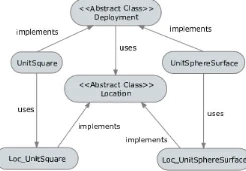
Figure 2 shows a simplified UML diagram of the ‘physical deployment’ component including two abstract classes (i.e.,
LocationandDeployment) and two implementations of each.
Figure 2: Physical deployment (topology) models
TheLocationclass describes abstract properties of a physi-cal location of a sensor node when deployed in a particular
region. Any sub-class ofLocationmust implement a method
to determine if two sensors are within a given communica-tion range or not. How the communicacommunica-tion range is defined depends entirely on the implementation.
The Deployment class contains attributes and methods of an object that represents a WSN deployment. The default constructor takes two parameters: the network size, and the communication range. The most important method in this abstract class generates a single node’s location. It is an ab-stract method, which must be implemented by sub-classes. Repeatedly calling this method generates the locations of all nodes. We assume that node locations remain static throughout the simulation, and that all nodes have homo-geneous communication range. Another important method is used to determine wireless connectivity in the network. This method is non-abstract, and provides a default imple-mentation to determine wireless connectivity. Basically, it loops through every possible node pair, and checks if they are within communication range of each other or not. A sub-class can override this default method, if desired. For example, execution speed may be improved by exploiting specific characteristics of a deployment (e.g., regular grid layout).
We implement two examples of deployment types. The first type assumes that sensor nodes are scattered uniformly at random within a unit square; this is a common model when studying WSNs [4]. One issue with this type of deployment isboundary effects: nodes near edges and corners have fewer wireless neighbors than other nodes. Thus, after the key es-tablishment phase, these nodes are more likely to be isolated from the network. This leads to discrepancies between ana-lytical results and simulation results, even when the network has 1,000 nodes or more. (Section 8 discusses this issue in more detail). In order to avoid boundary effects, our second deployment type considers sensor nodes that are distributed uniformly at random on the surface of a unit sphere (e.g., to model a planetary deployment). Although this is not a realistic model for most practical WSNs, it can be useful when studying WSNs without the boundary effect.
In the following, we describe the two implementations of WSN deployment in our system.
4.2
Sub-classes
4.2.1
Unit Square Deployment
Location and Communication Range
Each location in a unit square is given byxand y
coordi-nates. To generate a random location with uniform distribu-tion, we use the default random number generator provided by Java Development Kit (JDK) 1.6 to set each coordinate to a random value between 0 and 1. The distance between two nodes is evaluated as the Euclidean distance between their locations.
To reduce the computation time for wireless neighbor dis-covery, our implementation sorts the locations of all nodes
according to their x coordinate. This technique
substan-tially reduces the number of node pairs that must be con-sidered when determining wireless connectivity. This simple optimization significantly improves the execution time (e.g., 10-100 times faster than a brute force approach), especially when the WSN is very large (e.g., up to 10,000 nodes).
Determining Communication Range
Using the default constructor, one can generate a WSN physical deployment given a network size and a
communica-tion range. However, in some cases, it is more desirable to generate a network deployment given a network size and a specified average node density.
Analytically, we have derived a formula for the relationship between network size, average density, and communication
range. Specifically, ifnnodes with communication ranger
(0 < r <1) are distributed uniformly at random within a
unit square, then the average network densitynwis:
nw= (n−1)·(π·r2− 8 3·r 3+1 2·r 4) (1)
With this model, the simulation user can specify eitherthe
communication range or the network density for a given WSN size; the other value is computed automatically by the simulator.
4.2.2
Unit Sphere Surface Deployment
Location and Communication Range
In the unit sphere model, each point is represented by three
Cartesian coordinates (x, y, z). We employ Marsaglia’s
method [7] to generate random points on the unit sphere’s surface with a uniform distribution. The distance between two points is computed as the great-circle distance between them (i.e., path along the surface, not through the interior).
Determining Communication Range
We have also analytically determined the relationship be-tween network size, communication range, and network
den-sity in the unit sphere model. Given n sensor nodes
dis-tributed uniformly at random on a unit sphere’s surface, if
the desired average density is nw, then the communication
rangeris given by:
r=acos(1−2·nw
n−1) (2)
5.
KEY ESTABLISHMENT AND NODE
CAP-TURE MODEL COMPONENTS
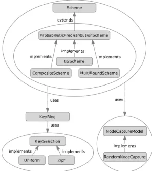
This section discusses the ‘key establishment’ and ‘node cap-ture model’ components, as illustrated in Figure 3.
5.1
Key Establishment Scheme
ClassSchemedefines the abstract design of an object
repre-senting a generic key establishment scheme. Examples of the abstract methods are a function to determine if two nodes share a key, a function to return the status (compromised or not) of a secure link, and a function to compute the pro-portion of compromised links in the network.
There are different categories of key establishment schemes, based on how they work. However, we focus only on
proba-bilistic key pre-distribution approaches.
ProbabilisticPredis-tributionScheme is an abstract class that extends Scheme, specifying additional methods of a generic probabilistic key
pre-distribution scheme, such as key ring generation. A
sub-component that facilitates key ring manipulation is de-scribed in Section 5.2.
We have fully implemented three schemes for probabilistic
key pre-distribution: EG,q-composite, and our own
multi-round scheme. The multi-multi-round scheme is our ongoing re-search and due to the nature of this paper, we do not go into the details of this scheme.
Figure 3: Key establishment and node capture
5.2
Key Ring and Key Selection
The key ring sub-component provides a method to construct a random key ring given the key pool size. Normally, a fixed number of keys are drawn uniformly at random from the key pool to create a key ring. Nevertheless, one may be interested in how different key selection methods influ-ence the performance of a particular probabilistic key pre-distribution scheme (e.g., heterogeneous key ring sizes, non-uniform key selection).
ClassKeyRingcan use any implementation of the abstract
classKeySelection to choose keys from the key pool when
forming a key ring. We have implemented two key selection methods: keys can be chosen with Uniform or Zipf
distri-butions. Additionally, the classKeyRingprovides a set of
functions for basic key ring manipulations, including union, intersection, and set membership operations.
5.3
Node Capture Model
The abstract classNodeCaptureModeldefines a method that
returns a set of captured nodes. Currently, we provide one
simple model, class RandomNodeCapture, which selects x
captured nodes (wherexis the input parameter) uniformly
at random from the set of all sensor nodes.
6.
NETWORK ANALYSIS COMPONENT
In this section, we describe the most essential analysis func-tions provided by the ‘network analysis’ component.
6.1
Connectivity
Connected components
We provide a function to find all connected components and
their sizes by doingbreadth-first search on a wireless trust
graph. From our observations, in many cases, when the net-work is disconnected only a few nodes around the boundaries and corners are isolated from the rest. In other words, de-spite the fact that the network is disconnected, the largest
connected component consists of most of the nodes. Sim-ply saying a network is connected or disconnected may not provide enough information when analyzing the connectiv-ity. For this reason, we compute and report all connected components.
Network connectivity
To determine if the network is connected or not, we provide a simple function that compares the size of the largest con-nected component to the network size. If they are equal, then the network is connected. Otherwise, the network is disconnected.
Coverage area
In some applications, it is useful to know the geographic area covered by a set of sensor nodes that are connected to each other. We provide a function to estimate the coverage area of one or more connected nodes.
Path length distribution
Another useful way of analyzing WSN connectivity is to measure the average path length between nodes. This metric provides an indication of the average power consumption for WSN communication. We provide a function implementing Floyd’s algorithm (all pairs shortest paths) on the wireless trust graph. It computes all paths, and then returns the distribution of the path length between every pair of nodes.
6.2
Key Ring Size and Key Usage
Initial key ring size
The key ring size is important in probabilistic key pre-distribution schemes. Large key rings improve the chances of connectiv-ity, but they also require more memory in sensor nodes, and increase the risk of link compromise when a node is cap-tured. Often one needs to estimate how many keys should be assigned to each sensor node so that there is a high prob-ability that the deployed WSN is connected. We provide a small program in the data collector package to determine
this value via simulation. It performs binary searchto find
the smallest initial key ring size so that the deployed WSN
is connected with high probability (i.e., at least itimes out
ofjsimulation runs, whereiandjare specified values for a
given network topology and key pool size).
Key usage
In most probabilistic key pre-distribution schemes, the as-signed keys from the key pool are rather sparsely used. We provide a function to examine the key usage distribution, particularly, how many keys are used once, twice, and so on. This usage distribution affects resilience to node capture.
Number of compromised keys
To study how many keys from the key pool are obtained by
an adversary who capturesxnodes (using a particular node
capture model), we provide a function that reports all the compromised keys.
6.3
Other Analysis Functions
In addition to the functions mentioned above, other useful analyses compute the distribution of wireless neighbors, the distribution of trust neighbors, the proportion of compro-mised links, and the probability that a link is comprocompro-mised if multi-path key reinforcement technique [3] is applied.
(a) A network with 10 nodes (b) A network with 1,000 nodes
Figure 4: Screenshots of GUI for WSN simulation tool
For almost every analysis function on a single WSN, there is a corresponding program in the data collector package to calculate the average result from a user-specified number of simulation replications.
7.
GUI COMPONENT
Figure 4 shows example screen shots of the graphical user interface of our simulation tool. Figure 4(a) shows a small 10-node WSN, while Figure 4(b) shows a large 1000-node WSN. In both examples, the rightmost pane shows the WSN layout, while the left side of the interface shows input pa-rameters and output results from the simulation.
There are two main control tabs on the top left of the GUI
windows: Simulation and Theory. The Theory tab allows
the user to study the analytical results of random graph theory, probability of key sharing, and so on with different parameters for comparison with the simulation results. We
concentrate here on the other main tab,Simulation. Under
Simulation, there are three sub-tabs that let the user enter simulation parameters, customize visualization, as well as select and view statistics and graphs based on the simulation results.
One parameter that the user needs to specify is the number of simulation replications. This parameter (default value is 1) can be changed in the data field next to the ‘Run simulation’ button in Figure 4. Once this button is hit, a WSN is simulated a number of times as stated by the users. When the simulation is done, the result appears on the text area beneath the ‘Run simulation’ button. Specifically, this text area summarizes the simulation parameters and pro-vides the simulation results including the average number of trust neighbors, the network connectivity, connected com-ponents, the number of compromised keys, the fraction of compromised links, running time, and so on.
The rightmost portion of the GUI in Figure 4 shows the
net-work visualization from themost recentsimulation run. In
the current system, we only provide the visualization for the unit square deployment model. We have no 3D visualization support for the spherical model.
Using the GUI to study WSNs, the user first needs to spec-ify parameters for simulation. Once the network has been simulated, network visualization can be customized to show different information. Furthermore, the user can examine the detailed (text-based) summary report from the simula-tion, or view the graphs generated from the simulation data. The following paragraphs elaborate on these steps.
Setting simulation parameters
To simulate a WSN, the user needs to select parameters for network topology, key establishment scheme, and (optional) node capture model. Besides, the user has to specify which analysis routines should be included in the simulation (for efficiency reasons), and the number of simulation replica-tions.
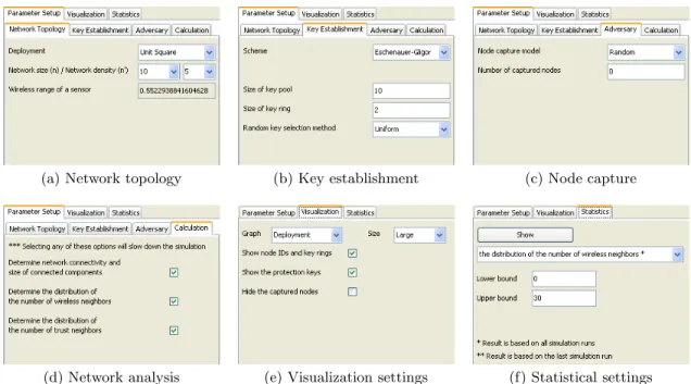
Figure 5 shows some of the menu selections and parameter controls for the user. Most simulation parameters can be set manually or chosen using drop-down menus and check boxes.
Inside theNetwork topologytab (Figure 5(a)), the user can
select the deployment type, and then set the network size and either communication range or network density. The data fields for network size and density are drop-down lists that consist of pre-defined common values. The text boxes are also editable so that the user can define any value they choose. As mentioned in Section 4.2, the communication range and the desired network density are related. Assuming that the user has chosen a network size and deployment type, whenever the desired density or the communication range is changed, the other setting is automatically calculated and updated accordingly.
From theKey Establishmenttab (Figure 5(b)), the user can
choose key establishment scheme, key pool size, key ring size, and key selection method.
TheAdversarytab (Figure 5(c)) specifies the node capture model (only one model currently) and the number of cap-tured nodes. The default value is 0, which means there is no adversary in the simulated WSN.
(a) Network topology (b) Key establishment (c) Node capture
(d) Network analysis (e) Visualization settings (f) Statistical settings
Figure 5: Setting simulation parameters
TheCalculation tab (Figure 5(d)) allows the user to spec-ify which network analysis functions are desired. There are some computationally expensive routines in the analysis of simulated WSNs which can be deactivated, avoiding extra overhead when simulating WSNs if the user is not inter-ested in those analyses. By default, all of these options are selected.
Customizing visualization
Figure 5(e) shows the ‘Visualization’ tab with various set-tings for customization. The drop-down list of graph types lets the user see different information about sensor nodes.
The available options arewireless range (the circular
com-munication range of each sensor node),wireless connectivity
(nodes that can communicate directly with each other), the
key graph(nodes that share at least one key), and the wire-less trust graph(secure connectivity).
To improve the clarity of the visualization, the user can se-lect one of the three sizes: ‘Small’, ‘Medium’, or ‘Large’. This setting scales the font size used, as well as the size of the dots and lines used to illustrate the WSN. For a large network, the visualization looks better with ‘Small’, and vice versa. The user also has an option to show or hide the node IDs, key rings, and protection keys of secure links, as well as the captured nodes and their attached compromised links. The network visualization shown in Figure 4a is a wireless trust graph of 10 sensor nodes. In this example, the key establishment scheme is EG, and each node is assigned two keys chosen randomly from a key pool of 10 keys. It is assumed that one node is captured by the adversary. In the visualization, the black dot indicates the captured node, while the red dots represent the other (uncaptured) nodes. For each node, we can see its ID followed by the IDs of keys that it has. In this example, node 3 is captured, and thus the adversary has keys 1 and 3. There is one compromised link
in the network, which is shown by the dashed line between nodes 3 and 6. The links that remain secure are shown with solid lines.
Graphical results
Figure 5(f) shows the options available under theStatistics
tab. In this tab, the user can choose to see the distribu-tion of the number of wireless neighbors or trust neighbors, and the distribution of path lengths based on the simulation result. The simulation data is fed into gnuplot to generate graphs, which are then presented to the user. Figure 6 shows an example diagram of the distribution of path length in a simulated WSN.
Figure 6: A diagram showing the distribution of path length in the simulated WSN
8.
APPLICATIONS AND SIMULATION
RE-SULTS
This section presents selected simulation results to demon-strate the functionality and value of our simulation tool for secure WSNs. First, we validate the theoretical results of network connectivity and link compromise probability in
the EG and q-composite schemes. Next, we examine the
boundary effects on network connectivity by i) comparing the predictions and experimental results of key ring size and
ii) investigating the difference of the distribution of node de-gree in random and wireless trust graphs. Finally, we use the simulator to study if the boundary effects become less noticeable in larger networks.
8.1
Simulation model validation
Network connectivity
Security analysis of EG protocol and its extension,q-composite
scheme, relies on modeling the key pre-distribution by a ran-dom graph. As the first application of the tool, we exam-ine the validity of this assumption. Assume that we want to deploy a network of 1,000 nodes in which the nodes are scattered uniformly at random on the unit sphere with an
average densitynw= 30 nodes. The desired connectivity is
99.9% and the key pool sizeN is 100,000.
According to random graph theory, a network of 1,000 nodes should be connected 99.9% of the time if the expected node
degree nt exceeds 13.8. Let ¯p be the probability that two
random key rings can be used to establish a pair-wise key. To satisfynt > 13.8 fornw = 30, wherent =nw·p¯, the
initial key ring size mmust be chosen such that ¯p > 13.8 30 .
For a key pool size N = 100,000, using the equations in
Section 2.2, we require m = 249 in the EG scheme, and
m= 394 for theq-composite scheme whenq= 2.
We ran the simulation experiments using these theoretical
key ring sizes for EG andq-composite schemes on the unit
sphere. The result shows that the network is connected 9,992 times out of 10,000 simulation runs for the EG scheme, and
9,994 times out of 10,000 simulation runs for theq-composite
scheme. These results confirm the mathematical analysis. The distribution of node degree is also very similar to that in a random graph.
Resilience against node capture attack
In the second set of simulation experiments, we verify the theoretical results of the effect of node capture attack. Re-call that the adversary can obtain all keys stored in captured nodes’ memory, allowing to compromise other secure links
with a non-zero probability1. Assume that we want to
com-pare the resilience against node capture attack in the EG
and q-composite schemes when q = 2 and q = 3. By a
similar derivation procedure of key ring size, we estimate
m= 502 for q-composite scheme when q = 3 to achieve a
connectivity of 99.9%. Using the same parameter settings for network topology, the simulation results are obtained and then compared with theoretical predictions in Figure 7. The results generated from our simulator are consistent with the
expected link compromise probability. That is,q-composite
scheme provides better resilience under small-scale node cap-ture attacks; however, its security weakens as the number of
captured nodes increases2.
8.2
Boundary effects
To study boundary effects, we repeated the previous exper-iments with the same parameter settings on the unit square deployment model. To approximate the initial key ring size
1The derivation and exact formulas of link compromise
prob-ability in the EG andq-composite schemes are available in [5]
and [3], respectively.
2Chanet al. explained this trade-off in [3].
0 0.2 0.4 0.6 0.8 1 0 100 200 300 400 500 600 700 800
Pr[a secure link is compromised]
Number of captured nodes EG (theory) EG (simulation) 2-composite (theory) 2-composite (simulation) 3-composite (theory) 3-composite (simulation)
Figure 7: Comparison of the resilience against node capture attack in the EG and q-composite schemes whenq= 2 and q= 3
for the connectivity of 99.9% using our tool, we perform
binary search for the smallest m such that the simulated
WSN is connected at least 9,990 times out of 10,000 sim-ulation runs (i.e., the connectivity is roughly 99.9%). The simulation results indicate that the EG scheme requires at
least 392 keys, while the q-composite scheme requires 537
keys.
The simulation results differ significantly from the theoret-ical results. Much larger key ring sizes (about 50% larger) are required for a desired connectivity of 99.9%. These dis-crepancies can be explained by:
• the small network size (1,000) compared to the
asymp-totic random graph theory result, and
• the existence of nodes around the boundaries and
cor-ners (these nodes have much lower chance to establish secure links with others because they have fewer wire-less neighbors).
8.3
Node degree
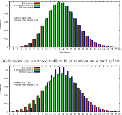
As mentioned earlier in the validation of network connec-tivity on the unit sphere, the distribution of node degree is very similar to that in a random graph. Figure 8a presents the comparison of this distribution, showing that they are very close. This is because in random graph and on sphere, virtually there is no boundary.
To investigate the influence of boundary effects on WSN connectivity, we run another set of simulation experiments to compare the node degree distribution in random graph to
those for the wireless trust graphs with EG orq-composite
scheme.
Recall that a random graph of 1,000 vertices is connected with 99.9% if the average node degree is 13.8; thus, the edge probability is ˆp= 13.8
999. The probability that a vertex has
a degree equal to dis n−1
d
!
·pˆd·(1−pˆ)n−1−dwhere
n is the number of vertices and hence equal to 1,000. This
equation allows us to find the distribution of node degree in a random graph of 1,000 vertices and the edge probability equal to 13.8
999.
Also, the mathematical analysis of EG andq-composite (q=
and 394, respectively, in order to ensure the expected node degree exceeds 13.8, making the deployed networks con-nected 99.9% of the time. We run the simulation 10,000 times using the theoretical initial key ring size with the cor-responding key establishment scheme to find the distribution of node degree.
Figure 8b compares the distribution of node degree in
ran-dom graph and the simulation results with both EG andq
-composite schemes on the wireless trust graph. Even though the average node degree in all three cases is approximately 13.8, the node degree distributions in the wireless trust graphs differ from that for the random graph. In particular, the wireless trust graphs have more nodes with low degree. The high number of low-degree nodes in the wireless trust graph indicates that nodes near the edges and corners are disad-vantaged in terms of secure connectivity.
8.4
Network size
In the last set of simulation experiments, we want to com-pare the theoretical initial key ring size with the actual key ring size in a larger network when the deployment region is a unit square. Specifically, the network size is 2,000, the av-erage density is 30, the key pool is 100,000 and the desired connectivity is 99.9%. The theoretical initial key ring size for EG scheme under this parameter set up is 287. The sim-ulation result suggests that the initial key ring size should be at least 397 for a connectivity of 99.9%. In the 2000-node case, the difference between the theoretical and simulation results is 38.4%, which is much lower than the 57.4% error for the 1000-node case. When the network size increases, the accuracy of the (asymptotic) random graph theory re-sult improves, but the estimation error is still noticeable
even whenn= 10,000 nodes.
In summary, the boundary effects have a significant impact on network connectivity. Although the estimation of initial key ring size is more accurate as the network size grows, it is still far from the actual value even if the network size is large. Therefore, studying the network connectivity for practical WSNs should consider boundary effects.
9.
CONCLUSION
This paper has presented an extensible simulator for the study of secure WSNs. We have found the simulator use-ful in the study of network connectivity, and demonstrated some discrepancies from the results predicted by random graph theory. For future work, we are planning to imple-ment adaptive node capture models and study their effect on the resilience of WSNs.
Acknowledgments
The authors thank the VALUETOOLS 2009 reviewers for their encouraging feedback on the initial version of this pa-per. Financial support for this research was provided by iCORE (Informatics Circle of Research Excellence) and NSERC (Natural Sciences and Engineering Research Council).
10.
REFERENCES
[1] Carey Williamson’s software page.
http://www.cpsc.ucalgary.ca/∼carey/software.html. [2] gnuplot.http://www.gnuplot.info. 0 0.02 0.04 0.06 0.08 0.1 1 2 3 4 5 6 7 8 9 10 11 12 13 14 15 16 17 18 19 20 21 22 23 24 25 26 27 28+ Probability Node degree Network size: 1000
Average node degree: 13.8 EG scheme q-composite scheme Random graph
(a) Sensors are scattered uniformly at randomon a unit sphere
0 0.02 0.04 0.06 0.08 0.1 1 2 3 4 5 6 7 8 9 10 11 12 13 14 15 16 17 18 19 20 21 22 23 24 25 26 27 28+ Probability Node degree Network size: 1000
Average node degree: 13.8 EG scheme q-composite scheme Random graph
(b) Sensors are scattered uniformly at randomin a unit square
Figure 8: Comparison of the node degree distribu-tion in random graph and in wireless trust graph with EG orq-composite key establishment
[3] H. Chan, A. Perrig, and D. Song. Random key predistribution schemes for sensor networks. In
Security and Privacy, 2003. Proceedings. 2003 Symposium on, pages 197–213, May 2003.
[4] R. Di Pietro, L. V. Mancini, A. Mei, A. Panconesi, and J. Radhakrishnan. Redoubtable sensor networks.
ACM Trans. Inf. Syst. Secur., 11(3):1–22, 2008. [5] L. Eschenauer and V. D. Gligor. A key-management
scheme for distributed sensor networks. InCCS ’02:
Proceedings of the 9th ACM conference on Computer and communications security, pages 41–47, New York, NY, USA, 2002. ACM.
[6] Internet Engineering Task Force. Diffie-hellman key agreement method.
http://tools.ietf.org/html/rfc2631.
[7] G. Marsaglia. Choosing a point from the surface of a
sphere.The Annals of Mathematical Statistics,
43:645–646, 1972.
[8] B. C. Neuman and T. Ts’o. Kerberos: an authentication service for computer networks.
Communications Magazine, IEEE, 32(9):33–38, Sep 1994.
[9] ns-2.http://www.isi.edu/nsnam/ns.
[10] J. Spencer.The Strange Logic of Random Graphs.
Springer-Verlag, 2000.
[11] O. Yagan and A. Makowski. On the random graph induced by a random key predistribution scheme
under full visibility. InInformation Theory, 2008.
ISIT 2008. IEEE International Symposium on, pages 544–548, July 2008.