Simulations and Modeling of Intermediate
Luminosity Optical Transients and Supernova
Impostors
Amit Kashi1 ID*
1 Department of Physics, Ariel University, Ariel, POB 3, 40700, Israel
* Correspondence:[email protected]; Tel.: +972-3-914-3046 ;http://www.ariel.ac.il/sites/amitkashi
Version June 25, 2018 submitted to
Abstract:Intermediate-luminosity-optical-transients (ILOTs) are stellar outbursts with luminosity
1
between those of classical novae and supernovae. They are divided into a number of sub-groups
2
depending on the erupting progenitor and the properties of the eruption. Many of the ILOTs sit on
3
the slanted Optical Transient Stripe (OTS) in the Energy-Time Diagram (ETD) that shows their total
4
energy vs. duration of their eruption. We describe the different kinds of ILOTs that populate the
5
OTS and other parts of the ETD. We also stand on similarities between Planetary Nebulae (PN) to
6
ILOTs, and suggest that some PNe were formed in an ILOT event. The high energy part of the OTS is
7
reserved to the supernova impostors – giant eruption of very massive stars. We show results of 3D
8
hydrodynamical simulations of supernova impostors that expose the mechanism behind these giant
9
eruptions, and present new models for recent ILOTs. We stand on the connection between different
10
kinds of ILOTs, and suggest that they are powered by a similar source of energy – gravitational
11
energy released by mass transfer.
12
Keywords:stellar evolution; late stage stellar evolution; binarity, transients, planetary nebulae
13
1. Introduction 14
Intermediate luminosity optical transients (ILOTs) are exotic transients which lies in between
15
the luminosities of novae and supernovae (SN). The group consists of many different astronomical
16
eruptions that at first appear to look different from one another, but found to have shared properties.
17
The different types of ILOTs are described in section2. The ILOTs we discuss in this paper and many
18
more are classified according to their total energy and eruption timescale (see section3) using a tool
19
named the energy-time diagram (ETD; seehttp://phsites.technion.ac.il/soker/ilot-club/). Most ILOTs
20
reside on the optical transient stripe (OTS) on the ETD, that gives us information about the power
21
involved in the eruption and its magnitude. A recent version of the ETD can be found in [14] and in
22
[24] published in the present special issue.
23
2. Types of ILOTs 24
The literature in recent years has been far from consistent in referring to transient events. Since
25
many ILOTs are being discovered, time has arrived for everyone to converge on one naming scheme
26
that will eliminate any ambiguity. In [12] we picked up the gauntlet and suggested a complete set of
27
names for the new types of transients. Since then, there have been developments in the field and new
28
types have been suggested. We therefore hereby update the classification scheme of ILOTs.
29
A. Type I ILOTs. Type I ILOTs is the term for the combined three groups listed below: ILRT,
30
LRN and LBV giant eruptions. These events share many common physical processes, in particular
31
being powered by gravitational energy released in a high-accretion rate event, according to the
32
high-accretion-powered ILOT (HAPI) model, discussed below. The condition for an ILOT to be
33
classified as type I is that the observing direction is such that the ILOT is not obscured from the
34
observer by an optically thick medium.
35
1. ILRT: Intermediate-Luminous Red Transients. Events involving evolved stars, such as
36
Asymptotic Giant Branch (AGB) stars and Extreme Asymptotic Giant Branch (ExAGB) stars,
37
and similar objects, e.g., Red Giant Branch (RGB) stars. The scenario which leads to theses events
38
is most probably a companion which accretes mass and the gravitational energy of the accreted
39
mass supplies the energy of the eruption. Examples include NGC 300 OT, SN 2008S, M31LRN
40
2015 (note the self-contradiction in the names of the last two transients).
41
2. LBV giant eruptions and SN Impostors. Giant eruptions of Luminous Blue Variables (LBVs).
42
Note that conventional S Dor eruptions are not included. These eruptions are the most energetic
43
ones among ILOTs, and the energy released in one or a sequence of those eruptions can reach
44
1049 erg and possibly more. Examples include the 1837–1856 Great Eruption of η Car, the 45
pre-explosion eruptions of SN 2009ip. ILRTs are the low mass relatives of LBV giant eruptions.
46
3. LRN or RT: Luminous Red Novae or Red Transients or Merger-bursts. These are powered by
47
a full merger of two stars. The process of destruction of the less dense star onto the denser
48
star releases gravitational energy that powers the transient. Examples include V838 Mon and
49
V1309 Sco.
50
B. Type II ILOTs.Type II ILOTs is the name of a new type of binary-powered ILOTs [13]. The
51
event may be similar to Type I ILOTs (type I), but different in the orientation of the observer, whose
52
line of sight crosses a thick dust torus or shell that obscures a direct view of the binary system or the
53
photosphere of the merger product.
54
The scenario for a type I ILOT is based on a strong binary interaction. Such an interaction can
55
be a periastron passage similar to the Great Eruption ofηCarinae [11], or a terminal merger. The 56
interaction leads to an axisymmetrical mass ejection with a large departure from spherical symmetry,
57
much like the morphologies of many planetary nebulae (e.g., [2,4,15,18,23]).
58
The obscuring matter would be in most cases equatorial, and will contain most of the ejected
59
mass. Until this dust disperses the binary system will be obscured to the eyes of the observer in the
60
visible and IR bands. The type II ILOT is accompanied by some polar mass ejection that may also
61
forms dust. The polar dust and gas reprocess the radiation from the central source, hence allowing
62
the observation of the type II ILOT, which becomes much fainter. A possible example is the outburst
63
observed from the red supergiant N6946-BH1 in 2009 [1].
64
C. Proposed scenarios for ILOTs. Other types of ILOTs have been suggested to exist, and
65
populate empty regions of the ETD.
66
1. Mergerburst between a planet and a brown dwarf (BD). In this process [3] the planet is shredded
67
into a disk, and the accretion lead to an outburst. The destruction of a component in a binary
68
system and transforming it to an accretion disk is an extreme case of mass transfer processes in
69
binary systems. The destruction of the planet before it hits the BD occurs because its average
70
density is lower than that of the BD. In that scenario it is required that the planet enters the tidal
71
radius. It may occur in a highly eccentric orbit that is perturbed. Once the planet is destructed, the
72
remnant of the merger behaves similarly to other ILOTs, such as V838 Mon, but on a shorter time
73
scale and with less energy. This process is a super Eddington process and these events occupy the
74
lower part of the OTS on the ETD.
75
2. Weak Outburst of a young stellar object (YSO). In [14] it was suggested that the unusual
76
outburst of the YSO ASASSN-15qi is an ILOT event, similar in many respects to V838 Mon,
77
but much fainter and of lower total energy. The erupting system was young, but unlike the
78
LRN, the secondary object that was tidally destroyed onto the primary main-sequence (MS) star
79
was suggested to be a Saturn-like planet rather than another low mass MS star. Such ILOTs are
80
unusual in the sense that they have low power and reside below the OTS.
81
3. ILOT which created a Planetary Nebulae (PN).In [25] we identified some intriguing similarities
82
between PNe and ILOTs: (a) a linear velocity-distance relation, (b) bipolar structure, (c), expansion
83
velocity of few×100km s−1, (d) total kinetic energy of≈1046–1049erg. We therefore suggest
that some PNe may have formed in an ILOT event lasting a few months (a short “lobe-forming”
85
event). The power source is similar, namely, mass accretion onto a MS companion from the AGB
86
(or ExAGB). Examples include the PN NGC 6302, and the pre-PNe OH231.8+4.2, M1-92, and
87
IRAS 22036+5306.
88
3. Common properties of ILOTs 89
In [10] we noticed that when scaling the time axis for ILOTs of the three kinds, an amazing
90
similarity in the light curve surfaces. From the peak or peaks of the lightcuve, the decline in the optical
91
bands with time is similar for almost four magnitudes. This could not be a coincidence, and a common
92
physical mechanism must have been involved in all ILOTs; one that resulted in a similar decline.
93
The high-accretion-powered ILOT (HAPI) model is a model that aims to focus on the shared
94
properties of many of the ILOTs. In its present state, the model accounts for the source and the amount
95
of energy involved in the events and for their timescales. The step of obtaining the exact decline rates
96
of the events has not yet been performed, and is currently under work.
97
The HAPI model is built on the premise that the luminosity of the ILOT comes from gravitational
98
energy of accreted mass that partially channeled to radiation. The radiation is eventually emitted in
99
the visible, possibly after scattering and/or absorption and re-emission.
100
To quantitatively obtain the power of the transients, we start by definingMaandRaas the mass 101
and radius (respectively) of star ‘a’, which accretes the mass. Star ‘b’ is the one that supplies the mass
102
to the accretion; it is possibly a destructed MS star, as in V838 Mon and V1309 Sco, or alternatively
103
an evolved star in an unstable phase of evolution that loses a huge amount of mass, as in the giant
104
eruptions ofη Car. The average total gravitational power is obtained by multiplying the average 105
accretion rate and the potential well of the accreting star
106
LG= GMa
˙
Ma
Ra . (1)
The accreted mass may form an accretion disk or a thick accretion belt around star ’a’. In the case of
107
a merger event this belt consists of the destructed star. The accretion time should be longer than the
108
viscosity time scale for the accreted mass to lose its angular momentum, so it can be actually accreted.
109
The viscosity timescale is scaled according to
110
tvisc' R 2 a
ν '73 α
0.1
−1H/Ra
0.1
−1C s/vφ
0.1 −1 Ra 5R 3/2 Ma 8M −1/2 days, (2)
whereHis the thickness of the disk,Csis the sound speed,αis the disk viscosity parameter,ν=αCsH 111
is the viscosity of the disk, andvφis the Keplerian velocity. We scale Ma andRa in equation (2)
112
according to the parameters of V838 Mon [28]. For these parameters, the ratio of viscosity to Keplerian
113
timescale isχ≡tvisc/tK'160. 114
The accreted mass is determined by the details of the binary interaction process, and varies for
115
different objects. We scale it byMacc=ηaMa. Based on the modeled systems (V838 Mon, V 1309 Sco, 116
ηCar) this mass fraction isηa.0.1 with a large variation. The value ofηa.0.1 can be understood as 117
follows. If the MS star collides with a star and tidally disrupts it, as in the model for V838 Mon [26,27],
118
the destructed star is likely be less massive than the accretorMacc< Mb.0.3Ma. In another possible 119
case an evolved star loses a huge amount of mass, but the accretor gains only a small fraction of the
120
ejected mass, as in the great eruption ofηCar. 121
The viscosity time scale gives an upper limit on the accretion rate
122
˙
Ma < ηaMa tvisc
'4ηa 0.1
α
0.1
H/Ra
0.1
Cs/vφ
0.1
Ra
5R
−3/2 M a
8M 3/2
The maximum gravitational power is therefore
123
LG <Lmax= GMa
˙
Ma Ra
'7.7×1041ηa 0.1
χ
160
−1 Ra
5R
−5/2 Ma
8M 5/2
erg s−1, (4)
where we replaced the parameters of the viscosity time scale with the ratio of viscosity to Keplerian
124
timeχ. 125
The upper bound on the OTS in the ETD is determined by equation (4), and describes a
126
supper-Eddington luminosity. The upper bound might be crossed if the accretion efficiency ηis 127
higher and/or the stellar parameters of the accreting star are different. For most of the ILOTs the
128
accretion efficiency is lower, hence they are located below the upper limit line, giving rise to the
129
relatively large width of the OTS. The uncertainty inηais large and may be even above unity, but 130
only in extreme cases. Therefore, one does not expect to find objects above the upper limit frequently.
131
We also note that the above estimate was performed with the expressions relevant for a thin disk
132
and a thick disk may need different treatment. A more accurate treatment requires hydrodynamic
133
simulations together with radiation transfer for obtaining the radiation emitted in each waveband.
134
4. Giant Eruptions in Very Massive Stars 135
As mentioned above, the most energetic ILOTs are the LBV giant eruptions. There is some
136
controversy about the identification of the stars which undergo giant eruption with LBVs, so for safety
137
we will refer to them as Very Massive Stars, or VMS.
138
In [9] we used the hydro codeFLASH[7] to model the response of a massive star to a high mass
139
loss episode. The hydro simulation started with the results of a run of a modified version of the 1D
140
stellar evolution codeMESA[19–22] in which we obtained a model of an evolved VMS. TheMESAstellar
141
model we obtained had properties similar to those of Eta Carinae, known for its giant eruptions in
142
the 19th century. We simulated hydrodynamically a giant eruption with the FLASH code using two
143
approaches: (1) Removing a layer from the star using energy from inner layers. (2) Extracting energy
144
from the core to outer layers that causes a spontaneous mass loss.
145
We found that the star developed a strong wind, powered by pulsation in the inner parts of the
146
star. The strong eruptive mass loss phase lasted for a few years, followed by centuries of continually
147
weakening mass loss. Figure (1) shows the resulted mass loss rate with time after the initiation of the
148
giant eruption. The three different lines indicate different simulations with a different amount of mass
149
removed from the VMS.
150
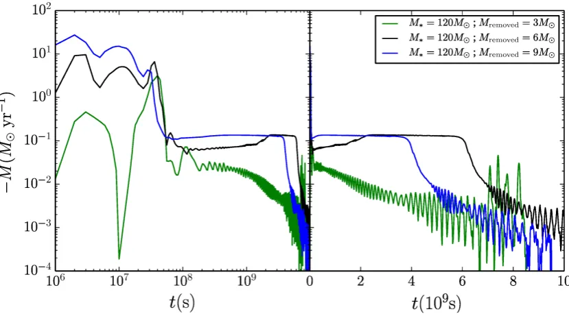
After about two centuries the mass loss rate of the star declined quite dramatically. The
151
explanation for this behavior is the change in the stellar structure as a response to the huge mass loss
152
in the giant eruption we simulated and the two hundred years of high mass loss rate that followed. At
153
a certain time the structure became such that the mechanism that accelerated the wind – non-adiabatic
154
κ-mechanism pulsations induced near the iron-bump – stopped being efficient. At that point the mass 155
loss rate decreased.
156
Observationally, the decline in mass loss rate we obtained was observed inηCar in the last two 157
decades. Variations in spectral properties of the star, especially near periastron passage and across
158
the spectroscopic event, taught us that this change-of-state has been happening [5,6,16]. However
159
the reason was at first unknown, until the simulations in [9] revealed the physical mechanism and
160
demonstrated its work.
161
In follow up simulations we were able to use super-high resolution to simulate a giant eruption
162
in 2D and 3D, for the first time. The purpose of doing so is to be able to investigate multidimensional
163
effects that cannot be completely or at all addressed otherwise: convection and mixing, rotation,
164
turbulence, hydrodynamical instabilities, meridional currents, tides, and especially multi-dimensional
165
pulsation. These effects are known to considerably influence the stellar properties, and therefore, we
166
expect them to have a significant impact on how a VMS recovers from an eruption.
Figure 1.Mass-loss rate as a function of time for runs using the 120MVMS model and approach 1 for initiating a giant eruption. The three different lines indicate different simulations with a different amount of mass removed from the VMS. Two of the runs (the blue and black lines) show a change of state in the mass loss rate about≈130 and≈190 years (respectively) after the giant eruption started, respectively. By that the simulations reproduce the decline in mass loss observed inηCar in the last years, (∼175 years after its great eruption), during which the mass loss rate has been declining by a factor of 2–4 (and possibly continues to decline).
Our 2D simulations produced an interesting result that could not have been obtained in 1D.
168
Assuming that the source of the giant eruption is the core, the eruption caused a Richtmyer-Meshkov
169
instability which propagated in the VMS during the days immediately following the giant eruption
170
(Figure2, left panel). That instability, in turn, caused strong dredging of species from the core to outer
171
layers. Nuclear processed material from the core moved to the outer layers and eventually was ejected
172
from the VMS. This may explain why the ejecta ofηCar is nitrogen rich. 173
Figure3shows the stellar properties as a function of time after the giant eruption. In the 3D
174
simulations, we found that the pulsations behaved much more chaotically and where much less
175
coherent than in the 1D simulations. The 3 spatial degrees of freedom in the 3D simulation engender
176
destructive interference of the pulsations (the chance of creating a constructive interference is low) that
177
damp the waves before they reach the surface and eject mass. As a result, the mass-loss rate obtained
178
after the eruption was smaller (Figure1), and during the period spanning the first few years after the
179
eruption the VMS reached an almost stable hydrostatic equilibrium.
180
In [11] we suggested that major LBV eruptions are triggered by binary interaction. The possible
181
most problematic example to be considered against our claim was P Cygni, as it was believed to be a
182
single star which underwent such an eruption. However [8] showed that even the eruption of P Cygni
183
presented evidence of binary interaction, printed in the varying time gaps between its consequentive
184
eruptions in the seventeenth century. Recently [17] used observations of P Cygni spanned over seven
185
decades, along with signal processing methods to identify a periodicity in the stellar luminosity. The
186
period they found is a possible indication for the presence of the companion suggested by [8] on
187
the basis of the theoretical arguments. This strengthened the conjecture that probably all major LBV
188
eruptions are triggered by interaction of a stellar companion.
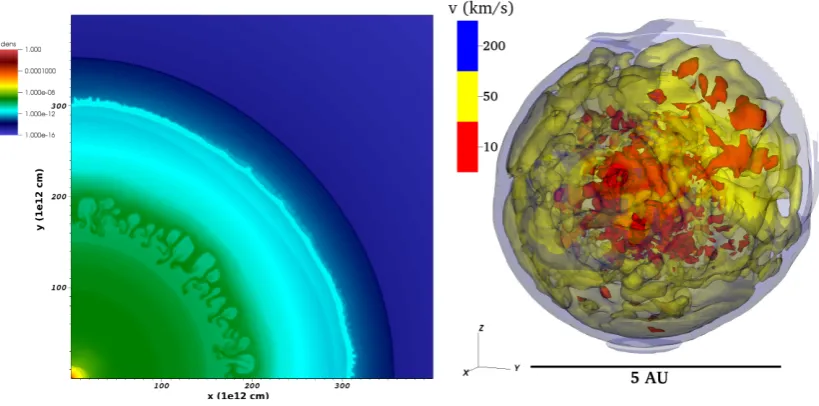
Figure 2. Left: A density map taken 5.8 days after the giant eruption. A layer experiencing the Richtmyer-Meshkov instability is seen atr'1.6–2.1×1014cm. This causes strong mixing of elements from the core to outer layers, which explains why the ejecta ofηCar is Nitrogen rich. Nuclear processed material from the core reaches the outer layers and is eventually ejected from the star.Right:Velocity 3D contours of the VMS and of the inner part of its clumpy wind 2.5 years after the giant eruption. The VMS has expended to≈500R, and is highly convective. Parts in the star are moving inward as a result of pulsation, while the outer layers move outward and create wind. The resultant wind was found to be slower, and the mass-loss rate was found to be smaller then that suggested by observations and by our 1D model. The reason for this change is the incoherency of the pulsations in 3D.
5. Summary 190
We discussed different types of ILOTs and categorized them in a manner that makes order in the
191
confused nomenclature in the field. We reviewed commonalities between these types and the HAPI
192
model that suggest they are all gravitationally powered. We put the spot light on the most massive
193
and energetic outburst that consist of the ILOTs group, the giant eruption in VMSs. The simulations
194
we showed explain the mechanism being the strong mass loss after the giant eruptions, and account
195
for the change of state in the mass loss more than 100 years after the eruption.
196
Acknowledgments: I thank Noam Soker and Amir Michaelis for helpful comments. Support from the the 197
Authority for Research & Development in Ariel University and the Rector of Ariel University is gratefully 198
acknowledged. This work used the Extreme Science and Engineering Discovery Environment (XSEDE) 199
TACC/Stampede2 at the service-provider through allocation TG-AST150018. This work was supported by 200
the Cy-Tera Project, which is co-funded by the European Regional Development Fund and the Republic of Cyprus 201
through the Research Promotion Foundation. 202
Abbreviations 203
The following abbreviations are used in this manuscript: 204
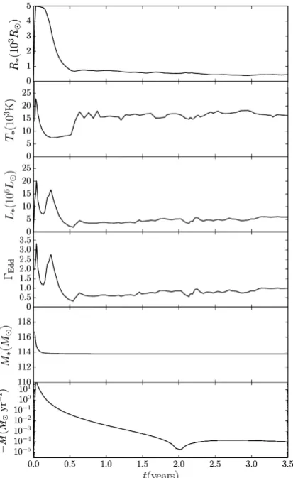
Figure 3.Results of one of our 3D simulations showing the recovery of a non-rotating VMS of 120M after removing an outer layer of 6Maccording to approach 2 (as a result of extracting energy from the core). From top to bottom, the panels show the stellar radius, effective temperature, luminosity, mass, Eddington ratio, and mass-loss rate. The temperature, radius and luminosity are calculated at optical depthτ=3. This figure can be compared to the right panel of figure 3 in [9], which shows the equivalent 1D simulation. In this 3D simulation, the first few years after the eruption bring the star to an almost stable hydrostatic equilibrium. The mass-loss rate is roughly two orders of magnitude smaller than that in the 1D simulation. Although the results of this preliminary work are still under study, they are probably due to the lower coherency of the pulsations in the 3D compared to the 1D simulation. The three spatial degrees of freedom engender destructive interference of the pulsations that damp the waves before they reach the surface and eject mass.
AGB Asymptotic Giant Branch
ASASSN All-Sky Automated Survey for Supernovae
BD Brown Dwarf
ETD Energy-Time Diagram
ExAGB Extreme Asymptotic Giant Branch HAPI High Accretion Powered ILOT
ILOT Intermediate Luminosity Optical Transient ILRT Intermediate Luminosity Red Transient LBV Luminous Blue Variable
LRN Luminous Red Nova
MESA Modules for Experiments in Stellar Astrophysics MS Main Sequence
OTS Optical Transient Stripe PN Planetary Nebulae
SN Supernova
References 207
1. Adams, S. M., Kochanek, C. S., Gerke, J. R., Stanek, K. Z., & Dai, X. 2017, MNRAS, 468, 4968 208
2. Balick, B. 1987, AJ, 94, 671 209
3. Bear, E., Kashi, A., & Soker, N. 2011, MNRAS, 416, 1965 210
4. Corradi, R. L. M., & Schwarz, H. E. 1995, A & A, 293, 871 211
5. Davidson, K., Ishibashi, K., Martin, J. C., & Humphreys, R. M. 2018, ApJ, 858, 109 212
6. Davidson, K., Martin, J., Humphreys, R. M., et al. 2005, AJ, 129, 900 213
7. Fryxell, B., Olson, K., Ricker, P., et al. 2000, ApJS, 131, 273 214
8. Kashi, A. 2010, MNRAS, 405, 1924 215
9. Kashi, A., Davidson, K., & Humphreys, R. M. 2016, ApJ, 817, 66 216
10. Kashi, A., Frankowski, A., & Soker, N. 2010, ApJL, 709, L11 217
11. Kashi, A., & Soker, N. 2010, ApJ, 723, 602 218
12. Kashi, A., & Soker, N. 2016, Research in Astronomy and Astrophysics, 16, 99 219
13. Kashi, A., & Soker, N. 2017a, MNRAS, 467, 3299 220
14. Kashi, A., & Soker, N. 2017b, MNRAS, 468, 4938 221
15. Manchado, A., Guerrero, M. A., Stanghellini, L., & Serra-Ricart, M. 1996, The IAC morphological catalog 222
of northern Galactic planetary nebulae (Publisher: La Laguna, Spain: Instituto de Astrofisica de Canarias 223
(IAC)), 1996, Foreword by Stuart R. Pottasch, ISBN: 8492180609 224
16. Mehner, A., Davidson, K., Humphreys, R. M., et al. 2015, A & A, 578, A122 225
17. Michaelis, A. M., Kashi, A., & Kochiashvili, N. 2018, New Astronomy, 65, 29 226
18. Parker, Q. A., Bojiˇci´c, I. S., & Frew, D. J. 2016, Journal of Physics Conference Series, 728, 032008 227
19. Paxton, B., Bildsten, L., Dotter, A., et al. 2011, ApJS, 192, 3 228
20. Paxton, B., Cantiello, M., Arras, P., et al. 2013, ApJS, 208, 4 229
21. Paxton, B., Marchant, P., Schwab, J., et al. 2015, ApJS, 220, 15 230
22. Paxton, B., Schwab, J., Bauer, E. B., et al. 2018, ApJS, 234, 34 231
23. Sahai, R., Morris, M. R., & Villar, G. G. 2011, AJ, 141, 134 232
24. Soker, N. 2018, Galaxies, 6, 58 233
25. Soker, N., & Kashi, A. 2012, ApJ, 746, 100 234
26. Soker, N., & Tylenda, R. 2006, MNRAS, 373, 733 235
27. Tylenda, R., & Soker, N. 2006, A & A, 451, 223 236