Article
Using Tandem-X Science Phase Observations to
Extract Glacial Topography
Sang-Hoon Hong 1, Shimon Wdowinski 2, Falk Amelung 3, Hyun-Cheol Kim 4,
Joong-Sun Won 5 and Sang-Wan Kim 6, *
1 Department of Geological Sciences, Pusan National University, Pusan, 46241, Korea;
2 Department of Earth & Environment, Florida International University, FL, 33199, U.S.A.;
3 Department of Marine Geosciences, University of Miami, FL, 33149, U.S.A.; [email protected]
4 Unit of Arctic Sea-Ice Prediction, Korea Polar Research Institute, Incheon, 21990, Korea; [email protected]
5 Department of Earth System Sciences, Yonsei University, Seoul, 03722, Korea; [email protected]
6 Department of Energy & Mineral Resources Engineering, Sejong University, Seoul, 05006 Korea;
* Correspondence: [email protected]; Tel.: +82-2-3408-3723
Abstract: Space-based Interferometric Synthetic Aperture Radar (InSAR) applications have been widely used to monitor the cryosphere over past decades. Because of temporal decorrelation, interferometric coherence often severely degrades on fast moving glaciers. In addition, higher sensitivity ambiguity occurs in large baseline configurations, which are needed for extracting topographic information over low relief areas such as the surface of a glacier. TerraSAR-X add-on for Digital Elevation Measurement (TanDEM-X) observations, which overcome the temporal decorrelation because of their simultaneous measurements by two satellite constellations, have used a short baseline sufficient for generation of excellent digital elevation models in most locations around the world. However, it remains difficult to estimate detailed topographic characteristics over low slope glacier surfaces because of the relatively less sensitive height ambiguity from the small baselines. In this study, we used the TanDEM-X pursuit monostatic mode with large baseline formation following a scientific phase timeline to develop highly sensitive topographic elevation models of the Petermann Glacier of Northwest Greenland. As expected, coherent interferometric phases (> 0.8) were well maintained over the glaciers despite their fast movement thanks to the nearly simultaneous TanDEM‐X measurements. The height ambiguity, which defined as the altitude difference correspondent to
2
phase change of flattened interferogram, of the dataset was 10.63 m, which is favorable for extracting topography in a low relief region. We validated the TanDEM‐X derived glacial topography by comparing it to the SAR/Interferometric radar altimeter observations acquired by CryoSat‐2 and the IceBridge Airborne Topographic Mapper laser altimeter measurements. Both observations showed very good correlation within a few meters of the offsets (‐12.5 – ‐3.1 m) with respect to the derived glacial topography. Because of highly sensitive ambiguity, we could successfully extract detailed geomorphological features on the glaciers. Routine TanDEM-X observations will be very useful to better understand the dynamics of glacial movements and topographic change.Keywords: TanDEM-X, digital elevation model, TanDEM-X Science Phase, radar interferometry, Petermann Glacier, ambiguity height
1. Introduction
In both Greenland and Antarctica, significant loss of glaciers play an important role as sensitive indicators and modulators of the global climate system interacting with the ocean and atmosphere
[1-3]. In Greenland, the calculated average ice mass loss over the entire ice sheet between 2002 and 2015 has been estimated as 238 gigatons per year (Gt/yr) [4-6]. Meehl et al. indicated that sea level would rise approximately 6 m (m) if Greenland’s ice sheet were to completely melt [7] and projected a sea level rise of between 0.5 and 1.5 m by 2100 [8,9]. Monitoring these rapid changes in polar regions is important in terms of evaluating the vulnerability of the cryosphere as well as for constraining regional and global climate change models. In glacier monitoring, precise topographic observations of glaciers have been an invaluable resource to evaluate glaciological mass balance affecting sea-level rise [10-15]. Howat el al. reported that rapid change of ice discharge in Greenland outlet glacier using satellite-derived surface elevation model [16]. High-resolution digital elevation models (DEMs) using unmanned aerial vehicle (UAV) was successfully utilized to assess calving dynamics at Greenland outlet glacier [17]. A review paper pointed out that the high-resolution DEMs can be very useful resources to describe ice sheet mass balance in Greenland [18]. Conventional TanDEM-X DEM were successfully used to calculate elevation change for glacier monitoring [19,20].
Although, however, the high-resolution DEMs is one of essential resources to understand mass balance in ice sheet, generation of precise DEMS in the cryosphere remains as a difficult task. The main obstacles in observing surface height of the cryosphere might be the inaccessibility due to the inhospitable conditions and the darkness of the polar night. Developments in remote-sensing techniques have aided in the successful development of DEMs over glacial surfaces to overcome these obstacles. Topographic information of glaciers has been measured using space-based radar and laser altimetry using satellites such as ERS-1/2, Envisat, ICESat and CryoSat-2. Although satellite altimetry observations can retrieve precise surface height of a glacier with a single observation, it is difficult to inspect the surface of glaciers in much detail because they provide limited measurements between orbits. Moreover, they often lose accuracy where the gradient of a slope significantly changes [21]. Despite the inhospitable conditions that restrict access to the cryosphere, airborne sensors such as those used during Operation IceBridge have been successfully used in previous campaigns. However, it is impossible to generate a precise DEM of the entire polar regions because of costs and access restrictions.
Near-global DEMs such as the Shuttle Radar Topographic Mission (SRTM) and Advanced Spaceborne Thermal Emission and Reflection Radiometer (ASTER) Global Digital Elevation Model (GDEM) have been released. While the GDEM utilizes stereo optical imagery, the SRTM data relies on single-pass InSAR observations. Both DEMs, particularly the SRTM DEM, are quite limited for use in cryospheric studies because the coverage of the SRTM DEM extends only from 56°S to 60°N and that of the GDEM extends from 83°N to 83°S. The vertical accuracy of these DEMs ranges from 6 to 16 m [22] and outdated topographic information might prevent accurate calculation of glacial characteristics. In addition, the spatial resolution of both DEMs is approximately 30 m, which is too coarse to investigate detailed features of a glacier.
multiple topographic observations has been reported [19,20]. Because, however, the calculated DEMs might not show detail topographic characteristics because of relatively large height of ambiguity. After the global TanDEM-X DEM mission, the TanDEM-X Science Phase mode was conducted temporarily from October, 2014, to December, 2015, over 15 months to experiment with special orbital configurations for scientific purposes [29]. A large perpendicular baseline and a very short or no temporal baseline from the TanDEM-X observations during the Science Phase is preferable to construct more accurate DEMs over low-relief areas such as intertidal or glacial surfaces [30].
In this study, we examined the feasibility of the TanDEM-X pursuit monostatic observation acquired during the TanDEM-X Science Phase to construct high-resolution and highly sensitive topographic elevation models that cannot be achieved using other conventional InSAR observations. The objective of this study is to evaluate of estimating more detailed topographic height variation along a low slope moving surface like a glacier rather than assess the accuracy of the constructed DEM in a single TanDEM-X Science Phase observation. The study area was selected as the Petermann Glacier’s low-gradient surface for developing more precise topographic information. First, the absolute topographic elevation model with an improved height of sensitivity by large perpendicular baseline formation was estimated using an InSAR technique. Then, an accuracy assessment was performed using existing DEMs such as the Greenland Ice Mapping Project (GIMP) DEM and global TanDEM-X DEM, CryoSat-2 radar altimeter observations (SAR/Interferometric mode (SARIn)) and IceBridge Airborne Topographic Mapper (ATM) laser altimeter measurements.
2. Materials and Methods 2.1. Study area
The study site was the Petermann Glacier which has attracted great attention from the impact of a 2010 calving event (Figure 1(a-c)). The Petermann Glacier is in Northwest Greenland (near 81° north) and connects the Greenland ice sheet to the Arctic Ocean (Figure 1(d)). The Petermann Glacier is approximately 70 km in length and 15 km in width with typical floating tongues and ice shelves of a low surface gradient [31]. The ice thickness changes from approximately 600 m at its grounding line to less than 100 m at its front [32]. The mass balance in Greenland has been studied extensively [14-18]. Noel Gourmelen indicated that elevation changes of Petermann glacier could be monitored conventional TanDEM-X observation [33]. Because of two calving events during August 2010 and July 2012, dramatic glacier loss of approximately 40% of the floating portion of the glacier has occurred and approximately 35 km of glacier retreat has been observed. Figure 1(a) is the Landsat-5 Thematic Mapper (TM) acquired on June 15,2009, and Figure 1(b) is the Landsat-8 Operational Land Imager (OLI) optic image captured on March 30, 2015. The glacier loss resulting from the calving events can be clearly monitored by both of the optic observations shown in Figure 1(a-b). However, both the velocity and thickness of the glacier have not significantly changed as a result of these two massive calving events [34]. Nevertheless, there is great concern of possible acceleration of glacial retreat or a calving event in one of the largest remaining floating ice shelves in the Northern Hemisphere.
2.2. Data
2.2.1. TerraSAR-X and TanDEM-X SAR
maintain coherence even on rapidly moving surfaces. The characteristics of the TerraSAR-X and TanDEM-X SAR are summarized in Table 1. To retrieve the topographic information for the entire Petermann Glacier area, two consecutive SAR observations were concatenated.
Figure 1. (a) Multi-spectral Landsat-5 TM optic image acquired on June 15, 2009, before the calving event that occurred during August 2010. (b) Landsat-8 OLI captured on March 30,2015, after both calving events of 2010 and 2012. The glacier loss in terminus areas is clearly detected through the two optic remotely-sensed observations. (c) TerraSAR-X SAR amplitude image on February 21,2015, over the Petermann Glacier in Northwest Greenland. (d) Location map of the Petermann Glacier showing the TerraSAR-X/TanDEM-X swath, marked by the black frame, used in this study.
Table 1. TerraSAR-X and TanDEM-X SAR data characteristics used in this study
Parameter TerraSAR-X/TanDEM-X
Acquisition date February 21, 2015
Carrier frequency X-band (9.6 GHz)
Wavelength 3.1 cm
Polarization HH
Incidence angle 35.28 / 35.33 degrees
Pulse repetition frequency 3700 Hz
ADC sampling rate 164.8 MHz
Azimuth pixel spacing 1.90 m
2.2.2. GIMP DEM and global TanDEM-X DEM
To calibrate and validate the constructed DEM, we collected the GIMP DEM and global TanDEM-X DEM. The GIMP DEM has been constructed by merging the ASTER GDEM [35] and SPOT-5 DEM of the SPOT-5 stereoscopic survey of Polar Ice. The Reference Images and Topographies (SPIRIT) program was used [36] for the peripheral ice sheet and the photo-enhanced Bamber (PEB) AVHRR DEM was utilized [37] for the interior ice sheet [38]. A comparison to the ICESat measurement shows 9.1 m of overall root mean square validation error (RMSE), 8.5 m over the ice-covered terrain, and 18.3 m in the ice-free high relief region. The GIMP DEM data is composed of 36 geotiff format tiles with a ESPG 3413 projection and an WGS84 ellipsoid [38].
In addition, the global TanDEM-X DEM was also used for accuracy assessment of the constructed DEM. Single-pass radar interferometry with a close flight formation of TerraSAR-X and TanDEM-X enables development of a world-wide DEM with 12-m horizontal resolution and 2-m relative height accuracy for flat terrain [23]. A comparison to Global Positioning System (GPS) observations shows that a small absolute vertical mean error for the global TanDEM-X DEM (< 0.20 m) and a small RMSE (< 1.4 m) [39]. We obtained 12-m resolution in the DEM over the Petermann Glacier through a science proposal from the TanDEM-X Science Coordination.
2.2.3. CryoSat-2 Radar Altimeter
CryoSat-2 is a radar altimetry satellite built by the European Space Agency (ESA) and its mission is dedicated to the monitoring of ice sheets on land and sea ice in the ocean. The orbit of CryoSat-2 has a 92° inclination and a 717-km altitude and covers nearly all of the polar regions (~88°N). The Synthetic Aperture Radar/Interferometric Radar Altimeter (SIRAL) altimeter in the Ku-band (13.575 GHz) provides an approximately 0.3 km by 1.5 km area along track and across track, which is a greatly reduced size of footprint compared to previous ESA altimeter missions such as ERS and the Envisat system (~10 km) [40,41]. Three operational modes of low resolution, SAR, and SARIn are available. The height accuracy of CryoSat-2 SAR has more than 4 m of bias at the steep margin of the ice sheet, and a 1.5-m bias in flat areas with slopes less than 0.2° [42,43]. A total of 22 CryoSat-2 SARIn mode observations from January 22, 2015 to March 21, 2015 were collected to validate the constructed DEM and convert the geodetic map projection into a polar stereographic projection (Table 2.).
2.2.4. IceBridge ATM Laser Altimeter
Table 2. Acquisition date of the CryoSat-2 and IceBridge ATM altimeter datasets
CryoSat-2 Radar Altimeter IceBridge ATM Laser Altimeter
Acquisition January 22, 2015 (D*) January 24, 2015 (D) May 5, 2015 12:35:55
Date January 26, 2015 (D) January 28, 2015 (D) May 5, 2015 12:45:06
January 30, 2015 (D) February 7, 2015 (A) May 5, 2015 12:50:02
February 9, 2015 (A) February 11, 2015 (A) May 5, 2015 12:56:20
February 13, 2015 (A) February 15, 2015 (A) May 5, 2015 13:06:14
February 18, 2015 (D) February 20, 2015 (D) May 5, 2015 14:38:29
February 22, 2015 (D) February 24, 2015 (D)
February 26, 2015 (D) February 28, 2015 (D)
March 8, 2015 (A) March 10, 2015 (A)
March 12, 2015 (A) March 14, 2015 (A)
March 19, 2015 (D) March 21, 2015 (D) *A: Ascending orbit, D: Descending orbit
2.3. Methods
2.3.1. Data processing
The InSAR application using consecutive TanDEM-X SAR observations is a well-known technique to construct precise DEMs [23]. However, two important steps are essential for the processing of InSAR pairs with a large geometric baseline. The first is applying common band filtering in the range direction to compensate for the geometric decorrelation because the large geometric baseline results in spectral decorrelation in range direction. The other is careful application of the unwrapping procedure. During the conventional TanDEM-X SAR interferometric processing under normal operation, the height of ambiguity ranging from 30 m to 45 m might not produce a severe interferometric phase aliasing at a steep slope area such as a high mountainous area. However, a small height of ambiguity because of a large perpendicular baseline can produce an undesirable interferometric phase aliasing even in low mountains. Although there is no interferometric phase aliasing in a low slope area such as a glacial surface, it might be useful to update existing topographic information by adding a differential interferometric phase.
We processed the TanDEM-X COSAR SLC acquisitions using the Gamma software package [47]. Precise coregistration at a sub-pixel scale is required to reduce the decorrelation effect during data processing [48]. Because a large geometric baseline results in wavenumber shifts in the range direction, common range spectral filtering should be applied [49]. Although the difference in the Doppler central frequency of -51.55 Hz (35.33 Hz in the TerraSAR-X image and -16.22 Hz in the TanDEM-X image) was not sufficiently large to result in severe Doppler decorrelation, we applied azimuth spectral common band filtering [50]. After common band filtering has been applied in both the range and azimuth directions, the flat Earth phase was removed from the raw interferogram. The phase ramp, which was determined by the baseline components of the two SAR sensor geometries, was subtracted. In the case that the systematic residual fringes remained, additional phase removal using fringe rate estimation by two-dimensional fast Fourier transform (FFT) should be applied. Multi-looking techniques of interferograms and adaptive phase filtering were applied to improve the signal-to-noise ratio (SNR) [51]. The multi-looking factor was chosen as 2 by 2; hence, the pixel spacing of the resampled interferogram doubled to 1.82 m and 3.80 m in the range and azimuth directions, respectively. Coherence is a quantitative value showing the amount of correlation between the two SAR observations. To evaluate the quality of the InSAR pair, we conducted a coherence analysis using a 5- 5-pixel window.
phase contained only the surface displacement between the two observations and possible topographic errors. The Minimum Cost Flow (MCF) algorithm was used for phase unwrapping of the differential interferometric phase [47]. The 0.9 of coherence threshold for masking decorrelated phases was used before the phase unwrapping process. The unwrapped phases were added to the simulated topographic phases from the GIMP DEM. To estimate the interferometric baseline, ground control points (GCPs) with terrain height information are required. Because it is very difficult to select the GCPs over moving glacial surfaces or snow/ice-covered areas, we utilized the GIMP DEM to select the GCPs. Before we selected the GCPs from the GIMP DEM, the GIMP DEM was converted into range-Doppler coordinates. The unwrapped phase was converted into a height map using the baseline geometry in the slant range geometry. Then, the final DEM using TanDEM-X Science Phase was constructed using a geocoding process.
3. Results
3.1. DEM construction
The filtered interferogram after the flat Earth phase removal is shown in Figure 2(a). Because of the very short temporal baseline of only 10 s, very high coherent interferometric phases were maintained over nearly the entire scene even on sea ice near the glacier terminus (the upper part of the interferogram). Very short wavelength of the fringes caused by the high sensitivity of the height ambiguity can be found in the bedrock region near the glacier margin, whereas a low fringe rate is shown on the glacier surface. Very detailed topographic characteristics of the glacier surface have been retrieved by the high sensitivity of the height ambiguity. Although phase unwrapping of the longer wavelength fringes on the relatively flat slope area was not a significant issue, the differential interferogram subtracted from simulated topographic phase of the GIMP DEM was calculated (Figure 2(b)). Note that a relatively high rate of fringe was sufficiently eliminated overall in the areas. It is interesting that the GIMP DEM can be successfully utilized for subtraction topographic phases even on rapidly moving surfaces.
Figure 2. (a) Filtered interferogram (February 21, 2015) after flat Earth phase removal showing topographic features on the glacier surface. Because of the high sensitivity of the height ambiguity, the remarkably detailed fringe pattern on the glacier surface and the very short wavelength of the fringes in the bedrock regions near the glacier were detected. (b) Differential interferometric phase scaled from
−
to
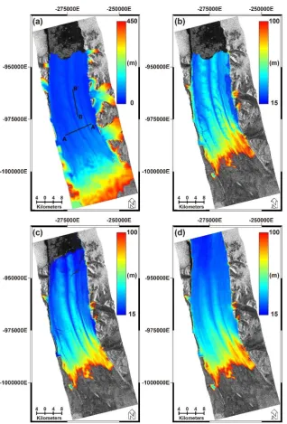
subtracted from the simulated topographic phase of the GIMP DEM. (c) Interferometric coherence ranges from 0 to 1 showing a very high coherence glacier surface except for the regions marked by red circles. This might have resulted from relatively faster glacier movement or a difference in glacial surface roughness.Figure 3(a) shows the constructed DEM scaled only from 0 to 450 m excluding the bedrock areas which have a higher elevation as we are interested in the topography of the glacier surface. The topographic height of the minor tributaries as well as the primary tributary of the Petermann Glacier has been successfully retrieved using the pursuit monostatic TanDEM-X pair with a large perpendicular baseline configuration. To impose the usefulness of the large perpendicular baseline in a low slope area, we also show the constructed DEM scaled from 15 to 100 m in Figure 3(b). The global TanDEM-X DEM and the GIMP DEM are shown in Figure 3(c) and (d), respectively, for visual inspection at the same scale. First, the constructed DEM shows the most detailed topographic variation over the glacier surface compared to that of other two DEMs. The 12 m of high spatial resolution of the global DEM also shows the detailed topographic surface of the glacier. However, the relatively more moderate to larger height of ambiguity ranges from 30 to 45 m providing less detailed topographic features compared to those of the derived DEM using the TanDEM-X Science Phase observation. The GIMP DEM does not have sufficient vertical accuracy to discriminate the detailed characteristics of the glacier surface.
Figure 3. (a) Constructed DEM scaled from 0 to 450 m excluding the bedrock regions that were not of interest in this study. The topographic information was successfully extracted using the pursuit monostatic TanDEM-X Science Phase mode. To impose the advantage of a large perpendicular baseline in a low slope area, the constructed DEMs of (b) the TanDEM-X Science Phase mode, (c) the global TanDEM-X DEM, and (d) the GIMP DEM, scaled from 15 to 100 m, are shown. Note that the derived DEM, thanks to large perpendicular baseline configuration in this study, shows much clearer topographic change along the glacier surface.
3.2. Validation using existing DEMs
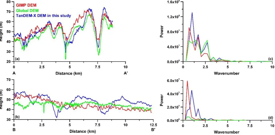
variation can be detected by comparing the DEMs. The constructed TanDEM-X DEM shows very detailed topographic changes over the glacier surface, whereas other two DEMs do not show very sensitive topographic information over the glacier. To investigate spatial details of each DEMs, a frequency analysis using fast fourier transform (FFT) was applied at each DEM profiles (Figure 4(c-d)). In the power spectrum of the profile A-A’, similar or slightly higher frequency of derived TanDEM-X DEM was detected. Higher frequency component of constructed DEM compared with other DEMs was calculated in the profile B-B’. Thus, the TanDEM-X DEM with small height of ambiguity reflected more detail topographic information which can be useful for monitoring ice volume over a glacier.
Figure 4. Surface profiles along the (a) A-A’ and (b) B-B’ traverse lines shown in Figure 3(a). The power spectrum (c and d) using frequency analysis on (a) A-A’ and (b) B-B’ was displayed. The red line is the profile of the GIMP DEM, the green line is from the global TanDEM-X DEM, and the blue one is based on the TanDEM-X Science Phase mode. The constructed TanDEM-X DEM shows very detailed surface characteristics, whereas the other two DEMs do not show much sensitive topographic variation along the B-B’ profile.
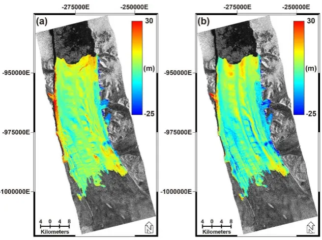
Figure 5. Difference map, scaled from -25 m to 30 m, of the topographic height between the constructed DEM and (a) the global TanDEM-X DEM and (b) GIMP DEM. These show that the constructed DEM provides much more detailed topographic surface information compared to that of the other DEMs.
The scatter plots between the constructed TanDEM-X DEM and the two other DEMs are shown in Figure 6 for validation points. The validation points were chosen at the same position where the CryoSat-2 observations are available. We assumed that there was only an offset between the two heights as Y = X + offset. They show a very good correlation of 0.998, and the offsets were calculated as -3.1 m and -7.0 m for the GIMP and Global DEM. Because the constructed DEM utilized the GIMP DEM as a reference height, a relatively smaller offset might have been estimated. Moreover, each DEM has a different height sensitivity level or vertical accuracy, which can be one of the reasons it is showing the offset difference.
Figure 6. Scatter plots between the constructed DEM and the other two DEMS of (a) the global TanDEM-X DEM and (b) the GIMP DEM. We assumed that there was only an offset between two
3.3. Validation with altimetry observations
We adjusted the CryoSat-2 and IceBridge ATM observations to fit the coverage of the TanDEM-X SAR acquisitions to validate the constructed DEM (Figure 7(a-b)). Much more CryoSat-2 altimetry measurements than ATM observations were collected. The trajectory of the three ATM observations flown along the glacier surface are shown in Figure 7(b).
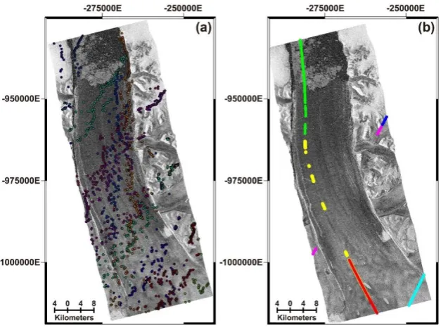
Figure 7. (a) The location of the CryoSat-2 altimetry measurements collected for two months from January 22, 2015 to March 19, 2015 as shown in Table 2 and the (b) IceBridge ATM observations acquired on May 5, 2015. Most of the ATM observations were collected along the path of the Petermann Glacier flow.
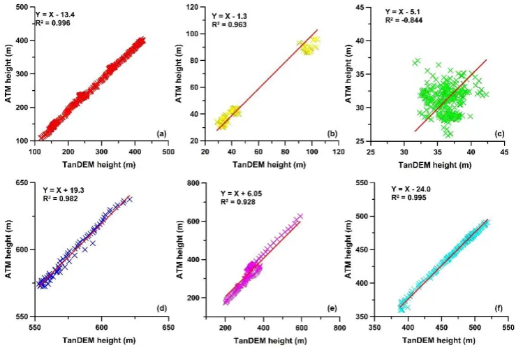
We show the scatter plots between the constructed TanDEM-X DEM and the two altimetry observations in the same manner as the comparison to the other DEMs (Figure 8). Before plotting, the suspicious CryoSat-2 observations around the rough and steep terrain area were set as outliers. The high correlation coefficients of the CryoSat-2 and ATM were 0.998 and 0.995, respectively. The calculated offset of the CryoSat-2 case was just -6.5 m, but -12.5 m of offset was found for the ATM observation, which is slightly larger than that of the CryoSat-2.
Y
=
X
+
offset
. They show a very good correlation coefficient, 2R
of 0.995, and the calculated offset of the CryoSat-2 and ATM altimetry observations were -6.5 m and -12.5 m, respectively.The scatter plots along the six ATM flight paths are shown in Figure 9 to examine the cause of the larger offset. We noticed that the larger offsets were found at both the bedrock and the upper part of the glacier (Figure 9(a, d, e and f)). The offsets along the yellow and green flight lines were just -1.3 m and -5.1 m, respectively (Figure 9(b, c)). The ATM observations in the sea-ice region were excluded as outliers in the scatter plot. The constructed DEM along the primary tributary of the glacier has a good correlation with the ATM measurements (Figure 9(b)). We suspect that the poor correlation coefficient as shown in Figure 9(c) resulted from a significant topographic variation during the approximately two and half months of time span between the two observations at the terminus of the glacier.
Figure 9. IceBridge ATM observations of each of the six flight paths compared to the constructed DEM in this study presented in Table 2. The color of the scatter plot followed the color of the location of the ATM measurement shown in Figure 8(b). The calculated offsets along the yellow and green flight lines (b and c) were just -1.3 m and -5.1 m, respectively. Relatively larger offsets were calculated at both the bedrock and upper part of the glacier (a, d, e, and f).
4. Discussion
Although the constructed DEM has very good correlation with both the other DEM sources and altimetric observations, it shows a different level of offsets which should be calibrated. The different level of offsets might be caused by the acquisition time when each measurement was completed. Because, moreover, the glacier surface is continuously flowing according to time, it is difficult to precisely estimate to calibrate for the glacier surface. Thus, the constructed DEM may still have an offset, although it would be calibrated with the estimated offset using other observations. The different level of the calculated offset might have resulted from a difference in the penetration depth resulting from a different operational frequency of the electromagnetic wave of the signal. We believe that the CryoSat-2 observations can be better constrained to calibrate the constructed DEM because they were acquired during periods in which the TanDEM-X data was collected. The goal of this study was to evaluate the feasibility of estimating more detailed topographic height along a low slope moving surface such as a glacier rather than assess the accuracy of the derived DEM. The constructed DEM shows very detailed topographic characteristics that cannot be presented using other DEMs or height measurements such as altimetry.
The multi-baseline and multi-temporal TanDEM-X observations can improve the accuracy of the constructed DEM. The experiment was conducted to create a DEM using only a single TanDEM-X interferometric pair acquired along a single track and in a single beam-mode (e.g., single incidence angle). We believe that a single-track acquisition is sufficiently good to retrieve the topographic features of most parts of the glacier surface. However, the multiple baseline, incidence angle, and track interferograms can produce an improved DEM by reducing possible artifacts that can occur along the boundaries between the glacier and surrounding bedrock. The phase unwrapping issue can also be mitigated using multiple interferograms.
A time series of DEMs generated using interferometric pairs with a large perpendicular baseline can be remarkably useful to better understand the dynamics of ta glacier surface. The ice budget can be estimated by examination of very sensitive topographic changes using these multi-temporal DEMs. Because, however, the TanDEM-X Science Phase observation is not operational, this potential application is currently quite limited.
5. Conclusions
We successfully developed a high-spatial-resolution TanDEM-X DEM with very sensitive height variation of the Petermann Glacier in Northwest Greenland. The small height of ambiguity with a large perpendicular baseline during the TanDEM-X Science Phase period enabled retrieval of very sensitive height variation on a low slope area such as a glacier surface. Because, moreover, the pursuit of monostatic TanDEM-X observations with only approximately 10 s of temporal baseline is among the very critical factors to maintain a coherent interferometric phase over a rapidly changing surface such as a glacier. High coherence greater than 0.8 was maintained over the glacier surface, which is sufficient to extract topographic information thanks to these configurations. We utilized the GIMP DEM by adding the differential interferometric phase to reduce the phase unwrapping error which can be caused by a very small height ambiguity.
To investigate quality of the generated TanDEM-X DEM, we utilized pre-existing DEMs such as the GIMP and global TanDEM-X DEMs and altimetric observations such as the CryoSat‐2 SARIn mode radar altimeter and IceBridge ATM laser altimeter for reference data. The validation results using these reference data show a very good correlation coefficient (> 0.9). The different levels of offsets were estimated as -12.5 – -3.1 m. The most advantageous aspect of the TanDEM-X Science Phase observations is that more detailed topographic and geomorphological characteristics can be extracted by comparing it to other conventional InSAR observations or other DEM sources. Thus, routine observations like TanDEM-X Science Phase mode or other constellation missions with a large perpendicular baseline can be a promising tool to better understand the dynamics of glacial movements and topographic variation of low slope areas.
the paper. Joong-Sun Won, Hyun-Cheol Kim, and Sang-Wan Kim contributed to the discussion of the results. All authors contributed in writing the article and the interpretation of the results and agreed on the conclusion.
Funding: This research was funded by the Korea government (MSIT) and supported by the National Research Foundation of Korea (NRF) under the Space Core Technology Development Program (project id: 2017M1A3A3A02016234). This study was also supported by the Korea Polar Research Institute (KOPRI) grant PE18120.
Acknowledgments: We would like to thank the German Aerospace Center for access to the TerraSAR-X, TanDEM-X, and global DEM data through the DLR projects (No. XTI_GLAC6649 and DEM_GLAC1184). The
CryoSat‐2 data provided by the European Space Agency and the ATM data provided by the National Aeronautics and Space Administration are appreciated. This work was supported by Global Surveillance Research Center (GSRC) program funded by the Defense Acquisition Program Administration (DAPA) and Agency for Defense Development (ADD).
Conflicts of Interest: The authors declare no conflict of interest.
References
1.
Joughin, I.; Das, S.B.; King, M.A.; Smith, B.E.; Howat, I.M.; Moon, T. Seasonal
speedup along the western flank of the greenland ice sheet.
Science 2008
,
320
,
781-783.
2.
Park, J.; Gourmelen, N.; Shepherd, A.; Kim, S.; Vaughan, D.; Wingham, D. Sustained
retreat of the pine island glacier.
Geophysical Research Letters 2013
,
40
, 2137-2142.
3.
Rignot, E.; Mouginot, J.; Morlighem, M.; Seroussi, H.; Scheuchl, B. Widespread,
rapid grounding line retreat of pine island, thwaites, smith, and kohler glaciers, west
antarctica, from 1992 to 2011.
Geophysical Research Letters 2014
,
41
, 3502-3509.
4.
Tedesco, M.; Box, J.; Cappelen, J.; Fettweis, X.; Mote, T.; van de Wal, R.; Smeets,
C.; Wahr, J. Greenland ice sheet.
www. arctic. noaa. gov/reportcard 2014
, 22.
5.
Joughin, I.; Smith, B.E.; Howat, I.M.; Floricioiu, D.; Alley, R.B.; Truffer, M.;
Fahnestock, M. Seasonal to decadal scale variations in the surface velocity of
jakobshavn isbrae, greenland: Observation and model‐based analysis.
Journal of
Geophysical Research: Earth Surface (2003–2012) 2012
,
117
.
6.
Joughin, I.; Smith, B.E.; Howat, I.M.; Scambos, T.; Moon, T. Greenland flow
variability from ice-sheet-wide velocity mapping.
Journal of Glaciology 2010
,
56
,
415-430.
7.
Meehl, G.A.; Washington, W.M.; Collins, W.D.; Arblaster, J.M.; Hu, A.; Buja, L.E.;
Strand, W.G.; Teng, H. How much more global warming and sea level rise?
Science
2005,
307
, 1769-1772.
8.
Jevrejeva, S.; Moore, J.C.; Grinsted, A. Sea level projections to ad2500 with a new
generation of climate change scenarios.
Global and Planetary Change 2012
,
80
,
14-20.
9.
Rahmstorf, S.; Perrette, M.; Vermeer, M. Testing the robustness of semi-empirical
sea level projections.
Climate Dynamics 2012
,
39
, 861-875.
10.
Kääb, A.; Huggel, C.; Fischer, L.; Guex, S.; Paul, F.; Roer, I.; Salzmann, N.;
Schlaefli, S.; Schmutz, K.; Schneider, D. Remote sensing of glacier-and
permafrost-related hazards in high mountains: An overview.
Natural Hazards and Earth System
Science 2005
,
5
, 527-554.
changes derived from pléiades sub-meter stereo images.
Cryosphere 2014
,
8
,
2275-2291.
12.
Zemp, M.; Thibert, E.; Huss, M.; Stumm, D.; Denby, C.R.; Nuth, C.; Nussbaumer,
S.; Moholdt, G.; Mercer, A.; Mayer, C. Reanalysing glacier mass balance
measurement series.
The Cryosphere 2013
,
7
, 1227-1245.
13.
Massom, R.; Lubin, D.
Polar remote sensing
. Springer: 2006; Vol. 2.
14.
Rignot, E.; Velicogna, I.; van den Broeke, M.R.; Monaghan, A.; Lenaerts, J.T.
Acceleration of the contribution of the greenland and antarctic ice sheets to sea level
rise.
Geophysical Research Letters 2011
,
38
.
15.
van den Broeke, M.; Box, J.; Fettweis, X.; Hanna, E.; Noël, B.; Tedesco, M.; van As,
D.; van de Berg, W.J.; van Kampenhout, L. Greenland ice sheet surface mass loss:
Recent developments in observation and modeling.
Current Climate Change Reports
2017,
3
, 345-356.
16.
Howat, I.M.; Joughin, I.; Scambos, T.A. Rapid changes in ice discharge from
greenland outlet glaciers.
Science 2007
,
315
, 1559-1561.
17.
Ryan, J.C.; Hubbard, A.L.; Box, J.E.; Todd, J.; Christoffersen, P.; Carr, J.R.; Holt,
T.O.; Snooke, N.A. Uav photogrammetry and structure from motion to assess calving
dynamics at store glacier, a large outlet draining the greenland ice sheet. 2015.
18.
Khan, S.A.; Aschwanden, A.; Bjørk, A.A.; Wahr, J.; Kjeldsen, K.K.; Kjaer, K.H.
Greenland ice sheet mass balance: A review.
Reports on Progress in Physics 2015
,
78
, 046801.
19.
Dehecq, A.; Millan, R.; Berthier, E.; Gourmelen, N.; Trouvé, E.; Vionnet, V.
Elevation changes inferred from tandem-x data over the mont-blanc area: Impact of
the x-band interferometric bias.
IEEE Journal of Selected Topics in Applied Earth
Observations and Remote Sensing 2016
,
9
, 3870-3882.
20.
Rott, H.; Floricioiu, D.; Wuite, J.; Scheiblauer, S.; Nagler, T.; Kern, M. Mass changes
of outlet glaciers along the nordensjköld coast, northern antarctic peninsula, based on
tandem‐x satellite measurements.
Geophysical Research Letters 2014
,
41
,
8123-8129.
21.
Shepherd, A.; Wingham, D. Recent sea-level contributions of the antarctic and
greenland ice sheets.
science 2007
,
315
, 1529-1532.
22.
Elkhrachy, I. Vertical accuracy assessment for srtm and aster digital elevation
models: A case study of najran city, saudi arabia.
Ain Shams Engineering Journal
2017.
23.
Zink, M.; Bachmann, M.; Brautigam, B.; Fritz, T.; Hajnsek, I.; Moreira, A.; Wessel,
B.; Krieger, G. Tandem-x: The new global dem takes shape.
IEEE Geoscience and
Remote Sensing Magazine 2014
,
2
, 8-23.
24.
Kim, S.H.; Kim, D.-j. Combined usage of tandem-x and cryosat-2 for generating a
high resolution digital elevation model of fast moving ice stream and its application
in grounding line estimation.
Remote Sensing 2017
,
9
, 176.
Symposium, 2003. IGARSS'03. Proceedings. 2003 IEEE International, 2003; IEEE:
pp 1133-1135.
26.
Hong, S.-H.; Won, J.-S. In
Ers-envisat cross-interferometry for coastal dem
construction
, Fringe 2005 Workshop, 2006.
27.
Wegmüller, U.; Santoro, M.; Werner, C.; Strozzi, T.; Wiesmann, A. In
Estimation of
ice thickness of tundra lakes using ers-envisat cross-interferometry
, Geoscience and
Remote Sensing Symposium (IGARSS), 2010 IEEE International, 2010; IEEE: pp
316-319.
28.
Park, J.-W.; Choi, J.-H.; Lee, Y.-K.; Won, J.-S. Intertidal dem generation using
satellite radar interferometry.
Korean Journal of Remote Sensing 2012
,
28
, 121-128.
29.
Hajnsek, I.; Busche, T. In
Tandem-x: Science activities
, Geoscience and Remote
Sensing Symposium (IGARSS), 2015 IEEE International, 2015; IEEE: pp
2892-2894.
30.
Lee, S.-K.; Ryu, J.-H. High-accuracy tidal flat digital elevation model construction
using tandem-x science phase data.
IEEE Journal of Selected Topics in Applied Earth
Observations and Remote Sensing 2017
,
10
, 2713-2724.
31.
MacDonald, G.J.; Banwell, A.F.; MacAYEAL, D.R. Seasonal evolution of
supraglacial lakes on a floating ice tongue, petermann glacier, greenland.
Annals of
Glaciology 2018
, 1-10.
32.
Münchow, A.; Padman, L.; Fricker, H.A. Interannual changes of the floating ice shelf
of petermann gletscher, north greenland, from 2000 to 2012.
Journal of Glaciology
2014,
60
, 489-499.
33.
Gourmelen, N. In
Tandem-x observations over the petermann gletscher glacier
northern greenland
, 4th TanDEM-X Science Team Meeting, Wessling, Germany,
2013.
34.
Nick, F.; Luckman, A.; Vieli, A.; Van der Veen, C.J.; Van As, D.; Van De Wal, R.;
Pattyn, F.; Hubbard, A.; Floricioiu, D. The response of petermann glacier, greenland,
to large calving events, and its future stability in the context of atmospheric and
oceanic warming.
Journal of Glaciology 2012
,
58
, 229-239.
35.
Hirano, A.; Welch, R.; Lang, H. Mapping from aster stereo image data: Dem
validation and accuracy assessment.
ISPRS Journal of Photogrammetry and Remote
Sensing 2003
,
57
, 356-370.
36.
Korona, J.; Berthier, E.; Bernard, M.; Rémy, F.; Thouvenot, E. Spirit. Spot 5
stereoscopic survey of polar ice: Reference images and topographies during the fourth
international polar year (2007–2009).
ISPRS Journal of Photogrammetry and Remote
Sensing 2009
,
64
, 204-212.
37.
Bamber, J.L.; Ekholm, S.; Krabill, W.B. A new, high‐resolution digital elevation
model of greenland fully validated with airborne laser altimeter data.
Journal of
Geophysical Research: Solid Earth 2001
,
106
, 6733-6745.
39.
Wessel, B.; Huber, M.; Wohlfart, C.; Marschalk, U.; Kosmann, D.; Roth, A.
Accuracy assessment of the global tandem-x digital elevation model with gps data.
ISPRS Journal of Photogrammetry and Remote Sensing 2018
, 1-12.
40.
Wingham, D.; Francis, C.; Baker, S.; Bouzinac, C.; Brockley, D.; Cullen, R.; de
Chateau-Thierry, P.; Laxon, S.; Mallow, U.; Mavrocordatos, C. Cryosat: A mission
to determine the fluctuations in earth’s land and marine ice fields.
Advances in Space
Research 2006
,
37
, 841-871.
41.
Laxon, S.W.; Giles, K.A.; Ridout, A.L.; Wingham, D.J.; Willatt, R.; Cullen, R.;
Kwok, R.; Schweiger, A.; Zhang, J.; Haas, C. Cryosat‐2 estimates of arctic sea ice
thickness and volume.
Geophysical Research Letters 2013
,
40
, 732-737.
42.
Wang, F.; Bamber, J.L.; Cheng, X. Accuracy and performance of cryosat-2 sarin
mode data over antarctica.
IEEE Geoscience and Remote Sensing Letters 2015
,
12
,
1516-1520.
43.
Scagliola, M.; Fornari, M. Known biases in cryosat level1b products.
Eur. Space
Agency, Paris, France 2013
.
44.
Krabill, W.; Abdalati, W.; Frederick, E.; Manizade, S.; Martin, C.; Sonntag, J.; Swift,
R.; Thomas, R.; Yungel, J. Aircraft laser altimetry measurement of elevation changes
of the greenland ice sheet: Technique and accuracy assessment.
Journal of
Geodynamics 2002
,
34
, 357-376.
45.
Martin, C.F.; Krabill, W.B.; Manizade, S.S.; Russell, R.L.; Sonntag, J.G.; Swift, R.N.;
Yungel, J.K. Airborne topographic mapper calibration procedures and accuracy
assessment. 2012.
46.
Krabill, W.; Thomas, R. Icebridge atm l2 icessn elevation, slope, and roughness.
NASA Distrib. Active Archive Center, Nat. Snow Ice Data Center, Boulder, CO 2010
.
47.
Werner, C.; Wegmüller, U.; Strozzi, T.; Wiesmann, A. In
Gamma sar and
interferometric processing software
, Proceedings of the ers-envisat symposium,
gothenburg, sweden, 2000; Citeseer: p 1620.
48.
Hanssen, R.F.
Radar interferometry: Data interpretation and error analysis
. Springer
Science & Business Media: 2001; Vol. 2.
49.
Gatelli, F.; Guamieri, A.M.; Parizzi, F.; Pasquali, P.; Prati, C.; Rocca, F. The
wavenumber shift in sar interferometry.
IEEE Transactions on Geoscience and
Remote Sensing 1994
,
32
, 855-865.
50.
Guarnieri, A.M.; Prati, C. Scansar focusing and interferometry.
IEEE Transactions
on Geoscience and Remote Sensing 1996
,
34
, 1029-1038.