Crowdsourcing Spectrum Data Decoding

Crowdsourcing Spectrum Data Decoding

Roberto Calvo-Palomino

Madrid, Spain [email protected]

Domenico Giustiniano

Madrid, Spain [email protected]

Vincent Lenders

Aymen Fakhreddine

Madrid, Spain [email protected]

Abstract—Crowdsourced signal monitoring systems are

gain-ing attention for capturgain-ing the wireless spectrum at large geographical scale. Yet, most of the current systems are still limited to simple power spectrum measurements reported by each sensor. Our objective is to enhance such systems with signal decoding capabilities performed in the backend while retaining the original vision of a low-cost and crowdsourced setup. We propose a distributed system architecture for collaborative radio signal monitoring and decoding that builds on $12 low-cost radio frequency (RF) frontends and embedded boards and that takes into consideration the limited network bandwidth from the sensors to the backend. We present a distributed time multiplexing mechanism to sample the spectrum in a coordinated fashion that exploits the similarity of the radio signal received by more than one RF frontend in the same radio coverage. We address the strict time synchronization required among sensors to reconstruct the signal from the samples they receive when in the same radio coverage. We study and implement techniques to identify and overcome errors in the timing information in the presence of noise sources and decode the data in the backend. We provide an evaluation based on simulations and on real signals transmitted by Long-Term Evolution (LTE) base stations. Our results show that we can reliably reconstruct and decode radio signals received by low-cost crowdsourced sensors.

I. INTRODUCTION

We are experiencing a democratization of the spectrum monitoring with the emergence of low-cost software-defined radios such as RTL-SDR [16, 17] and GnuRadio devices [3]. Spectrum measurements are now affordable with commonly available general-purpose low-cost hardware. This has led researchers to the idea of building a networked and distributed infrastructure connected over the public Internet [5, 14, 11], crowdsourcing the spectrum data collection to users with Internet connection. While these systems represent a huge improvement over how the spectrum is monitored today, they are all limited to applications in which simple power spectrum measurements are sufficient. In this work we aim to make a step ahead, crowdsourcing the collection of raw digitalized (I/Q) radio samples in a frequency band over time and decode

the information in the backend. Decoding of radio spectrum

data in the backend poses various challenges that do not exist in classical spectrum monitoring solutions:

Challenge 1: Signal acquisition with low-cost spectrum

sens-ing nodes. Low-cost spectrum sensing nodes are much more

constrained in terms of sampling rate, frequency bandwidth, sweep time, dynamic range and sensitivity than their high-end

GPSDO

Embedded machine

RF Front-end

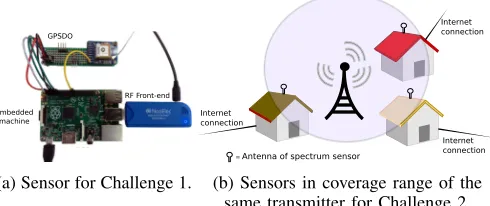
(a) Sensor for Challenge 1.

Internet connection Internet

connection

= Antenna of spectrum sensor

Internet connection

(b) Sensors in coverage range of the same transmitter for Challenge 2.

Fig. 1: Low-cost spectrum sensing nodes and spectrum simi-larity for crowdsourcing spectrum data decoding.

counterpart, limiting the effectiveness of a spectrum monitor-ing system. At the extreme end, we envision to use commodity hardware such as USB dongles for radio signal acquisition that cost not more than $12 using software available as open-source [16, 17]. The spectrum sensor used in this work is shown in Fig. 1a.

Challenge 2: The network bandwidth problem. The second

challenge is that the system requires the participation of users that may deploy the sensors at a location (such as their homes) with a limited network bandwidth. This bandwidth is not a concern for most crowdsourcing initiatives which collect averages of the power spectrum. Instead the collection of raw I/Q samples is necessary to decode the original information in the backend. This imposes a large volume of data which is several orders of magnitude higher than the power spectrum as collected in typical sensing contexts. The core idea we investigate in this work to address Challenge 2 is to exploit the similarity of the spectrum in the time domain in order to identify sensors that are in the coverage range of the same transmitters (as shown in Fig. 1b). The principle is to instruct from the backend the nodes to listen to the same frequency band of interest in separate time slots, thus alleviating the amount of I/Q samples to be sent from each node (and user). However, there is a fundamental problem in this approach that brings to the challenge discussed next.

Challenge 3: The need for a fine time synchronization. It

independent sensor entities, each responsible to monitor the spectrum in a given area and with fully autonomous decisions for signal detection and radio occupancy such as in the focus of related works [19, 21, 20, 11, 22]. The approach we propose requires a time synchronization in the order of the sampling rate of the signal to be decoded and up to the frequency bandwidth of the RF frontend(corresponding to sub-microseconds synchronization for our RF frontends).

Our contributions. We present and implement a system architecture able to collect the digitalized radio samples (out-put of the Analog-Digital Converter (ADC) of each sensor) of different sensors and to reconstruct and decode the signals in the backend. The collaborative approach alleviates the network bandwidth load used by each sensor by exploiting the similarity of the spectrum of nodes in the same coverage area. We provide the following key contributions:

• We introduce a distributed architecture for radio signal

monitoring and decoding using the digital samples col-lected by low-cost spectrum sensors (Section II).

• We propose different techniques to solve the problem of

timing synchronization among the sensors (Section III).

• We present a distributed time multiplexing mechanism

and introduce a Kalman filter model that operates in the backend. It is used to estimate and correct the relative time offset between pairs of sensors with a limited amount of uplink bandwidth usage (Section IV).

• We evaluate the system with a proof-of-concept using

real data from Long-Term Evolution (LTE) base stations (Section V).

• We make the sensing spectrum software available as open

source1_.

II. ARCHITECTURE FORCOLLABORATIVERADIOSIGNAL MONITORING ANDDECODING

This work considers the overarching goal of collecting digitalized radio samples of encoded signals transmitted over the air and decoding them in the backend. Next, we present the proposed architecture.

A. System components

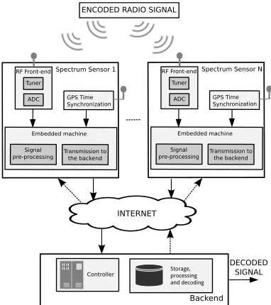
A high-level overview of the distributed system architecture for crowdsourcing radio signal monitoring and decoding is presented in Fig. 2. We can distinguish two main components, the sensors and the backend.

Spectrum sensors. We consider sensors such as the ones shown in Fig. 1a. We rely on a low-cost software defined-radio USB dongle for signal acquisition and a commodity embedded machine for signal pre-processing and transmission to the backend. Our hardware components are commercial off-the-shelf and among the cheapest currently on the market (total sensor cost of less than 100 $).

Ourradio signal acquisition hardwareis a RTL-SDR based

software-defined radio that acts as RF frontend, providing raw I/Q samples to the embedded machine over USB. The

1_{http://github.com/electrosense/sensing/}

Backend

Controller

INTERNET

Embedded machine

Signal

pre-processing Transmission tothe backend RF Front-end

Tuner

ADC GPS Time Synchronization

Spectrum Sensor 1

Embedded machine

Signal

pre-processing Transmission tothe backend RF Front-end

Tuner

ADC GPS Time Synchronization

Spectrum Sensor N

DECODED SIGNAL ENCODED RADIO SIGNAL

Storage, processing andedecoding

Fig. 2: High-level overview of the distributed system architec-ture for collaborative radio signal monitoring and decoding.

USB dongle can sample any radio frequency between 24 and 1766 MHz and send it to the embedded machine at a maximum rate of 2.4 MS/s without any sample losses.

The embedded machine is a RaspBerryPi (RPi), model

B+ with a CPU clocked at 700 MHz and 512 MB of RAM. A dedicated RPi software module accesses the RF frontend through the RTL-SDR library (librtlsdr from the OsmocomSDR project2_{) to retrieve raw I/Q samples in a}

con-figurable frequency band. The RPi then processes, compresses (loss-less compression making use of the zlib data compres-sion library [17]) and sends the samples to the backend through Internet using the on-board Ethernet interface.

Backend. The backend is a server or set of servers with sufficient large storage and computation capabilities. It con-tains the two main blocks shown in Figure 2. The controller block sends commands to the spectrum sensors and instructs them about the configuration scheme for data collection. The storage, processing and decoding block provides sufficient storage to save all I/Q samples and collaboratively recombines and decodes spectrum data.

B. Spectrum similarity for the network bandwidth problem

Transmitting raw I/Q samples to the backend requires a large volume of data. In order to alleviate this problem, we consider thatlow-cost sensors can allow a pervasive deploy-ment, with nodes belonging to users in the same neighborhood and observing a similar spectrum in the frequencies of interest.

Example. We consider two sensors with similarity in the

spectrum. The controller in the backend (c.f. Fig. 2) assigns time slots to each sensor to collect I/Q samples alternating the sensors in subsequent time slots (sensor 1in time slot 1,

sensor 2in time slot 2,sensor 1in time slot 3, etc.). Samples

0 0. 2 0. 4 0. 6 0. 8

Time offset (μs)

ECDF

GPSDO+RPi GPSDO+RPi+RF

0 100 200 300 400

Time (ms)

O

ff

se

t (

μ

s)

Continuous Sampling Start/Stop Sampling

100 ₁₀1 ₁₀2 ₁₀3 ₁₀4

1

0 0.025 0.05 0.075 0.1 0.125 0.15

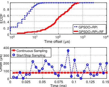
Fig. 3: GPSDO+RPi: time offset between spectrum sensors computed at the system level; GPSDO+RPi+RF: time offset for the acquisition of samples via the radio frontend (top). Comparison of the time offset, using continuous sampling strategy in both sensors and the start/stop sampling strategy in both sensors (bottom).

are sent bysensor 1andsensor 2to the backend. After signal processing and storing, the original signal is recombined and decoded. Considering slots of equal duration, this mechanism

alleviates the network bandwidth load of each user by a factor equal to the number of sensors in range of the same transmitter.

Recombining the original signal with partial data from multiple sensors requires a tight time synchronization among sensors. Otherwise, the decoder will not be able to correctly decode the signals transmitted over the air. However, precisely collecting I/Q samples in each sensor during the time slots assigned to is a difficult task given our software-defined and low-cost distributed sensor network architecture. In the next section, we study this problem in details.

III. TIMINGSYNCHRONIZATIONANALYSIS

In order to apply the time division approach presented in Section II-B, the backend requires a precision close to the sampling rate of the signal to be decoded in order to align the I/Q samples. This precision can be up to the frequency bandwidth of the RF frontend, which corresponds to

sub-microseconds time synchronization for our RF frontends. In

this section, we study the techniques we apply and the prob-lems we have to solve to guarantee this high precision of the time synchronization.

A. Precision with GPS disciplined oscillator

We embed a low-cost GPS disciplined oscillator (GPSDO) to improve the precision of the timing synchronization between pairs of spectrum sensors (see Fig. 1a). The GPSDO works as a stable time reference with nanosecond accuracy, and it is directly connected to the RPi as a global time reference using a General Purpose Input/Output (GPIO) pin. Using this pin, the GPSDO sends a Pulse Per Second (PPS) signal every second. In this way, the RPi knows when a second starts and

can correct any possible local clock drift. Local timestamps are then appended by the RPi to each single I/Q sample using the time reference provided by the GPSDO module.

Evaluation. We integrate the GPSDO module in two sen-sors and evaluate their relative time offset in two scenarios. In the GPSDO+RPi scenario, the two sensors are scheduled to execute a command (local timestamp acquisition) at a given absolute time. The offset is computed as the differ-ence of the local timestamps acquired in each sensor. In the

GPSDO+RPi+RFscenario, the sensors are scheduled to start

the RF sensing command to tune to the same central frequency at the same absolute time. The offset is computed by detecting the time shift between the signals captured by the two sensors (the methodology to detect the time shift is introduced in Section III-C). The results are plotted in Fig. 3 (top). We observe that the GPSDO does not suffice to achieve high precision (1µs or less) between sensors in both scenarios.

Results analysis. There are two fundamental reasons im-posed by our low-cost sensor hardware for the results in Fig. 3 (top). First, the minimum resolution of the embedded

machine software clock (i.e. of the RPi) is 1µs. Even with

the GPSDO as a time reference signal, Fig. 3 (top) shows that the 80th-percentile of the time offset between two sensors (GPSDO+RPi) remains up to 8µs. It follows that thissoftware clock is subjected to significant noise.

Second, the software-based signal acquisition transmits I/Q samples over the USB interface of the spectrum sensor. This

USB interface introduces significant jitter which manifests

itself in large sampling offsets between signals that are ac-quired by different sensors. Figure 3 (top) shows that the 80th-percentile time offset of two signals acquired by different sensors (GPSDO+RPi+RF) is about 278µs. Considering a sampling rate of 2.4 MS/s, an offset of 278µs results already in a signal misalignment of more than 600 samples.

B. Continuous sampling methodology

The results in the previous section demonstrate a significant relative time shift of the I/Q samples collected by independent spectrum sensors. We now instruct the two sensors to start and stop sampling at the same time and we compute the offset by detecting the time shift of the signals acquired. Fig. 3 (bottom) shows that the time offset between sensors varies over time with ranges between 0 and 400µs (0-800 I/Q samples). Such a large variation of the offset is undesired for the time division approach presented in Section II-B.

Time (seconds)

O

ff

se

t (

μ

s)

Cross-Correlation Beacon signal (PSS)

Time (seconds)

O

ff

se

t (

μ

s)

Pair of sensors #1 Pair of sensors #2

0 50 100 150 200

0 50 100 150 200

-2000 -1000 0 1000 2000 -200 0 200

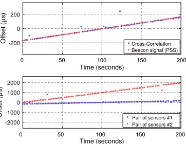
Fig. 4: Time offset computed using cross-correlation between signals and beacon signal detection (top). Each pair of RF frontend tuners has a different drift (bottom).

We observe a variation range of 8 I/Q samples over a short time, 100 times less than using the start/stop method.

There are two advantages of this methodology. First, it inherently reduces any delay caused by the main board for processing the requests to start and stop (embedded machine software clock). Second, it significantly reduces the drift caused by the communication between the main embedded board and the USB interface of the RF frontend. The approach of continuously sampling the radio can be applied also to the RPi B+ used in this work (an entry-level model), which features only one CPU core. In fact, the CPU speed is sufficiently faster than the sampling process, and it is capable of executing other tasks such as compressing and transmitting I/Q samples to the backend.

C. Technology independent offset computation

A longer trace over time of the continuous sampling ap-proach is shown in Fig. 4(top) where we can observe how the offset increases over the time. This implies that the internal clock of one of the RF frontend tuners works faster than the other one. In order to compute the relative offset, we have used a beacon signal detection mechanism (PSS signal of LTE, see also Section V-A). However, this method has the drawback of beingtechnology dependent. In fact, a beaconing signal is not always available, which calls for an approach which istechnology independent. We then propose to compute the relative offset between sensors using the cross-correlation between the I/Q samples collected by each sensor. Letxandy

be the complex vector of I/Q samples of two different sensors andrx,y[m]denote the cross-correlation of both vectors with a lag m. At time k, we then compute the time offsetµk as the maximum cross-correlation:

µk= arg max

m∈{−I,...,I}

rx,y[m] (1)

where I is the maximum lag. As shown in Fig. 4(top), we obtain similar offset values using both techniques. It follows

that we can rely on the maximum cross-correlation metric to

compute the time offset between spectrum sensors.

Sampling Sensor 1 Sampling Sensor 2

Chunk

Samples S1+S2

Sensor 1

Sensor 2

Backend

Time

Overlap Interval (I)

Fig. 5: Time multiplexing mechanism. The whole frequency band is covered by collecting I/Q samples from multiple sen-sors. Cross-correlation analysis is enabled by overlap intervals.

Figure 4 (bottom) shows that each pair of RF receiver has a different, but stable, drift over time. From Fig. 4 (bottom), we can infer that the offset largely depends on the pairs of sensors. Not shown in Figure, when changing the RPi boards and using the same pair of RF receivers, we observe a similar drift. This confirms that the offset depends on the pair of RF receivers, but not on the main embedded boards. For “pair of sensors 2”, the measured offset results in a relative drift equal to ≈73kHz. This is consistent with the reported high frequency instability (up to 50 ppm) of the low-cost onboard crystal oscillator of each RTL-SDR USB dongle [10].

IV. DISTRIBUTED TIME MULTIPLEXING

As explained in Section II-B, we want to assign different time slots to different sensors for I/Q sample collection. We have also seen that low-cost sensors impose significant limitations that affect the time synchronization among sensing nodes and that the correlation analysis provides a robust methodology to estimate the offset with continuous sampling (cf. Section III). However, three problems emerge:

• Assigning continuous and independent slots to different

sensors means that there is no spectrum data that can be used for correlation analysis.

• Even if we would be able to correctly estimate the time

offset between sensors, correcting this offset in the sensor would imply to stop the sampling process. In turn, this would affect the quality of gathered I/Q samples, as shown in Fig. 3 (top).

In order to solve these problems, we present in what follows our distributed time multiplexing mechanism to collect I/Q samples from different spectrum sensors for data decoding.

A. Overlap interval

We define time slots, calledchunks, that include anoverlap intervalI, in which I/Q samples are sent from more than one sensor to the backend. Figure 5 shows a schematic of the distributed sampling technique.Our idea is to use the overlap

interval I to perform correlation analysis as in Eq. (1) and

(a) It should be sufficiently large to ensure that the peak of the cross-correlation (time offset) can be found.

(b) It should be sufficiently small to not waste the uplink network bandwidth usage.

B. Estimation of the offset between pairs of sensors

We derive a model to estimate the offset and provide the correct alignment among sensors. Our model is based on a Kalman Filter (KF) that allows us to estimate the offset and drift more precisely that the one based on a single noisy measurement. The model supports the empirical observation that the offset increases as a linear function over time due to the drift between RF frontend tuners (cf. Section III).

The state vector that we want to estimate using the KF is

x=

O DT

whereO represents the offset andDthe drift, following this state model:

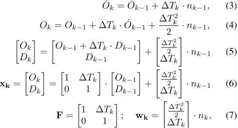
xk=F·xk−1+wk−1, (2)

To deriveFandwk, letOk andDk= ˙Okdenote respectively

the offset and the drift at time k. The second-order model is described by Ok¨ =nk where nk ∼ N(0, σ2

n) is an AWGN

(Additive White Gaussian Noise). We assume that the drift is constant for this model since the offset shown in Fig. 4 is linear over a sufficient large time period3_{. Thus, the choice of}

a very low value ofσn= 10−2_{. We derive the parameters of}

the state model as follow:

˙

Ok = ˙Ok−1+ ∆Tk·nk−1, (3)

Ok=Ok−1+ ∆Tk·Ok˙ −1+

∆Tk2

2 ·nk−1, (4) Ok Dk =

Ok−1+ ∆Tk·Dk−1

Dk−1

+

"

∆T2 k 2

∆Tk

#

·nk−1 (5)

xk=

Ok Dk = 1 ∆Tk

0 1

·

Ok−1

Dk−1

+

"

∆Tk2 2

∆Tk

#

·nk−1 (6)

F=

1 ∆Tk

0 1

; wk=

"

∆T2 k 2

∆Tk

#

·nk, (7) where ∆Tk =tk−tk−1 andtk represents the absolute time

at iteration k. For the KF measurement model, we have:

zk=G·xk+vk, (8) zk=

µk ∆µk = Ok

∆Tk·Dk

+vk (9)

zk= µk ∆µk = 1 0

0 ∆Tk

· Ok Dk

+vk (10)

G=

1 0

0 ∆Tk

(11)

whereµk is the output (lag) of the maximum cross-correlation analysis in presence of continuous sampling (cf. Eq. (1)).

wk ∼ N(0,Qk) and vk ∼ N(0,Rk) represent

respec-tively the process noise and the measurement noise that follow

3_{Effects such as the temperature can vary the offset, however they tend to}

occur at larger time scales than what we consider here, and can then be easily tracked with a small value ofσn.

[Input] Offset computed

among signals

Prediction measurement evaluation

Correction Offset estimated

[Input] Previous KF state estimated

Discarded Accepted

(Prediction + Correction)

Offset estimated

(Prediction)

Fig. 6: The Kalman filter correction step is applied only if the measurement µk is not discarded (it is not an outlier). Otherwise the time offset estimated for the next iteration will be computed using exclusively the prediction step.

Gaussian distributions with autocovariance matrices Qk and Rk. According to Eq. (7), we derive the following formulation

of Qk:

Qk=_E[wkwkT] = "_∆T4

k 4

∆Tk3 2 ∆T3

k

2 ∆Tk2

#

·σn2 (12)

For the autocovariance matrixRkof the measurement noise,

we use an adaptive estimation based on the covariance match-ing method originally introduced in the context of GPS posi-tioning. This method calculates the residualsˆ_νk =zk−G·ˆxk

that are the differences between the observation vectors zk

and their corresponding estimated values G·xk consistent with their theoretical values (ˆxk is the corrected state vector). Then, it calculates Rk based on these residuals computed in the lastw iterations [7].

As the KF assumes that the measurement noise is Gaussian distributed, any measurement outlier can negatively affect the filter. We propose a method to determine if the current measurement µk can be used to correct the prediction of the KF and improve the estimation. Figure 6 shows that the new offset estimation is based on the prediction+correction

steps only if the new measurement is accepted. Otherwise, only the prediction step is used to estimate the offset. The current measurement is accepted if it is not an outlier. This evaluation method is based on the median calculation using the last estimates. Measurement values higher than a certain threshold are considered asoutliersand discarded.

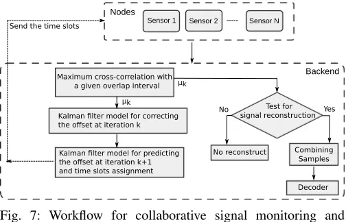
C. Signal reconstruction and decoding

Figure 7 shows the workflow to reconstruct the signal and decode it using I/Q samples received from a set of sensors. The first step is to align the signals in time using the overlap intervalI. In case of two sensors, the overlap interval contains samples from both sensors. Using the raw I/Q samples of this overlap interval, we compute thecross-correlationfor different lags to determine the time offsetµk between pairs of sensors. This offset is used in the data decoding step for iteration k

and time slots assignment for iterationk+ 1.

Sensor 1 Sensor N Nodes

Maximum cross-correlation with a given overlap interval

Combining Samples

Decoder eest for signal reconstruction Yes No

No reconstruct

Sensor 2

Send the time slots

Backend

Kalman filter model for predicting the offset at iteration k+1 and time slots assignment

μk

μk

Kalman filter model for correcting the offset at iteration k

Fig. 7: Workflow for collaborative signal monitoring and decoding.

• Low spectrum similarity. If µk is lower than a given

threshold, spectrum sensors are too far apart (they are not listening to the same transmitter), or the overlap interval

Ik is too small to mitigate the misalignment of the signals.

• High spectrum similarity. If µk is equal or above the

threshold, we can proceed with signal combining and decoding.

In the latter case, we align the sequences of I/Q samples from pairs of sensors using the valueµk. While this technique can be performed independently at each iteration, it is affected by noisy samples and the cross-correlation computation may erroneously declare the lag with the highest correlation value. In order to increase the robustness of the offset estimation, we also consider an estimator that uses the last N iterations of overlap intervals {Ik−N−1, Ik−N−2, . . . , Ik},and gives as

output the sequence of drift estimations. Since the drift is approximately constant over a sufficiently short period (cf. Fig. 4), using the last N subsequent overlap intervals, the

aligned+median technique takes as output the median of the

sequence of drift estimations and converts it to the offset between pairs of sensors. Finally, the backend aligns the sequences of I/Q samples received from different sensors and it combines them in one sequence for data decoding. The decoder is unaware that the sequence of I/Q samples has been received with inputs from multiple sensors, and decodes the signal using standard demodulation and decoding techniques. Time slots assignment for iteration k+ 1.Each spectrum sensor continuously collects I/Q samples, and the controller compensates their relative offset by anticipating or delaying the sequences of retrieved I/Q samples from each sensor accordingly. We start with µk as input (measurement model) of the KF model introduced in Section IV-B. The output of the KF gives the corrected time offset and drift xkˆ between pairs of spectrum sensors. As studied in Section IV-B, the KF correction step is applied only ifµkis not an outlier. Otherwise this step is bypassed. Finally, the KF model predicts the offset for the iteration k+ 1 using the prediction step of the KF model, and uses it to assign the time slots in each sensor to compensate for their relative offset.

V. EVALUATION

We evaluate our approach using LTE signals in the 801-811 MHz frequency band. Our analysis combines both simulation and real scenarios. The simulation scenario focuses on the impact of the offset among signals and how the noise affects the signal reconstruction. On the other hand, the practical analysis focuses on the evaluation of the different sampling strategies and the effect in the performance when the offset is estimated and corrected.

A. LTE

We first briefly review the main LTE concepts that are necessary for the evaluation. LTE defines two structures:frame

andsubframe. Aframe is a structure represented in the time domain with a duration of 10 ms. Each frame contains 10

subframes of 1 ms duration and each subframe contains 7

OFDM symbols. An OFDM symbol corresponds to a variable number of samples depending on the system bandwidth. The

UE (User Equipment) needs to get a cell id, a time slot

and a frame synchronization in order to perform any more complex operation in a given network. The first step for the UE is to scan different frequencies and search for the PSS (Primary Synchronization Signal) and SSS (Secondary Synchronization Signal), which have a band of1.4MHz. The PSS and SSS are located in subframes 0 and 5 of every frame. Since each subframe is 1ms long, this means the UE can synchronize every 5ms. Once the PSS is detected, the SSS is always located one OFDM symbol earlier. The PSS is a frequency-domain Zadoff-Chu [6] sequence and provides the

layer identity(0 to 2). The SSS codes thecell identityas 1 out of 168 pseudo random sequences which are BPSK modulated. Decoding the PSS and SSS properly, we obtain the Physical Cell ID(PCI) as:PCI = 3×(cell identity) + layer identity. To decode the PCI, the minimum sampling rate is1.92MS/s, which implies that an OFDM symbol is 128 I/Q samples long. We use the LTE-Cell-Scanner4_{to decode the LTE channel cell}

id.

B. Emulation with real data

In this experiment, spectrum data is collected from one sin-gle sensor that scans continuously with a center frequency of 806 MHz. With this data, our simulation environment creates two datasets using the following configuration:chunk size = 100I/Q samples andoverlap interval = 20I/Q samples. We introduce artificial time offsets and add Gaussian noise to one copy of the signal in order to understand the impact of sensor synchronization errors and noise on the signal recombining and decoding process. We set the threshold correlation value to determine if there is sufficient similarity or not for signal reconstruction equal to0.65(cf. Section IV-C). We recombine the signal in time using these two datasets and finally decode the control information of the LTE channel.

Figure 8a shows the cross-correlation value and decoding success rate for different techniques and different offsets. The

0 2 4 6 8 10 12 14 16 0

0.2 0.4 0.6 0.8 1

Offset (I/Q samples)

Correlation

0 2 4 6 8 10 12 14 16

0 20 40 60 80 100

Offset (I/Q samples)

DSR (%)

not aligned aligned aligned+median

(a) No noise.

0 2 4 6 8 10 12 14 16

0 0.2 0.4 0.6 0.8 1

Offset (I/Q samples)

Correlation

not aligned aligned aligned+median

0 2 4 6 8 10 12 14 16

0 20 40 60 80 100

Offset (I/Q samples)

DSR (%)

(b)SNR = 10_dB

Fig. 8: Average correlation (top) and decoding success rate (DSR) applying different artificial offsets and several tech-niques to reconstruct the signal (bottom) (chunk size = 100I/Q andoverlap interval = 20I/Q).

10 15 20 25 30 35 40

0 20 40 60 80 100

SNR (dB)

Decoding Success Rate (%)

not aligned aligned aligned+median

Fig. 9: Decoding success rate applying different SNR values and evaluating the signal reconstruction techniques (offset = 10I/Q,chunk size = 100I/Q,overlap interval = 20I/Q).

aligned technique can decode the signals in the simulation

environment with a high success rate as long as the offset is not higher than 40% of the overlap interval. In addition,

the aligned+mediantechnique can decode the signals as long

as the offset is not higher than 50% of the overlap interval. These results outperform thenot-alignedtechnique that simply assumes there is no time offset between signals and computes the cross-correlation without shifting on the overlap area of both datasets (therefore, it only works with an offset equal to 0).

We also evaluate the impact of the noise. In order to conduct this experiment, we add AWGN noise to one of the signals. The results are shown in Fig. 8b. For the evaluation, we set the signal-to-noise ratio equal to SNR = 10dB. Thealignedand

aligned+mediantechniques reduce their success rate, but it is still possible to decode the signal when the offset is lower than 20%and30%of theoverlap interval, respectively. We finally evaluate the robustness of the different techniques in presence of various levels of noise and offset = 10I/Q. Figure 9 shows that the aligned-mediantechnique clearly outperforms the other two methods.

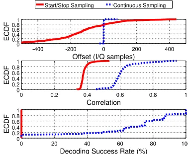
C. Real scenario

In this experiment, two sensors are located three meters from each other, scanning in the center frequency of806MHz (wavelength is 0.37 meters) with a sampling rate of1.92MS/s

-400 -200 0 200 400

0 0.2 0.4 0.6

0.81

Offset (I/Q samples)

ECDF

Start/Stop Sampling Continuous Sampling

0 20 40 60 80 100

0 0.2 0.4 0.6 0.8 1

Decoding Success Rate (%)

ECDF

0 0.2 0.4 0.6 0.8 1

0 0.2 0.4 0.6 0.8 1

Correlation

ECDF

Fig. 10: Evaluation of the offset (top), correlation (middle) and decoding success rate (bottom) between the start/stop and continuous scanning strategies using real spectrum data coming from two different sensors (chunk size = 100I/Q, overlap interval = 20I/Q).

(complex samples). In our envisioned crowdsourcing scenario, sensing nodes may be located farther apart but this reference scenario serves as a baseline to understand the decoding performance when sensors receive almost identical signals. As in the previous section, we compare the decoding success rate using different sampling techniques. In these experiments, we compare the sampling process using the start/stop approach and the continuous approach introduced in Section III-B. This experiment is executed 300 times. Each time, the generated dataset contains between 15 and 18 PSS-SSS signals, corre-sponding to a total of more than 4000 SSS-PSS.

As explained in Section III-B, the start/stop sampling ap-proach introduces a large and unpredictable offset. This im-plies that the overlap areas are misaligned and the correlation value is low. Figure 10 (top) shows how the offset spans a very large set of values, and therefore the correlation value is not enough to obtain reliable decoding information. However, the continuous sampling approach allows to keep the overlap interval aligned thanks to the KF model proposed in this work. As shown in Fig. 10 (middle), the correlation value increases when applying the continuous sampling technique since the overlap intervals are aligned. We finally evaluate the impact on the decoding success rate in Fig. 10 (bottom). While the correlation for start/stop sampling does not guarantee reliable decoding (with values close to zero), the decoding success rate is highly improved with the proposed continuous sampling approach, making the system functional.

D. Evaluation of the Kalman filter model for offset estimation

We study the accuracy of the KF model using the same setup scenario of Section V-C and we present the results in Fig. 11. First we consider the case of a long overlap interval (10,000 samples) which guarantees that the maximum of the offset can be easily found with the technology independent

0 50 100 150 200 250 300 350 -300

-200 -100 0 100

Time (ms)

O

ff

se

t (

s)

estimated offset (10000 I/Q) estimated offset (5000 I/Q) estimated offset (500 I/Q) real offset (10000 I/Q)

0 50 100 150 200 250 300 350

-150 -100 -50 0 50

Time (ms)

O

ff

se

t err

or (

s)

estimation error (10000 I/Q) estimation error (5000 I/Q) estimation error (500 I/Q)

μ

μ

Fig. 11: Estimated offset (top) and estimation error (bottom) using the proposed Kalman Filter model.

I/Q samples (“estimated offset (10000)”) shows that the filter has the same performance as the real offset (computed using

the technology dependentapproach in Section III-C).

As explained in Section IV-A, a smaller overlap interval should be preferred to reduce the load of the uplink bandwidth of users. We then evaluate the accuracy of the filter with smaller overlap intervals. As expected, the convergence is slightly slower. Yet, as shown in Fig. 11 for 500 and 5,000 I/Q samples, the filter is always able to converge to the true offset. The KF model adapts well to different conditions. For instance (not shown in figure), it estimates an average standard deviation of the offset for 500 I/Q samples that is more than 15 times larger than for 10,000 I/Q samples. This shows that the estimated autocovariance matrixRkof the measurement noise

can deal with more noisy data observed with a smaller overlap interval I, and it automatically assigns a standard deviation that tends to increase when the overlap interval I decreases.

We then study the decoding success rate for different chunk sizes and using a small overlap interval (20 I/Q). The baseline is represented by one sensor scanning in its assigned time slots. We present the results in Fig. 12. In the case that the KF model is not applied, the decoding success rate decreases considerably for almost all chunk size values. Here, the overlap intervals are misaligned and the predicted offset is not corrected. For all the different chunk sizes, the collaborative sampling approach using the KF model provides a high decoding success rate of the signals recombined from the I/Q samples of two sensors.

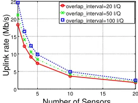
E. Uplink network bandwidth

One of the important benefits to use the collaborative approach for signal reconstruction and decoding is that it can reduce the uplink bandwidth used by each single sensor. One single node scanning continuously a LTE channel at1.92MS/s would need an uplink bandwidth of about 36.8Mb/s to send all I/Q samples to the backend using a compression factor of 70%. Depending on the number of sensors and the sampling configuration parameters of the system (chunk size and overlap interval), the uplink network bandwidth for each sensor can

102 ₁₀3 ₁₀4

0 20 40 60 80 100

Chunk Size (I/Q samples)

Decoding Success Rate (%)

Baseline (1 sensor) Collaborative sampling (KF) Collaborative sampling (non-KF)

Fig. 12: Decoding success rate of cell id (overlap interval = 20I/Q).

5 10 15 20

0 5 10 15 20 25

Number of Sensors

Uplink rate (Mb/s)

overlap_interval=20 I/Q overlap_interval=50 I/Q overlap_interval=100 I/Q

Fig. 13: Uplink bandwidth used by each sensor.

be reduced. Figure 13 shows in simulations how the uplink network bandwidth decreases considering a set of sensors in range of the same transmitter. The crowdsourcing approach clearly allows to relieve the network bandwidth per user.

VI. RELATED WORK

Large corporations have shown interest in the topic of large-scale spectrum sensing. Google has lunched the Spectrum Database [4], a joint initiative between Google, industry and regulators to make more spectrum available by using a database to enable dynamic spectrum sharing in TV white spaces. They provide an access to the data to query white space availability based on time and location. Microsoft Spectrum Observatory [5] is a platform with a high cost (approximately 5000 dollars per node). Using data collected with the Spectrum Observatory, [22] proposed a system that identifies transmitters from raw spectrum measurements without prior knowledge of transmitter signatures. SpecNet [11] is a platform developed by Microsoft Research that the scientific community can use to remotely schedule spectrum measurements in real-time in order to study the spectrum usage. Electrosense [2] and BlueHorizon [1] are crowdsourced architectures that allow to share spectrum information. In contrast to the works above, the sensors in our system work collaboratively with the over-arching goal of reconstructing and decoding a radio signal transmitted in the backend.

threshold. [13] introduced the idea of cooperative sensing where a certain frequency spectrum is monitored distributively with different sensing nodes. [9] proposed to use a cooperative environment to distinguish between an unused band and deep fade due to shadowing or fading effects. That work has been studied only by means of simulations. [8, 18] employed correlation techniques in different environments, but the study is based on simulations only. No system architecture problems were studied in these works for their actual implementation. In addition, unlike classical collaborative decoding [15] and cooperative diversity schemes [12], the sensors in our work are not performing the physical-layer decoding, but just provide interleaved measurements of raw I/Q samples which are stored and decoded in the backend. SpecInsight was introduced in [19] and is a system for acquiring 4 GHz of spectrum in real-time using USRP radios with tens of MHz in 7 locations in the US. Because of the high-end platform used in their work, there are little opportunities for pervasive deployments. [17] proposed different frequency hopping strategies to overcome the hardware limitations of low-cost radios. These systems considered spectrum data in the frequency domain, while we consider data in the time domain (I/Q samples), posing new challenges, as discussed in this paper.

VII. CONCLUSION

We have studied the problem of crowdsourcing spectrum data decoding using low-cost software defined radios. We have addressed the main challenges and proposed a distributed approach and several techniques and strategies for sampling the spectrum collaboratively. Our approach can reconstruct the signal based on raw I/Q samples received by different low-cost sensors, all in range of the same transmitter, solving problems such as the sub-microsecond level time synchronization re-quired between independent sensors deployed by the users. We have provided an evaluation with real LTE signals and shown the feasibility to reconstruct and decode signals in a crowdsourcing scenario with low-cost sensors.

ACKNOWLEDGMENTS

This work has been funded in part by the European Commission in the framework of the H2020-ICT-2014-2 project Flex5Gware (Grant agreement no. 671563), in part by the grant TEC2014-55713-R Hyperadapt and by the Madrid Regional Government through the TIGRE5-CM pro-gram (S2013/ICE- 2919). We thank the anonymous reviewers for their valuable comments and suggestions.

REFERENCES

[1] Blue horizon ibm. http://bluehorizon.network/documentation/ poc3-radio-spectrum-analysis.

[2] Electrosense. https://electrosense.org/. [3] Gnu radio. http://gnuradio.org/.

[4] Google spectrum database. http://www.google.com/get/ spectrumdatabase/.

[5] Microsoft spectrum observatory. http://observatory. microsoftspectrum.com/.

[6] E. U. T. R. Access. Physical channels and modulation. 3GPP TS, 36.211:V8, 2016.

[7] A. Almagbile, J. Wang, and W. Ding. Evaluating the perfor-mances of adaptive Kalman filter methods in GPS/INS integra-tion. Journal of Global Positioning Systems, 2010.

[8] A. S. Cacciapuoti, I. F. Akyildiz, and L. Paura. Correlation-aware user selection for cooperative spectrum sensing in cog-nitive radio ad hoc networks. IEEE JSAC, 2012.

[9] A. Ghasemi and E. S. Sousa. Collaborative spectrum sensing for opportunistic access in fading environments.IEEE DySPAN 2005.

[10] M. Higginson-Rollins and A. E. Rogers. Development of a low cost spectrometer for small radio telescope (srt), very small radio telescope (vsrt), and ozone spectrometer. 2013.

[11] A. Iyer, K. K. Chintalapudi, V. Navda, R. Ramjee, V. Padmanab-han, and C. Murthy. Specnet: Spectrum sensing sans fronti`eres. USENIX, 2011.

[12] J. N. Laneman, D. N. C. Tse, and G. W. Wornell. Cooperative Diversity in Wireless Networks: Efficient Protocols and Outage Behavior.IEEE Transactions on Information Theory, 50, 2004. [13] S. Mishra, A. Sahai, and R. Brodersen. Cooperative Sensing among Cognitive Radios. 2006 IEEE International Conference on Communications, pages 1658–1663, 2006.

[14] J. Naganawa, H. Kim, S. Saruwatari, H. Onaga, and H. Morikawa. Distributed spectrum sensing utilizing heteroge-neous wireless devices and measurement equipment. InIEEE DySPAN 2011.

[15] A. Nayagam, J. M. Shea, and T. F. Wong. Collaborative De-coding in Bandwidth-Constrained Environments. IEEE JSAC, 2007.

[16] A. Nika, Z. Li, Y. Zhu, Y. Zhu, B. Y. Zhao, X. Zhou, and H. Zheng. Empirical validation of commodity spectrum moni-toring. ACM SenSys ’16.

[17] D. Pfammatter, D. Giustiniano, and V. Lenders. A Software-defined Sensor Architecture for Large-scale Wideband Spectrum Monitoring. ACM/IEEE IPSN ’15.

[18] M. Sampietro, G. Accomoando, L. G. Fasoli, G. Ferrari, and E. C. Gatti. High Sensitivity Noise Measurement with a Correla-tion Spectrum Analyzer.IEEE Transactions on Instrumentation and Measurement, 49(4):1–3, 2000.

[19] L. Shi, P. Bahl, and D. Katabi. Beyond sensing: Multi-ghz realtime spectrum analytics. InNSDI ’15.

[20] M. Souryal, M. Ranganathan, J. Mink, , and N. E. Ouni. Real-time centralized spectrum monitoring: Feasibility, architecture, and latency. InIEEE DySPAN, 2015.

[21] T. Zhang, N. Leng, and S. Banerjee. A vehicle-based measure-ment framework for enhancing whitespace spectrum databases. ACM MobiCom ’14.