Applications of loudness models in audio engineering

(1)

The School of Computing and Digital Technology

Faculty of Computing, Engineering and the Built Environment

Birmingham City University

Applications of Loudness Models in Audio

Engineering

Dominic Ward

(2)

Abstract

This thesis investigates the application of perceptual models to areas of audio engineering, with a particular focus on music production. The goal was to establish efficient and practical tools for the measurement and control of the perceived loudness of musical sounds. Two types of loudness model were investigated: the single-band model and the multiband excitation pattern (EP) model. The heuristic single-band devices were designed to be simple but sufficiently effective for real-world application, whereas the multiband procedures were developed to give a reasonable account of a large body of psychoacoustic findings according to a functional model of the peripheral hearing system. The research addresses the extent to which current models of loudness generalise to musical instruments, and whether can they be successfully employed in music applications.

The domain-specific disparity between the two types of model was first tackled by reducing the computational load of state-of-the-art EP models to allow for fast but low-error auditory signal processing. Two elaborate hearing models were analysed and optimised using musical instruments and speech as test stimuli. It was shown that, after significantly reducing the complexity of both procedures, estimates of global loudness, such as peak loudness, as well as the intermediate auditory representations can be preserved with high accuracy. Based on the optimisations, two real-time applications were developed: a binaural loudness meter and an automatic multitrack mixer. This second system was designed to work independently of the loudness measurement procedure, and therefore supports both linear and nonlinear models. This allowed for a single mixing device to be assessed using different loudness metrics and this was demonstrated by evaluating three configurations through subjective assessment. Unexpectedly, when asked to rate both the overall quality of a mix and the degree to which instruments were equally loud, listeners preferred mixes generated using heuristic single-band models over those produced using a multiband procedure.

(3)

Acknowledgements

Firstly, I must acknowledge my supervisor Cham Athwal. He has guided me throughout this long journey and always made himself available when I needed support, even at difficult times. Cham’s continued encouragement, reassurance, motivation and belief in me was paramount to me completing this thesis.

I would like to express my gratitude to Joshua Reiss for his involvement in my work; his ideas and advice have been invaluable. Furthermore, a big thank you to Munevver K¨ok¨uer for her attention to detail and teaching me the ways of LA_TEX.

I’d like to acknowledge my colleagues at DMT Lab for fun times amidst interesting technical discussions: Ryan Stables, Matthew Cheshire, Yonghao Wang, Gregory Hough, Ian Williams, Sam Smith, Alan Dolhasz and Izzy MacLachlan. A special thanks to Sean Enderby for clarifying many technical issues and being a robust sounding board when battling concepts out with myself. I would also like to thank the Sound Engineering students at Birmingham City University, especially those who took the time to participate in my listening experiments.

Thanks to Esben Skovenborg for his patience and maintained interest, despite being attacked by my perpetual questions about regression models he fit 10 years ago. Similarly, thanks to Brecht De Man for many fruitful discussions about our research. Furthermore, I am grateful for the invaluable techniques and skills I have developed during my time at The University of Birmingham. Alan Wing, Mark Elliot, Winnie Chua and Caroline Palmer thanks for all your support. I would also like to acknowledge the following people for sharing code and clarifying implementation-level details: Harish Krishnamoorthi, Brian Moore and Brian Glasberg.

(4)

Introduction

Most normal-hearing people are well-versed in adjusting the level of their television or radio to achieve a comfortable listening experience. If the level of a subsequent commercial or song increases considerably, the listener will soon attenuate the reproduction to re-stabilise their sensory environ-ment. The ‘level-correction’ process is subjective—how loud is comfortable for me? Though this may be the case, there is a consensus among listeners when judging the perceived strength -the

loudness - of sound (Stevens 1955; Florentine 2011). Without this inter-listener consistency, our

daily interactions would be very awkward indeed!

This thesis investigates objective methods to predict the subjective loudness of sound, such that practical tasks, including volume adjustment, can be performed automatically to a standard that falls within the general agreement of a group of listeners. In particular, this project concentrates on the modelling of loudness of musical sounds commonly found in popular music, and developing tools to aid audio engineers with the many complex processes involved in music production.

The next section introduces perceptual models for loudness estimation and their application in audio engineering and music production. Following this overview, problems are highlighted to arrive at the thesis aim and objectives, an outline of the overall thesis is given, and the publications arising from the research are listed.

1.1

Loudness models

Hearing models can be divided into two types: perceptual (or psychoacoustic) models and phys-iological models. The former describe and predict the relationship between the stimulus and the percept, whereas the latter draw correlations between changes in the physical properties of the stimulus and the physiological responses they invoke (Florentine 2011). The two types of model are not mutually exclusive; although perceptual models are designed to account for psychophys-ical data, they too draw from knowledge gained from physiologpsychophys-ical measurements of the hearing organ, but to a far lesser degree than models of hearing anatomy and physiology. From a sci-entific perspective, the end goal of auditory modelling is to arrive at a general theory of hearing that encapsulates pertinent physiological and psychophysical knowledge (Meddis et al. 2010). Yet, sophisticated models of the auditory system are not necessary for many practical applications.

(9)

Chapter 1. Introduction

the level of detail of present perceptual loudness models. For example, the growth in loudness of the pure tone is adequately described by a simple power-law function of stimulus intensity. However, as more variables are added to the experimental recipe, such as the frequency of the tone, the psychological response becomes more complex, requiring a more refined model with multiple parameters. This bottom-up approach leads to procedures of considerable complexity as scientists continue to test hypotheses concerning the underlying mechanisms, uncovering a plethora of perceptual effects along the way. The most sophisticated of methods are those that characterise the three stages of auditory periphery: the outer, middle and inner ear. In short, the frequency dependency of loudness, as characterised by the equal-loudness contours, is primarily accounted for by the transmission of sound through the outer and middle ear. Then, a decomposition of the sound at the cochlea into different frequency bands—the critical bands of the hearing system—is necessary to predict the effect of spectral bandwidth on loudness. This latter phenomenon, known as spectral loudness summation (SLS), is theorised to be the result of the active filtering taking place inside the inner ear. Although primarily a predictor of loudness, the modelling of cochlear activity, or neural excitation, yields intermediate representations of sound, such asexcitation and specific loudness (SL) patterns. Therefore, in addition to predicting various loudness phenomena, these excitation pattern (EP) loudness models can also be used to calculate auditory masking effects. This peripheral-ear modelling approach also facilitates the simulation of impaired loudness perception in individuals with reduced cochlear sensitivity.

Another type of perceptual loudness model is the frequency-weighted energy measurement. These devices are essentially physical measures of sound intensity, but include a frequency-dependent attenuation to approximate the ear’s sensitivity at different frequencies. Once such device is the sound pressure level (SPL) meter, typically used for quantifying the loudness of environmental and industrial noise. Unlike the hearing system, these devices operate linearly with respect to sound level, and as such they offer different pre-emphasis filters, such as A and C weightings, which are to be manually activated by the user depending on the noise level. The A curve, for example, mimics the reduced sensitivity of the ear to low frequencies for softer sounds, whereas the C curve is comparatively broadband, designed for measuring the loudness at relatively high intensities. Because these devices do not include an elaborate filter bank, they are inherently simpler in design compared to the multiband approach, but consequently cannot predict complex psychoacoustic effects such as SLS.

1.1.1

Applications in audio engineering

(10)

Perhaps the most elementary yet prevalent application of a loudness model is loudness normal-isation or alignment, e.g. given sound A and sound B, make them equally loud. Such a scheme is often an important aspect of experiment design in order to counteract potential biasses introduced by differences in inter-stimulus loudness. It is rarely the case that physical signal metrics are accurate for loudness alignment (see Bech and Zacharov (2006)[Ch.8]). The practical importance of loudness normalisation is evident by the extensive work conducted by the Special Rapporteur Group (SRG) of the International Telecommunication Union Radiocommunication Sector (ITU-R), to address the problem of loudness fluctuations of programme material used in broadcasting, such as dialogue and music. This resulted in an internationally standardised objective loudness measure (ITU-R BS.1770 2006) which was found to work reliably well on a range of programme content (Soulodre et al. 2003; Soulodre and Norcross 2003; Skovenborg and Nielsen 2004b; Soulodre 2004; Soulodre and Lavoi 2005) and was later revised by the European Broadcast Union (EBU) for indus-try deployment (EBU R 128 2010; EBU Tech 3341 2011). The subsequent ITU-R BS.1770 (2015) single-band processor includes an adaptive gate to exclude quiet periods from the foreground, and can be applied to multichannel setups, e.g. surround sound, making it both robust and versatile. Despite its simplicity, the levelling paradigm has been embraced by the broadcasting and music production communities as a shield to defend against excessive dynamics compression and to realise consistent listening levels for the end listener (Camerer 2010).

One particular field of research where loudness models have received great interest is Intelligent Music Production (IMP), the goal of which is to develop intelligent systems to assist both amateur and professional audio engineers with music production. Here, the engineer mustlisten, manage and process multiple sound sources, called tracks, simultaneously, often in front of a live audience, such that the mixture is aesthetically pleasing to the listener. This technically demanding and creative task requires years of practical experience and domain-specific knowledge to execute to a high standard. Consequently, new forms of multichannel signal processors that analyse the re-lationships between the different tracks have been developed to assist humans with this complex time-consuming task (Reiss 2011). An example of this is the automatic fader controller, a device that sets the levels of a multitrack recording automatically by comparing inter-track sound fea-tures. Rather than use simplistic signal metrics, efficient single-band loudness models have been incorporated to better approximate the engineer’s hearing sensitivity to the different instruments comprising the mix (Gonzalez and Reiss 2009; Mansbridge et al. 2012b). The majority of IMP systems, especially those capable of real-time online processing, are based on single-band loudness models, such as the BS.1770 algorithm and EBU variants (EBU Tech 3341 2016).

(11)

representations (Hafezi and Reiss 2015).

1.2

Problems

There is a clear need for models of perceived loudness, yet with different modelling strategies and domains of application, it is not yet apparent which methods are best suited to music production. At first sight, the solution appears to incorporate algorithms that have been developed and vali-dated on broadcast material, especially considering their simplicity. But, broadcast content isnot the primary type of sound worked upon by music producers. Indeed, Pestana and Alvaro (2012) discovered inadequacies of the BS.1770 algorithm when applied to single instruments. Similarly, multiband models show high predictive power when simulating psychophysical experiments involv-ing stimuli synthesised in the laboratory, but music producers do not mix pure tones (fortunately). The current state-of-the-art in IMP assumes that the elaborate psychophysical models are better suited to complex musical sounds because they are grounded in auditory theory and can pre-dict masking effects. Yet, these perceptually-motivated mixing devices have not been subjectively evaluated or compared against alternative features.

One big advantage of employing a sophisticated perceptual model is the ability to quantify masking when combining different sounds (Aichinger et al. 2011). Frequency masking is a known hurdle for novices of music production, because it requires knowledge of the spectro-temporal in-teractions between all elements in the mix. Furthermore, frequency masking is hard to combat without accurate use of frequency equalisation, dynamics processing and good level/image balanc-ing. Senior (2011, p. 172) succinctly emphasises the complexities brought on by auditory masking when discussing the importance of equalisation: ‘The ramifications of frequency masking for mix-ing are enormous.’ In practice, the computational complexity of these multiband algorithms often restricts their application to real-world problems, especially in music production where multiple tracks play simultaneously.

To summarise, a promising yet underdeveloped area of research is the use of loudness models to quantify perceptual phenomena for use in audio engineering. In theory, procedures that include an inner-ear stage should better capture the experience of the listener because they have proved essential for describing a large body of psychophysical data. Unfortunately, the ability of such methods to generalise beyond the laboratory to the real-world, especially in music production, is relatively unknown. In addition, their high computational complexity makes them unattractive candidates for many practical applications (Krishnamoorthi 2011; Burdiel et al. 2012; Francombe et al. 2015; Wichern et al. 2015; De Man et al. 2017).

1.3

Thesis objectives

The aim of this thesis is to evaluate and extend current loudness modelling strategies for practical use in audio engineering, with a particular emphasis on music production. Not only does this research hope to contribute to improving the ear of the digital mixing assistant, but also advance scientific knowledge in loudness modelling. Accordingly, the primary objectives of this thesis are as follows:

1. To evaluate the performance of state-of-the-art loudness models when applied to musical sounds.

(12)

3. To establish new validated procedures for measuring the loudness of single instruments. 4. To develop a real-time mixing framework that accommodates both linear and nonlinear

loudness estimators to perform perceptually-motivated music mixing.

1.4

Thesis structure

Chapter 2 presents an overview of sound acoustics, the peripheral hearing system, and core prin-ciples of psychoacoustics. This review provides the necessary information to understand the basic mechanisms of the ear, and therefore the architecture of modern hearing models. Empirical psy-choacoustic findings are reported on to give insight into perceptual phenomena such as loudness and masking.

Chapter 3 provides a historical overview of loudness models before detailing computational methods, namely single-band and multiband procedures. Methods for analysing steady-state and time-varying sounds are discussed. In the latter case, a detailed analysis of their implementa-tion and funcimplementa-tionality is carried out—a necessary prerequisite for Chapter 4. The final secimplementa-tions compare the predictions of both standardised and recent multiband procedures to gain a deeper understanding of their practical differences when predicting the loudness of the type of sounds they were designed for. In addition, hypotheses relating the processing of the ear to the measured subjective psychological responses are investigated using different modelling techniques.

Chapter 4 presents an efficient realisation of a well-established multiband model for computing internal representations of dynamic sounds and measures of loudness. Prior work is presented, extended and evaluated using musical instruments and speech as test stimuli. Alternative low-complexity approaches to pre-cochlear filtering are given which are shown to outperform the original specification in terms of predicting absolute thresholds of pure tones. A parameterised implementation of the model is then presented and practical implications of different configura-tions are discussed. Finally, these techniques are used to realise fast adaptaconfigura-tions of two different loudness models in the form of a real-time binaural loudness meter. The meter is assessed through an objective analysis of the discrepancies in the auditory features introduced by the proposed techniques.

A real-time automatic fader controller for mixing multitrack audio is presented and evaluated in Chapter 5. The system is assessed through subjective listening tests, giving a preliminary insight into the predictive nature of the multiband model first adapted in Chapter 4 when applied to musical instruments. Additional considerations such as inter-track masking and relative loudness are discussed within the context of music mixing. The results of this preliminary evaluation motivate subsequent work in this thesis.

(13)

and those reported in prior work.

The body of work conducted in this thesis is summarised in Chapter 8 by highlighting key findings and discussing them in relation to the objectives introduced in Section 1.3. The thesis contributions are presented and directions for future work are suggested based on a critical analysis of the methods employed.

1.5

Publications

The following publications are associated with the work carried out in this thesis:

1. Ward, D., Reiss, J. D., and Athwal, C. (2012). “Multi-track mixing using a model of loudness and partial loudness”. In: Proceedings of the 133rd _{Audio Engineering Society Convention.}

2. Ward, D., Athwal, C., and Kokuer, M. (2013). “An efficient time-varying loudness model”.

In: Proceedings of the IEEE Workshop on Applications of Signal Processing to Audio and

Acoustics.

3. Ward, D., Enderby, S., Athwal, C., and Reiss, J. D. (2015). “Real-time excitation based binaural loudness meters”. In: Proceedings of the 18th _{International International Conference}

on Digital Audio Effects

4. Ward, D. and Reiss, J. D. (2016). “Loudness algorithms for automatic mixing”. In:

Pro-ceedings of the 2nd _{Audio Engineering Society Workshop on Intelligent Music Production}

(14)

The Hearing System

When conversing with a friend it is necessary to adapt to our environment, perhaps by raising our voices in a populated area or when waiting for a train to pass at the station platform. In order to understand such behaviour, we need to turn to the science of hearing. An understanding of the senses establishes a theoretical framework from which hearing models can be developed for predicting and understanding sensory experience. At the core of this thesis is the application of perceptual models to enhance the listener experience by drawing on key auditory phenomena, namely loudness and masking. It is therefore the purpose of this chapter to establish a theoretical background on physiological and psychological aspects of hearing. The anatomy of the auditory system is composed of the outer, middle and inner ear, followed by the auditory nerve and central pathways, but this review concentrates on the first three peripheral components. Four major areas of psychoacoustics most relevant for this work are then discussed: absolute thresholds, the concept of the critical band and masking, loudness perception, and spatial perception.

The majority of information used to compile this chapter was extracted from the following textbooks:

• Hartmann, W. (1998). Signals, sound and sensation. Corrected fifth printing 2005. New York: Springer

• Moore, B. C. J. (2013). An introduction to the psychology of hearing. 6th ed. Leiden: Brill

• Fastl, H. and Zwicker, E. (2007). Psychoacoustics: facts and models. 3rd ed. Berlin Heidel-berg: Springer

• Yost, W. A. (2007). Fundamentals of hearing: an introduction. 5th ed. Massachusetts: Academic Press, Elsevier

• Pickles, J. (2008). An introduction to the physiology of hearing. 3rd ed. Bradford: Emerald

For brevity, these sources are only cited in text to support statements regarding empirical data and when figures have been reused or adapted.

2.1

Basics of sound

(15)

Chapter 2. The Hearing System

to vibrate, initiating the process of hearing. In this case, the sound is said to be audible because it is perceived by the listener. As the density of the air molecules changes with the displacement of the object, the pressure also changes about the static air pressure in a given area.

The instantaneous pressurex(t) that a vibrating object exerts on an area is proportional to its velocity, meaning that sound pressure is proportional to the object’s displacement.1 _{The magnitude} ofx(t) is measured in Pascals (Pa), where 1 Pa is equal to a N m−2_{. Power is defined as the rate} at which work is done, or energy per unit time. Sound intensity is a measure of power for cases dealing with sound. The instantaneous intensity I(t) of an acoustic signal is defined as acoustic power per unit area, with units Watts per square metre (W m−2_{). It is given by the product of} the pressure signal and velocityu(t) of the transmission fluid:

I(t) =x(t)u(t), (2.1)

with fluid velocity related to pressure by

u(t) =x(t)/z. (2.2)

In this equation,zis the specific acoustic impedance of the transmission medium, which determines the propagation of a sound wave through that medium. Acoustic impedance, given in Rayl units, is the product of the density of the medium, e.g. air, and the speed of sound in it. Instantaneous intensity is therefore equivalent to

I(t) =x2(t)/z. (2.3)

2.1.1

Level measurement

In the field of psychoacoustics, it is convenient to express sound intensity as a ratio in decibels (dB). For example, the peak intensity level quantifies the maximum instantaneous intensity of a source,

Lpeak= 10 log10

max(I(t))

I0

(2.4)

where I0 is the reference intensity of 0.964×10−12W m−2, commonly selected as the absolute intensity threshold for normal-hearing humans. In practice, it is common to work with average

intensity rather than instantaneous intensity. Average intensity is calculated by averaging the

intensity over a duration of timeT which must be long enough that variations in the signal do not markedly influence the measurement:

¯

I= 1

T Z T

0

x2₍_t₎_/z_d_t. _(2.5)

For a periodic signal, such as the pure tone, an averaging time equal to the period of the waveform is sufficient. The root mean square (RMS) pressure of a signal is the value of a constant that would lead to the same average power of the signal:

x2

RM S/z= ¯I=

1

T Z T

0

x2₍_t₎_/z_d_t. _(2.6)

In the case of the pure tone, the RMS value is equal toA/√2, whereA is the absolute maximum or peak of the sinusoidal waveform. In practice, the RMS pressure is commonly measured by an

1_{In digital systems, continuous time}_t_{is replaced by the sample index}_n_{of a continuous waveform sampled at a}

(16)

acoustic device that combines a pressure-sensitive microphone with a temporal integrator, and the measurement is then displayed as an intensity level or—equivalently—a sound pressure level (SPL) in dB:

L= 10 log10

¯

I I0

= 10 log10

x2

RM S/z

(p2 0/z)

!

= 20 log10

_x

RM S

p0

,

(2.7)

where the reference pressurep0 is 20µPa.

When measuring combinations of sounds, the basic rule is that the pressures of the constituent sounds sum linearly, e.g.

x3(t) =x1(t) +x2(t). (2.8) The instantaneous intensity of the summed signal is the square of the sum,

I3(t) =x23(t)/z

= (x1(t) +x2(t))2/z

= (x21(t) +x22(t) + 2x1(t)x2(t))/z =I1(t) +I2(t) + (2x1(t)x2(t))/z.

(2.9)

The average intensity of the sum ¯I3is therefore equal to sum of ¯I1and ¯I2plus the average intensity of the cross-product term 2x1(t)x2(t). This cross product makes ¯I3 dependent on the relationship of the two input signals. For example, if they are identical, then ¯I3 = 4 ¯I1, i.e. if the amplitude of an acoustic signal is doubled, its intensity increases by a factor of four. In contrast, when the two signals are completely uncorrelated, the integral of the cross product is zero, and consequently ¯

I3= ¯I1+ ¯I2. In short, when two signals are added together, the average intensity of the sum could be anything between zero (correlation = -1) and 4 ¯I1 (correlation = 1). For two separate sound sources, one usually assumes that the two intensities simply sum.

2.1.2

Spectrum and density

The spectral representation of a sound made up of discrete spectral components, i.e. a periodic signal, describes the amplitude and phase of those individual components. Thus, the intensity level of each component and indeed the overall signal level can be determined from the discrete amplitude spectrum. For continuous spectra such as noise, there are no discrete frequency components and so the concept of the spectral density is used. The spectral density describes the amount of a specified quantity, such as electrical power or acoustic intensity, in a band that is 1 Hz wide. The intensity spectrum Is is a density describing the distribution of intensity over frequency. Therefore, the

total intensity ¯Ib in a band between a lower frequencyfl and an upper frequencyfu is calculated

through integration:

¯

Ib =

Z f u

fl

Is(f) df. (2.10)

For convenience, the intensity density is often characterised by its intensity spectrum level, defined as

Ls= 10 log10(Is/I0), (2.11)

(17)

If the distribution of noise, over a given frequency interval of width B, is uniform (white), the intensity density is constant and so the total sound intensity in that band is given by (using Equation 2.10)

¯

Ib=Is(fu−fl) (2.12)

=IsB. (2.13)

Rearranging for the intensity density gives

Is=

¯

Ib

B, (2.14)

which means that the spectrum levelLsof a white noise band can be calculated using

Ls= 10 log10

¯

Ib

I0B

=Lb−10 log10(B),

(2.15)

whereLb is the overall intensity level of the sound within the band.

2.2

Hearing physiology

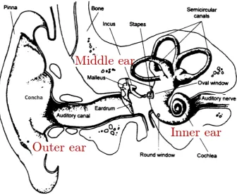
Figure 2.1: Structure of the outer, middle and inner ear. Adapted from Moore (2013).

(18)

nerve. Details of these three components are discussed in the following sections.

2.2.1

The outer ear

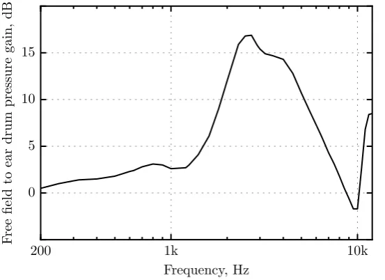
The pinna (auricle) and auditory canal (meatus) make up the outer ear. The pinna is the visible part of the ear outside of the head and is made up of different structural components. In addition to protecting the middle and inner ear, the pinna collects sound waves over a large area and directs them to the eardrum. This, along with the resonances created by the cavities of the external ear, creates a frequency-dependent gain in pressure at the eardrum, increasing the energy transfer to the middle ear. The ear canal, approximately 2.3 cm in length in humans, is often modelled as a quarter-wavelength resonator with one open end and one closed end. The concha extends the effective length of the tube, leading to a major resonance at 2.5 kHz with a peak gain between 15 and 20 dB. A second peak at 5.5 kHz is present due to the resonance of the concha. The complex structure of the external ear yields a relatively steady increase in pressure over 2– 7 kHz. Figure 2.2 shows the average pressure gain of the outer ear as a function of frequency according to Shaw’s summary of acoustic measurements performed in 12 different studies (Shaw 1974; Shaw and Vaillancourt 1985). The peak at 2.5 kHz is independent of the direction of the sound relative to the head. At higher frequencies, however, the transfer function changes with the angle of incidence because of the interaction between incoming sound and the complex structures of the pinna. As described in Section 2.3.4, these direction-dependent spectral contours provide important localisation cues, especially for identifying the elevation of a sound.

200 1k 10k

Frequency, Hz 0

5 10 15

F

ree

field

to

ear

drum

pressure

gain,

dB

Figure 2.2: Transfer function of the outer ear (ratio of sound pressure in the free field to sound pressure at the eardrum) at an azimuth of 0° (directly in front of the head). Data from Shaw (Shaw 1974; Shaw and Vaillancourt 1985).

2.2.2

The middle ear

(19)

resulting from the large surface area of the eardrum relative to that of the oval window. The middle ear comprises three ossicular bones: the malleus, the incus, and the stapes. Collectively, the ossicles form a lever action that increases force and decreases velocity at the stapes which connects to the oval window, causing it to vibrate which in turn causes the fluids of the inner ear to move. This lever action also contributes, though to a lesser extent, to the transmission of acoustic energy to the cochlear fluids.

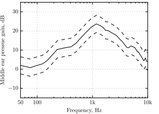
The transmission of sound through the middle ear varies with the frequency of the stimulus. At low to mid frequencies, pressure transfer is determined by the stiffness of the middle ear structures (elasticity in tympanic membrane and ligaments of ear bones) and by the compression and expan-sion of air inside the cavity. Transmisexpan-sion at high frequencies is limited by the mass of the ossicular structure and is also affected by the vibratory patterns of the eardrum breaking up into zones. This frequency dependency can be examined by calculating the transfer function of the middle ear, defined as the ratio of the sound pressure in the scala vestibuli of the cochlea to the sound pressure in the ear canal. For example, Figure 2.3 shows the average transfer function of the middle ear in 11 human ears (Aibara et al. 2001). The average transfer function over 0.05–10 kHz is given by the solid curve and shows a bandpass characteristic with a peak of 23.5 dB at 1.2 kHz. The dashed lines represent an average standard deviation (SD) derived from Aibara et al. (2001). The authors reported approximate slopes of 6 dB/octave from 0.1 to 1.2 kHz and -6 dB/octave above 1.2 kHz. Interestingly, more recent data from the same laboratory showed a shallower high-frequency roll-off of about -2 dB/octave (O’Connor and Puria 2006).

50 100 1k 10k

Frequency, Hz

−10 0 10 20 30

Middle

ear

pressue

gain,

dB

Figure 2.3: Mean (solid) and SD (dashed) transfer function of 11 human middle ears. Data based on Figure 6 (A) of Aibara et al. (2001).

(20)

2.2.3

The inner ear

The inner ear comprises three parts: the semicircular canals, the vestibule and the cochlea. The semicircular canals (superior, posterior and lateral) open into the vestibule, utricle and saccule. These structures are collectively known as the vestibular system which affects the sense of balance. The stapes footplate of the middle ear connects to the oval window of the vestibule—the central cavity of the inner ear. The primary organ of the auditory system is the cochlea, the role of which is to transform vibrations at the stapes into neural information and is the main topic of this section.

Figure 2.4: (a) Path of vibrations in the unrolled cochlear duct. (b) Cross section of the cochlear duct depicting the three scalae and related structures. Adapted from Pickles (2008).

The cochlea is a coiled structure about 1 cm wide and 3 cm when elongated (see Figure 2.4(a)). It is divided by the basilar membrane and Resissner’s membrane into three scalae: the scala vestibuli, the scala tympani and the central scala media or cochlear duct (see Figure 2.4(b)). The two outer scalae (vestibuli and tympani) contain the fluid perilymph, which is near the potential of the surrounding bone, and are joined at the apex by an opening called the helicotrema. In contrast, the inner compartment, the scala media, contains the fluid endolymph which is at a high positive potential (+80 mV) and does not communicate directly with the other scalae. This electrochemical potential difference is responsible for the generation of neural activity in the hair cells and auditory nerve.

The basilar membrane

(21)

Figure 2.5: Schematic of the cochlea showing instantaneous patterns (solid) and envelopes (dashed) of a 60 Hz and 2 kHz travelling wave. Peak displacement is shown by the highest point of the envelope, which is near the apex for low frequencies and near the base for high frequencies. Adapted from Yost (2007).

important points:

1. As the frequency of the tone increases, the position of maximum displacement shifts from the apical end towards the basal end of the cochlea.

2. Because lower-frequency tones travel farther along the membrane, they stimulate both the basal region as well areas near the apex (at peak excitation). In contrast, high-frequency stimulation is concentrated at the base of the cochlea.

Consider the second schematic of Figure 2.5 and imagine a probe measuring the response of the basilar membrane at the location corresponding to the peak excitation (envelope maximum in the schematic). For a pure tone stimulus presented at a constant input level to the cochlea, maximum displacement would occur at a frequency of 2 kHz. Because lower frequencies also gener-ate waves that travel past the same location (see the response at 60 Hz), membrane displacement would also be measured at the same location for tone frequencies lower than 2 kHz, though to a lesser extent. However, frequencies above 2 kHz do not stimulate the measurement point to the same degree because the apical end of the envelope decays much rapidly relative to the basal end. Therefore, the frequency response of the basilar membrane at a particular location shows a bandpass characteristic.

(22)

(a) (b)

Figure 2.6: (a) Velocity of chinchilla basilar-membrane response to tone pips as a function of stimulus frequency and intensity. The measurement was taken at 3.5 mm from the base of the cochlea, which corresponds to a CF of 10 kHz. (b) Velocity of basilar-membrane response to tones with frequency equal to and lower than CF. The straight dashed line has a slope of 1 (dB/dB). Adapted from Ruggero et al. (1997a).

decreases, becoming linear at very low frequencies, as reflected by the straight dotted line. Two primary functional consequences of the nonlinearity near CF is the reduction in input dynamic range inside the cochlea and the production of distortion products. A compressed dynamic range allows perception to operate over a wide range of stimulus intensities but consequently generates audible distortion products which influence perception.

As mentioned, the sharp tuning at CF occurs at low intensities and diminishes at high intensities where the response becomes much broader and takes on a lowpass function. A popular explanation for the mechanism driving this effect is that the healthy cochlea makes use of an active process determined by the outer hair cells. At low stimulus intensities, energy is fed back into the travelling wave, increasing the amplitude of the input vibration. This localised amplification generates a sharply tuned response. As the level of stimulation increases, amplification decreases, causing the response to grow at a rate that is slower than the input. At high levels of stimulation, the cochlear amplifier provides little further contribution and so the input-output behaviour returns to linearity. Because compression mainly occurs near the peak of the vibratory pattern, only frequencies near CF experience this nonlinearity.

In short, each point on the basilar membrane in a healthy cochlea is sharply tuned at low levels, responding to a select range of frequencies. At mid-range levels, the response of the membrane is compressive for stimulus frequencies near CF, effectively broadening the tuning. It should be noted that the pattern of responses are less consistent at the apical end of the basilar membrane. The amount of compression appears to be less than at the base and does not depend as much on the input frequency relative to CF; the frequency-dependency of compression is more broadly tuned.

The organ of Corti

(23)

in the shape of a ‘V’. The tectorial membrane is positioned above the organ of Corti and contacts the stereocilia of the outer hair cells.

The hair cells and supporting cells contain the necessary proteins for establishing high sensitivity of the cochlear structures to biomechanical vibration. Vibration of the stapes causes a travelling wave on the basilar membrane which leads to a bending of the cilia of hair cells. The shearing of stereocilia initiates a neural response in the auditory nerve. It is the difference in pivot points between the tectorial membrane and the basilar membrane that cause this shearing. The cilia of the outer hair cells are bent as a consequence of direct contact with the tectorial membrane. In contrast, it is the fluids trapped between the stereocilia and tectorial membrane that affects the inner hair cells. The shearing of stereocilia is transduced into neural activity by a change in permeability of the hair cell. Tip links are strength-enhancing cross bridges that connect to stereocilia and help to open and close ion channels at the top of the hair cell. This allows for the transport of sodium and potassium ions, thus initiating the neural transduction process.

The majority (85–95%) of afferent nerve fibres are radial fibres which connect to the inner hair cells. These fibres are responsible for carrying sensory information from the organ of Corti to the brainstem and brain. The inner hair cells are therefore the major mechanism for conveying aural information about the incoming stimulus.

When stimulated, the outer hair cells expand and contract. Their change in length influences the vibratory pattern occurring within the cochlear structures. As discussed, this establishes an active mechanism whereby the outer hair cells respond to movement by changing the mechanical coupling between the basilar membrane and tectorial membrane. The sensitivity of the cochlea is amplified as a result of this feedback, thus transducing small vibrations into neural impulses via the inner hair cells. In other words, the outer hair cells serve to amplify the incoming sound with a sharp tuning. They are the active component responsible for the nonlinearities observed in basilar membrane responses, as discussed above.

Neural responses

(24)

Figure 2.7: Tuning curves measured from single neurons in the auditory nerve of anaesthetised cats. Image from Moore (2013).

The frequency selectivity of a single neuron is best described by a tuning curve which plots threshold as a function of frequency. As with measures of basilar membrane selectivity, the fre-quency at which a neuron is most sensitive (lowest threshold level) is also called the characteristic frequency (CF). Figure 2.7 shows typical tuning curves of neurons with different CFs. The tuning curves show a sharply tuned tip where sensitivity is greatest. The fibres show a bandpass character-istic with a steeper high-frequency slopes compared to the low-frequency slopes (on a logarithmic frequency axis). Because each fibre responds to vibration at a single point on the basilar mem-brane, the tuning curves reflect similar frequency selectivity as measured on the basilar membrane. In short, the response of each auditory nerve shows a bandpass characteristic, the width of which increases with centre frequency (in hertz) and the level of the input stimulus.

Rate-level functions

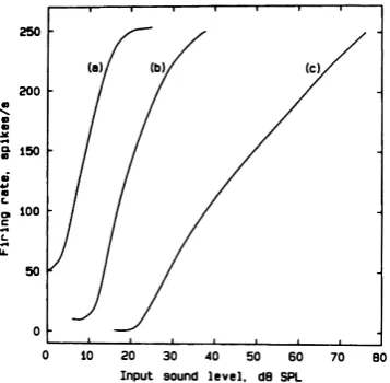
The spike rate of a neuron can be plotted as a function of the input stimulus level to produce a rate-level function. The dynamic range of a neuron is typically about 20 to 50 dB above its thresh-old, after which saturation occurs. However, neuronal dynamic range decreases with increasing spontaneous activity. Thus, neurons with low thresholds tend to have reduced dynamic range compared to those with higher thresholds. Figure 2.8 shows the discharge rate of single neurons as a function of stimulus level. Curves (a)–(c) show responses from neurons with low to high thresh-olds, respectively. Notice that high-threshold fibres show a shallower rate-level function and thus a wider dynamic range at CF. The shallower slopes of these fibres reflect the strong compressive nonlinearity of the basilar membrane intensity functions to CF tones at higher stimulus levels.

Temporal response

Post-stimulus-time histograms (PSTHs) display the number of action potentials or spikes an au-ditory nerve fibre discharges at each moment in time to a repeated stimulus. The spike count is high at the stimulus onset, but decreases rapidly over the first 10–20 ms of stimulation and then drops more steadily. This adaptation effect is illustrated in Figure 2.9 which shows a PSTH to a pure tone burst repeated many times. After the tone offset, the number of spikes fallsbelow the count produced by spontaneous activity, before recovering to the normal rate.

(25)

Figure 2.8: Discharge rate of single neurons as a function of level. Curves (a), (b) and (c) illustrate the response of neurons with high, medium and low spontaneous discharge rates, respectively. The stimulus corresponds to a sinusoid with frequency equal to the CF of each neuron. Image from Moore (2013).

Figure 2.9: Single auditory nerve fibres show an initial sharp onset response to a tone burst, followed by a decrease and finally a transient suppression of spontaneous activity at the offset of the stimulus. This PSTH was formed by repeatedly presenting a tone burst and counting the number of action potentials at each point in time. Image from Pickles (2008).

(26)

Figure 2.10: Period histogram of an auditory nerve fibre given a low-frequency pure tone. The sinusoids of best fit show that the neural pattern is synchronised with the stimulating waveform, even at high levels where the firing is saturated. Image from Pickles (2008).

distributed throughout the waveform period, no synchronisation takes place because the neuron is unable to follow the temporal trajectory of the stimulus.

Two-tone suppression

Discussion thus far has concentrated on neural activity in response to sinusoids presented at differ-ent frequencies and intensities. Presdiffer-enting a single pure tone with a frequency near a neuron’s CF will cause it to fire above its spontaneous activity rate. In absence of any other sounds, a fibre’s response is always excitatory. However, if two tones are presented simultaneously, then, depending on frequency and level, the spike rate generated by the neuron in response to the first tone may actually decrease. The second tone therefore inhibits orsuppresses the activity invoked by the first tone. This phenomenon is called two-tone suppression and is illustrated in Figure 2.11(a). The area bounded by white circles shows the excitatory tuning curve of a single neuron and the open triangle denotes the level of the probe tone which is typically 10 dB above threshold at the fibre’s

(27)

CF. The rate of discharge increases when a second tone with frequency and level falling within the excitatory area is presented. However, when frequency and level of the second tone are varied to within the suppression regions (shaded areas), the average firing rate recorded with the probe drops by at least 20%.

Two-tone suppression occurs at the mechanical stage and is most likely explained by the active behaviour of the outer hair cells. As the travelling waves generated by two sinusoids overlap, the active amplification near the CF corresponding to the excitatory tone is effectively reduced. The travelling wave produced by the suppressor is filtered out by cochlear mechanics, leaving only the wave due to the suppressed tone, but now at a reduced amplitude. This is illustrated in Figure 2.11(b). Note that this explanation of suppression is only appropriate when the excitatory areas of the suppressor and suppressed tones overlap in the upper suppression area. Low-frequency two-tone suppression is currently not well understood.

2.2.4

Modelling the auditory periphery

Computer models of the auditory periphery have been developed to simulate the response of the ear to arbitrary acoustic signals and gain a better understanding of the mechanisms driving the hearing process. A typical auditory model comprises three key stages. First, the transfer function of the outer and middle ear is modelled, typically using linear time-invariant filters. Some models accommodate different sound fields and allow the direction of the incoming source to be specified, e.g. free field with frontal incidence. Second, the frequency selectivity of the basilar membrane is modelled using a bank of bandpass filters with filter bandwidths that increase with centre frequency in accordance with shapes of isovelocity tuning curves at different points along the basilar membrane. The filters are spaced with a near-logarithmic mapping of stimulus frequency to place of peak excitation on the basilar membrane, called the tonotopic map (see Section 2.3.2). A common filter used to mimic both the bandpass filtering action of the basilar membrane and psychophysical measures of frequency selectivity is the Gammatone filter (Boer and Kuyper 1968; Johannesma 1972; Boer and Jongh 1978; Schofield 1985). The Gammatone was developed to simulate the impulse response of auditory nerve fibres and is advantageous in that it has a simple and efficient time-domain implementation (Slaney 1993). More sophisticated models of the hearing system employ nonlinear and asymmetric filters such as the Gammachirp filter (Irino and Patterson 1997; Irino and Patterson 2001) and the dual-resonance nonlinear filter (Lopez-Poveda and Meddis 2001; Meddis et al. 2001), to more accurately simulate the vibratory patterns on the basilar membrane. In particular, they simulate the change in CF and bandwidth at different stimulus levels at a given cochlear site. In contrast, the Gammatone filter is linear in level and has a symmetric frequency response. The final stage of the auditory periphery model mimics the transduction of mechanical vibration to neural signals at the output of each auditory channel. A simplified model involves half-wave rectification followed by lowpass filtering applied to the output of each channel of the filter bank. As with models of basilar membrane filtering, more complex computational devices have been developed to better represent the stochastic nature of the mechanical to neural transduction that takes place between the inner hair cells and individual auditory-nerve fibres, such as Meddis’ hair cell model (Meddis 1986, 1988).

2.3

Hearing psychology

(28)

to an external stimulus are measured. This procedure can be viewed as measuring an unknown system (the human listener) with inputs and outputs. By carefully manipulating the properties of the input acoustic signal, systematic changes in the response of the listener can be captured and correlations can be made. By conducting different experiments and relating findings with physiological measurements, one can develop an understanding of the mechanisms driving per-ception and establish models for predicting subjective responses to new sounds. The aim of this section is to provide the reader with an overview of key findings from experiments concerned with cognitive responses to sound. In particular, the fundamentals of psychoacoustics are summarised: perceptual thresholds, critical bands and masking, loudness perception, and spatial hearing. An understanding of these topics is imperative for developing models and applications founded on auditory perception.

2.3.1

Absolute thresholds

The absolute threshold of a sound is the minimum detectable SPL of the sound in the absence of any other sounds. There are two common methods for measuring absolute threshold. The first uses a probe microphone placed close to the listener’s eardrum with the stimulus typically presented through headphones. When measured this way, the threshold is called the minimal audible pressure (MAP). The second approach is to measure the threshold of the sound presented via loudspeaker in a controlled sound field, such as an anechoic chamber. In the absence of the listener, the sound pressure measurement is made at the point corresponding to the centre of the listener’s head when present. This form of threshold is called the minimal audible field (MAF). Thresholds of pure tones at different frequencies produce audibility curves (either MAP or MAF) that characterise the frequency-sensitivity of the human ear in a given listening condition.

20 100 1000 10000

Frequency, Hz

−20 0 20 40 60 80 100

Lev

el

at

threshold,

dB

SPL

Figure 2.12: Threshold of hearing for pure tones presented binaurally in the free field with frontal incidence. The black solid curve shows the threshold data of ISO 389-7 (2005). The red dotted curve is the approximation given by Equation 2.16.

(29)

(RMSE) = 2.1 dB) according to the formula

AT hQ(f) =−5.92 log10(f)3+ 66.34 log10(f)2−243.84 log10(f) + 296.12 +e(6900f )

1.5

−10e−5(3600f −1) 2

,

(2.16)

wheref is frequency in Hz. The approximation is a modification of the function proposed by Ter-hardt (1979) to better account for the more recent data published by the International Organization for Standardization (ISO) in 2005.

The MAF curve illustrates that the human ear is not equally sensitive to pure tones at different frequencies; if it were, the threshold would be a constant level irrespective of frequency. Hearing sensitivity drops off at low and high frequencies and so the audibility curve shows a smooth bandstop characteristic. For example, as the tone frequency decreases below about 1 kHz, the stimulus must be presented at an increasingly higher intensity in order to be detected by the listener. The acoustic effects of the head, torso and middle ear are partly responsible for this nonuniform frequency sensitivity. Recall that the outer ear enhances sound level in the 2–7 kHz region, peaking at around 2.5 kHz (Figure 2.2). In combination with the optimum efficiency of the middle ear at mid frequencies (Figure 2.3), this explains why the audibility curve shows a global minimum near 3 kHz where hearing sensitivity is highest. The marked increase in threshold at very low and high frequencies is partly accounted for by the reduced efficiency of the middle ear. However, the active cochlear amplifier is less effective at frequencies below 500 Hz, which explains why the audibility curve is steeper than the transfer function of the middle ear at low frequencies (Moore et al. 1997).

The MAF (sound-field) and MAP (headphones) contours differ in shape because the former are dependent on the physical characteristics of the listener. In particular, the MAP is somewhat smoother than the MAF at frequencies above 1 kHz, whereas the MAF shows a marked dip at 3– 4 kHz. Furthermore, MAP thresholds represent monaural-listening conditions and MAF represent binaural-listening conditions. Compared to the average monaural threshold, the average MAF threshold is about 2 dB lower as a result of both ears being used. It is also worth noting that there is large inter-subject variability in measurements of absolute threshold—some individuals differ by as much as_±20 dB from the reference contour shown in Figure 2.12. Note also that because of this strong between-subject variation, sound levels are often made relative to the audibility threshold of a specific individual and are expressed as a sensation level in dB. Thus, two sensation levels of 10 dB measured from two different subjects indicates that the stimulus was presented 10 dB above their respective absolute threshold, which may not be equivalent in SPL. This representation effectively normalises the data for inter-subject differences in detectability.

2.3.2

Masking

(30)

be increased to achieve detectability; thus, the threshold of audibility has been raised. If this new threshold—the masked threshold—is now, for example, 10 dB SPL, then the amount of masking is the difference between the masked and unmasked (in quiet) threshold. In this example, the amount of masking is 7.6 dB.

There are two types of auditory masking: simultaneous masking and nonsimultaneous (or temporal) masking. The first refers to the case where both signal and masker are presented at the same time, and it is primarily the spectral relationship between the two that determines the amount of masking. The second type of masking happens when the signal and masker do not co-exist in time; the masker can still affect the perception of the signal if the masking stimulus is presented before the onset or after the offset of the signal. In this section, the concept of the critical band is introduced, followed by a summary of perceptual phenomena relating to the two types of masking.

Critical bands

The frequency resolution of the hearing system is primarily determined by the tuning of the neural transduction process. As discussed in Section 2.2.3, different frequencies excite different positions on the basilar membrane, with low frequencies stimulating the apical end of the cochlea, and high frequencies stimulating the basal end. Because the hair cells lie along the length of the membrane, this frequency-to-place conversion establishes a neural encoding of sound that is tonotopically organised. Furthermore, the response of the basilar membrane at a given site is frequency selective or tuned, and therefore the sensitivity of a single auditory nerve fibre is also dependent on the frequency of the stimulating waveform. As discussed, neural tuning curves show a bandpass characteristic with maximum sensitivity at a specific frequency. The hearing system is therefore said to behave as though it contains a set of spatially organised bandpass filters known as the auditory filters or critical-band filters. This filtering is responsible for the frequency-resolving power of the ear.

Fletcher (1940) assumed that the auditory filter was rectangular and conducted experiments in which the threshold of a pure tone was measured in the presence of a narrowband masking noise. Threshold was measured as a function of the noise bandwidth, keeping the spectral density constant, i.e. the overall level of the noise increased with bandwidth. Fletcher found that signal threshold increases with the bandwidth of the noise, but flattens off as the bandwidth exceeds a critical point, known as the critical bandwidth. In other words, increasing the noise bandwidth beyond a specific point no longer affects the detectability of the tone, despite the overall intensity of noise continuing to grow. An example threshold measurement according to this procedure is shown in Figure 2.13. Although Fletcher’s band-widening experiment leads to systematic errors in the estimation of the bandwidth of the auditory filter, it is nonetheless important because it has led to the widely accepted power-spectrum model of masking (Patterson and Moore 1986). In essence, this model assumes that the auditory system is made up of a series of overlapping bandpass filters and that, when detecting a signal in noise, the listener makes use of a single filter centred close to the signal frequency. Furthermore, it is assumed that only components falling within the auditory filter centred on the signal frequency contribute to masking. Signal threshold is determined by the signal-to-noise ratio at the output of the filter, based entirely on long-term-power spectra (component phases and short-term fluctuations are discounted).

(31)

50 100 200 400 800 1600 3200

Bandwidth of masking noise, Hz 70

71 72 73 74 75 76

Signal

threshold,

dB

SPL

Figure 2.13: Threshold of a 2 kHz pure tone plotted as a function of the bandwidth of a noise masker centred at 2 kHz. Image redrawn from Moore (1995).

white noise masker is denotedN0, then the total power in the filter is given by

PN =N0

Z ∞

0 |

H(f)_|2df. (2.17)

Given that the filter is rectangular, the power can be expressed as

PN =N0B, (2.18)

whereB is the filter bandwidth. Fletcher assumed that, at masked threshold, the signal-to-noise ratiok was constant,

k= PS

PN

, (2.19)

and therefore that

B= PS

kN0

. (2.20)

By assuming that k= 1, Fletcher could measure the critical bandwidth using PS/N0, known as the critical ratio. Unfortunately, the critical ratio is known to vary with measurement method and more recent experiments have shown the value ofk to be around 0.4 and also to vary with frequency (Moore 1995).

In reality, the critical bands are not rectangular but this representation is convenient when expressing the bandwidths of real filters. The critical bandwidth is a measure of the effective bandwidth of the auditory filter if it were rectangular in shape with a maximum value of one. The equivalent rectangular filter should therefore pass the same amount of power as the real filter. It is for this reason that the bandwidth is also called the equivalent rectangular bandwidth (ERB) of the auditory filter.

Psychophysical tuning curves

(32)

sensitivity of a single neuron to different stimulating frequencies; a neuron is most sensitive to a particular frequency, and as the frequency of stimulus changes, higher levels of stimulation are required to reach threshold. Similarly, the selectivity of the ear at a given place can be measured psychophysically through simultaneous masking. A psychophysical tuning curve (PTC) is typically measured by using a low-intensity pure tone as the target stimulus and either a short-duration sinusoid or narrowband noise as the masking stimulus. The masked threshold is then measured as a function of level and frequency of the masker. It is assumed that the masker produces a constant output from the auditory filter centred at the frequency of the target stimulus. The PTC therefore defines the level of the masker required to produce a constant output from the auditory filter as a function of frequency. Example PTCs are shown in Figure 2.14.

Figure 2.14: PTCs derived from a simultaneous masking experiment involving 50 ms pure tones fixed at a sensation level of 10 dB. The solid circle below each curve indicates the SPL and frequency of the target tone. The masker was a sinusoid and the masked threshold was measured with the masker set at different frequencies. The dashed line corresponds to the absolute threshold for the target tone. Image from Moore (2013).

(33)

Figure 2.15: Illustration of the notched-noise method for measuring the shape of the auditory filter. Image from Moore (2013).

The notched-noise method

Patterson (1976) established a technique called the ‘notched-noise method’ to measure the shape of the auditory filter, whilst controlling for off-frequency listening. In this paradigm, illustrated in Figure 2.15, a notched-noise masker is centred on the frequency of the pure tone. Signal power at detection threshold is then recorded as a function of the notch width 2∆f. Because noise is placed either side of the tone frequency, the listener is forced to use an auditory filter located in the notch, presumably close to the frequency of the signal. As the width of the notch increases, less noise passes through the filter and so threshold level decreases (less masking). Compared to Fletcher’s method, the notched-noise experiment has the advantage of measuring the shape of the filter and providing an estimate of the signal-to-noise ratiokat threshold.

At moderate noise levels, the shape of the auditory filter is near enough symmetric on a linear frequency scale. The power of the signal at thresholdPS can then be obtained by integrating the

power of the notched noise, centred at frequencyfc with a width of 2∆f, passing through both

sides of the filter

PS=kN0

Z fc−∆f

0

df_|H(f)_|2₊_kN 0

Z ∞

fc+∆f

df_|H(f)_|2_. _(2.21)

The integral represents the total area of the noise passing through the filter, depicted by the shaded areas in Figure 2.15. Because this function measures the integral of the filter at a given frequency deviation ∆f, the shape of the filter_|H(f)_|2_{can be derived directly from the slope of the threshold} curve. Patterson and Nimmo-Smith (1980) argued that the rounded exponential (roex) function provided the most successful representation of the filter shape. The simplest of the family of roex functions is

|H(f)|2_{= (1 +}_pg₎_e−pg_, _(2.22)

wheregis the normalised deviation of the frequency from the centre frequency of the filter

g= |f−fc|

fc , (2.23)

andpdefines the critical bandwidth. The filter is called the roex(p) filter because it has only one parameter (p). The larger the value ofp, the more sharply tuned the filter. The area under the function is 4/pand so the ERB is 4fc/p.

(34)

lower sidepland one for the upper sidepu. The ERB of the roex(pl, pu) filter is then (2/pl+2/pu)fc.

Results show that the upper skirt of the filter becomes slightly steeper with increasing level, though this effect varies with frequency, and that the lower skirt becomes shallower (Moore and Glasberg 1987; Glasberg and Moore 1990).

Critical bandwidth

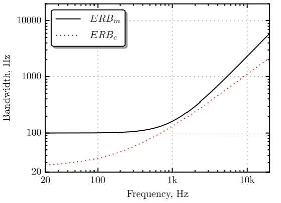
Since the 1950s, many experiments have been conducted to measure the critical bandwidth or ERB of the auditory filters. The critical bandwidth describes the width of the critical-band filter at a given frequency. The most popular critical bandwidths are those defined by the Bark scale published by Zwicker (1961). The ERB according to Zwicker is

ERBm(f) = 25 + 75 1 + 1.4

_f

1000

2!0.69

, (2.24)

wheref is the frequency of the critical band in Hz. Following a similar convention as Hartmann (1998), the subscriptmis used to emphasise that this is a measure of bandwidth for the ‘Munich’ critical bands as measured in Germany.

The Bark scale (in units of Bark) defines the number of critical bands below a given frequency and as such is a transformation of linear frequency,

zm(f) = 13 arctan(0.00076f) + 3.5 arctan (f /7500)2. (2.25)

It is assumed that a constant increment in Bark corresponds to a constant distance along the basilar membrane. Equation 2.25 therefore establishes a relationship between stimulus frequency and place of peak excitation on the basilar membrane. The width of each critical band corresponds to a fixed distance along the basilar membrane of 1.3 mm. There are a total of 24 abutting critical bands according to the Bark scale.

Moore and Glasberg (1983) summarised results from masking experiments where the shape of the auditory filter was measured using the notched-noise and the rippled-noise method. Their find-ings indicated that unlike Zwicker’s expression of the critical bandwidth, the width of the auditory filter continues to decrease at centre frequencies below 500 Hz. For normal-hearing listeners, their revised ERB function is (ANSI S3.4 2007)

ERBc(f) = 24.673(0.004368f+ 1), (2.26)

where the subscript c is used to differentiate from Equation 2.24, since the measurements of the auditory filter shapes were carried out in Cambridge, UK.

The two ERB formulae are compared in Figure 2.16. At frequencies above 500 Hz, the band-widths defined by Zwicker (Equation 2.24) and Moore and Glasberg (Equation 2.26) are similar except that the latter are narrower. At lower frequencies, the function according to the Bark scale tapers towards a fixed value of 100 Hz, whereas ERBc continues to decrease. Moore and Glasberg

(1997) state that at low frequencies, the methods from which Zwicker’s critical bandwidth function was derived are affected by factors other than frequency sensitivity and that later studies employ-ing more controlled methods show a continuemploy-ing decrease in bandwidth for centre frequencies below 500 Hz.

(35)

20 100 1k 10k

Frequency, Hz 20

100 1000 10000

Bandwidth,

Hz

ERBm

ERBc

Figure 2.16: ERB as a function of centre frequency according to Zwicker (ERBm), and Moore and

Glasberg (ERBc).

below a given centre frequency,

zc(f) = 21.366 log10(0.004368f+ 1). (2.27) As a result of the narrower bandwidths defined by Equation 2.26, more (non-overlapping) filters are required to cover the audible frequency range - approximately 41 on the Cam scale compared to 24 on the Bark scale.

Masking patterns

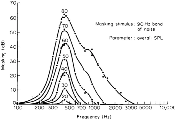
Simultaneous masking is also referred to as frequency or spectral masking, because the amount of masking is dependent on the spectral relationship between the masker and signal. For example, a narrowband noise centred at the same frequency of a pure tone is much more effective at masking the tone compared to a noise centred an octave higher. Figure 2.17 illustrates this by showing

masking patterns derived from an experiment whereby a narrowband noise centred at 410 Hz

served as the masking stimulus and the threshold of a pure tone was measured as a function its frequency. In this case, as was done in many early experiments investigating frequency masking, it is the signal frequency that is varied while the masker is held constant.

Masking is most effective when the frequency of the tone is close to the centre frequency of the masking noise. Additionally, the masking pattern becomes progressively asymmetrical as the level of the masker increases: the upper slope of the masking pattern becomes shallower. This means that an increment in the level of the masker raises the masked threshold by a greater amount at higher frequencies. Consequently, high-frequency signals are more susceptible to masking caused by lower frequency maskers than vice versa, especially at high-intensity levels. This nonlinear growth in masking is referre