Pipe failure prediction in water distribution systems considering static and dynamic factors

(1)

Procedia Engineering 186 ( 2017 ) 117 – 126

Peer-review under responsibility of the organizing committee of the XVIII International Conference on Water Distribution Systems

doi: 10.1016/j.proeng.2017.03.217

ScienceDirect

XVIII International Conference on Water Distribution Systems Analysis, WDSA2016

Pipe Failure Prediction in Water Distribution Systems Considering

Static and Dynamic Factors

Raziyeh Farmani

a

_{*, Konstantinos Kakoudakis}

b

_{, Kourosh Behzadian}

c

_{and David Butler}

d

a_{Associate Professor, Centre for Water Systems, University of Exeter, Exeter, UK} b_{PhD student, Centre for Water Systems, University of Exeter, Exeter, UK}

c_{Senior Lecturer, University of West London, London, UK} d_{Professor, Centre for Water Systems, University of Exeter, Exeter, UK}

Abstract

Due to high economic, environmental and social costs resulting from pipe bursts in water distribution systems, development of a reliable and accurate prediction model to assess susceptibility of a pipe to failure is of paramount importance. This paper aims to consider the impact of both static and dynamic factors on pipe failure for long and mid-term predications. Length, diameter and age of pipes are the static and weather is the dynamic factors for the prediction model. To improve the performance of the pipe failure prediction models, the K-means clustering approach is considered. Evolutionary Polynomial Regression (EPR) is used as the pipe failure prediction model. To prepare the database for the prediction model, homogenous groups of pipes are created by

aggregating individual pipes using their attributes of age, diameter and soil type. The created groups were divided into training and test datasets using the cross-validation technique. The K-means clustering approach is employed to partition the training data into a number of clusters with similar features based on diameter and age of the pipe groups. An EPR model is developed and calibrated for each data cluster. To predict pipe failures for new (unseen) data, the most suitable cluster is identified and the relevant EPR model is used to obtain the most accurate prediction. The proposed approach is demonstrated by application to a water distribution system in the UK. Comparison of the results shows that the cluster-based prediction model is able to significantly reduce the prediction error of pipe failures. Temperature-related factor is identified as the main dynamic factor influencing the t mid-term prediction of pipe failures. An EPR model is employed to predict the annual variation in the number of failures. Mid-term and long-Mid-term prediction models are developed to present the relationship between number of pipe failures and temperature-related factors for better operation and long term for capital investment respectively.

* Corresponding author. Tel.: +44 1392 723630 E-mail address: [email protected]

(2)

Keywords: water distribution system; pipe failure; prediction models; Evolutionary polynomial regression; K-means clustering

1. Introduction

The failure of water distribution networks’ pipes is a global concern due to the potential consequences. The water

authorities, in order to cope with pipe failure, can follow either a reactive or a proactive approach. In a proactive strategy pipe rehabilitation is scheduled in advance after assessing and forecasting pipe propensity to fail [1]. The proactive strategy includes scheduling the maintenance, improvement and extension of water mains in order to maintain/improve the current level of service. The use of predictive models is an important step in the implementation of the proactive strategy. They can help water utilities to make more informed and accurate decisions for the future planning of pipe rehabilitation and/or replacement.

The pipe failure is the cumulative effect of various pipe-intrinsic (such as material, diameter, and age), operational (such as corrosion, pressure, external stresses) and environmental factors (such as temperature, rainfall, soil conditions) acting on them. Environmental and pipe-intrinsic factors can be divided into static and dynamic (time-dependent), while operational factors are inherently dynamic. This paper proposes the use of two different approaches for the long-term and the mid-term prediction of pipe failure. The prediction models provide insights into the relationships between pipe failure and all kinds of factors influencing pipe failure. The long-term approach employs the pipe-intrinsic factors as explanatory variables while the mid-term approach employs the environmental factors.

The paper presents the combined use of Evolutionary Polynomial Regression [2] and K-means clustering method [3] to achieve accurate long-term predictions of the expected number of pipe failures. The mid-term approach uses EPR to predict the number of failures yearly considering weather-related factors as explanatory variables.

2. Methodology

Figures 1&2 show the framework for the long-term and mid-term prediction of pipe failures. The long-term prediction models consider length, diameter and age and the mid-term prediction models g temperature-related factors as explanatory variables respectively. The prediction models were developed using EPR-MOGA-XL vr.1 [4, 5].

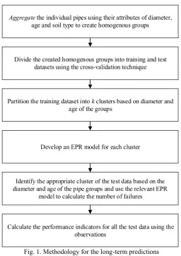
The proposed methodology for the long-term predictions consists of the following steps (figure 1):

Initially, the individual pipes are aggregated into homogenous groups assuming that pipes with similar specific intrinsic properties such as material, diameter and age are expected to have the same breakage pattern [6]. In addition, soil type is used as an aggregation criterion because soil properties have been associated with the corrosion of the metallic pipes [7, 8] and are considered as a major factor contributing to their failure [9, 10]. The total length and the total number of failures of each homogenous group (specific age, diameter and soil type) are calculated as a sum. The original database which includes a huge number of individual pipes is converted into a number of groups.

The created homogenous groups were split into training and test datasets using the cross-validation technique [11] for calibration and validation purposes respectively. All the groups are used both for training and test and each group is used for test exactly once [12]. The training dataset is partitioned into k clusters based on diameter and age of groups using the K-means algorithm. One EPR model is developed for each cluster of the training dataset.

Finally, the performance of the developed models is evaluated by using the test data. The Euclidian distance between the test data sample (i.e. age and diameter of the groups that constitute the test dataset) and the counterpart cluster centre values is calculated to identify the appropriate cluster for each test data. The corresponding model is employed to calculate the number of failures and the performance indicators are evaluated using the predicted values and the observations.

(3)

Fig. 1. Methodology for the long-term predictions

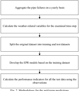
The proposed methodology for the mid-term predictions consists of the following steps (figure 2):

The first step is the aggregation of pipe failure and the definition of the climate-related variables. Daily climate data for the area examined were obtained from the British Atmospheric Data Centre (BADC) (http://badc.nerc.ac.uk/home/index.html) and consisted of minimum, average and maximum air temperatures (0_{C). To avoid}

negative values, all temperatures were converted to Fahrenheit.

A number of temperature-related factors were examined for their ability to capture the variation in the annual number of failures. The covariates considered are: average minimum air temperature (eq. 1), average maximum air temperature (eq. 2), average mean air temperature (eq. 3) and freezing index (eq. 4). The freezing index is defined as the cumulative minimum daily temperature below a specified air temperature threshold and is a surrogate for the duration and severity of extreme air temperatures within a time step. Initially the cross-correlation function in MATLAB (® R2014b) was applied to measure the similarity between the candidate thresholds and the number of failures. The thresholds examined range between -20_{C and 4}0_{C with a step of 1}0_{C. The threshold that provided the}

highest similarity was selected for data aggregation.

ܶ௠௜௡௜௠௨௠=

σ೘_ೕసభ்_{೘೔೙೔೘ೠ೘}ೕ

௠ (1)

ܶ௠௔௫௜௠௨௠=

σ೘_ೕసభ்_{೘ೌೣ೔೘ೠ೘}ೕ

௠ (2)

Develop anEPR model for each cluster

Aggregate the individual pipes using their attributes of diameter, age and soil type to create homogenous groups

Divide the created homogenous groups into training and test datasets using the cross-validation technique

Partition the training dataset into k clusters based on diameter and age of the groups

Identify the appropriate cluster of the test data based on the diameter and age of the pipe groups and use the relevant EPR

model to calculate the number of failures

(4)

ܶ௔௩௘௥௔௚௘=

σ ்ೌೡ೐ೝೌ೒೐ ೕ ೘ ೕసభ

௠ (3)

FI=σ௠ ሺߠ െ ܯ݅݊ܶ௝_ሻ

௝ୀଵ (4)

where m is the number of days in the time step i, ܶ_{௠௜௡௜௠௨௠}௝ is the minimum daily temperature of day j, ܶ_{௠௔௫௜௠௨௠}௝

is the maximum daily temperature of day j and ܶ_{௔௩௘௥௔௚௘}௝ is the average daily temperature of day j andθis the air temperature threshold

The created data (aggregated failure data and candidate explanatory variables) are divided into two parts, 70% and 30% for training and test purposes respectively.

Fig. 2. Methodology for the mid-term predictions

3. Evolutionary Polynomial Regression

Evolutionary Polynomial Regression [2] is a data-driven method based on numerical and symbolic regression able to produce series of pseudo-polynomial models. The user selects the generalised model structure and the EPR employs a multi-objective search strategy to estimate unknown constant parameters of the assumed models using the least squares method. Each single EPR run returns a number of polynomial models on a Pareto optimal front which is a trade-off between accuracy (fitness) and parsimony. The accuracy criterion aims to maximise the model fit to the observed data while the parsimony criterion aims to minimise the number of explanatory variables and/or polynomial terms in the model. In this study, the model is selected considering the number of polynomial terms as a surrogate for the model parsimony criterion. Its role is to prevent over-fitting of the model to data and thus endeavour to capture

Develop the EPR models based on the training dataset Aggregate the pipe failures on a yearly basis

Calculate the weather-related variables for the examined time-step

Split the original dataset into training and test datasets

(5)

underlying general phenomena without replicating noise in data [13]. The general form of polynomial EPR model [2] is expressed as:

Y =σ௠_௝ୀଵܨ൫ܺǡ ݂ሺܺሻǡ ܽ_௝൯ ൅ܽ_௢ (5)

where Y= estimated output; ܽ௝= unknown polynomial coefficients (i.e. model parameters); F= function finally

constructed by the EPR process; X= the matrix of explanatory variables; f= function selected by the user; and m= the maximum number of polynomial terms and ܽ_଴= unknown constant.

The specific model structure selected here for analysis of pipe failure is [2]:

Y =σ௠_௝ୀଵܽ_௝ሺሺܺ_ଵሻாభೕǥሺܺ_௜ሻா೔ೕ_{ሻ ൅ ܽ}

଴ (6)

where Y=predicted number of pipe failures, Xi =is the explanatory variable i and Eij =matrix of unknown exponents

to be calculated.

The candidate values considered for exponents (Eij) in Equation (6) were -2, -1, -0.5, 0, 0.5, 1 and 2 describing potential square, linear or square root exponents for explanatory variables of the EPR model. The value 0 was chosen to deselect input candidates with no influence on the output, while the positive and negative values were considered to describe potential direct and inverse relationship between the inputs and the output of the model. The maximum number of polynomial terms was set to 3 (i.e. m=3) excluding the constant term (ܽ_଴) to ensure the best fit without unnecessary complexity which is defined [14] as the addition of new terms that fit mostly random noise in the raw data rather than the underlying phenomenon. The result of each single EPR run is three regression models corresponding to the maximum number of polynomial terms defined in advance. All the candidate models have different number of polynomial terms (ranging from one to three) and combination of inputs the constant values. The Least Square (LS) method was constrained to search for positive polynomial coefficient values only (i.e. ܽ௝>0)

because negative polynomial coefficients (i.e. ܽ_௝<0) usually try to balance positive terms providing a better description of the noise [15].

4. K-means clustering

The K-means clustering is applied here using the KMEANS function in MATLAB (® R2014b) to partition the training data into a number of specified clusters based on the diameter and the age. Generally, clustering is a data exploration technique that groups objects with similar characteristics together and thus classifies a large number of objects into a small number of clusters in order to facilitate their further processing [16]. The creation of the clusters is based on the principle of maximising the intra cluster similarity and minimising the inter cluster similarity [17]. K -means is an unsupervised learning algorithm popular due to its simplicity and efficiency [18]. It is based on assigning n data samples into k clusterssuch that an objective function of dissimilarity (or distance) is minimised [19]. The search algorithm moves data samples between clusters until the objective function cannot be minimised further. In the case of the dissimilarity measure, minimisation of the Euclidean distance is usually chosen as the objective function as [20]:

J=σ௞_௝ୀଵσ௡_௜ୀଵቚݔ_௜ሺ௝ሻെ ܿ_௝ቚଶ (7)

where ቚݔ_௜ሺ௝ሻെ ܿ_௝ቚଶ= Euclidean distance of specified criteria between ith data sample ݔ_௜ሺ௝ሻ and jth cluster centre

ܿ௝; ݔ௜ ሺ௝ሻ

= vector of specified criteria for ith data sample assigned to jth cluster centre; J=overall distance indicator for the n data samples from their respective cluster centres.

(6)

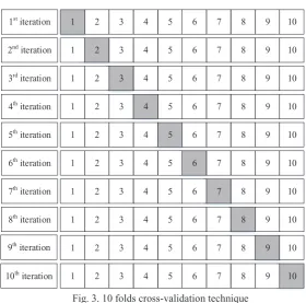
The m-fold cross-validation method [21] used (figure 3) extends the conventional single-split method by dividing the data into m subsets of (approximately) same size. One subset is taken as the test set (shaded area in figure 3) and the remaining m-1 subsets form the training set. This process is repeated with a new subset of the training/test data. The overall performance is calculated by specified performance indicators applied to all data in m individual performance assessments. In this work, m=10 is used as suggested by [21], in which the union of 9 subsets (i.e. 90% of data) is allocated for training and the one remaining subset (i.e. 10% of data) is retained for test. Τhecross-validation method consists of the following steps:

x The grouped dataset of pipe failure is randomly divided into m equal and mutually exclusive folds (here 10) and the training and test subfolders are specified as described above;

x For each sub-fold i, the model is trained using specified training data and evaluated using specified test data; x Step 2 is repeated m times (here 10);

x The overall performance is the average value of the m calculated performance indicators

1 2 3 4 5 6 7 8 9 10

1st_iteration

2nd_iteration

3rd iteration

4th_iteration

5th_iteration

6th_iteration

7th iteration

8th_iteration

9th iteration

10th_iteration

Fig. 3. 10 folds cross-validation technique

The performance indicators used here are the Coefficient of Determination (R2_{) as a measure for correlation} between predictions and observations and Root Mean Square Error (RMSE) as a measure for error prediction. The mathematical relationships of these indicators are expressed as follows [22]:

ܴଶ= ሺσ ሺ௬೛ǡ೔ି௬ത೛ሻሺ௬೚ǡ೔ି௬ത೚ሻ

೙

೔సభ ሻమ

σ೙೔సభሺ௬೛ǡ೔ି௬ത೛ሻమσ೙೔సభሺ௬೚ǡ೔ି௬ത೚ሻమ

(8)

RMSE=ටσ ሺ௬೛ǡ೔ି௬೚ǡ೔ሻ

మ ೙

೔సభ

௡ (9)

(7)

6. Case study

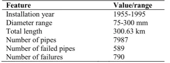
The proposed methodology is demonstrated here for in a case study located in part of a water distribution network (WDN) of a UK city. The database contains a large number of individual pipes made of five different materials. Preliminary analysis showed that the Cast Iron (CI) pipes which constitute 78% of the network’s total length have the

highest pipe failure rate. In addition, pipe records show that 85% of the failed pipes are made of CI pipes. It is concluded that the CI pipes are more prone to failure and therefore only they are considered in this paper for construction of the predictive models. Table 1 shows the main features of CI pipes considered in the case study.

Table 1 The main features of the Cast Iron pipes in the case study

Feature Value/range

Installation year 1955-1995

Diameter range 75-300 mm

Total length 300.63 km

Number of pipes 7987

Number of failed pipes 589 Number of failures 790

7. Results

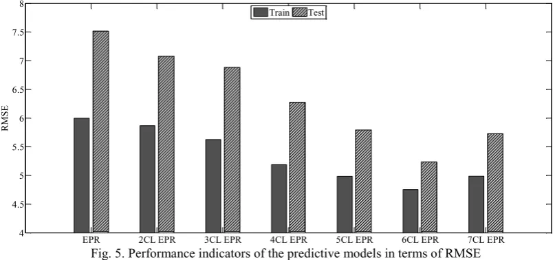
The implementation of long-term approach resulted in three EPR models for each cluster. In order to avoid over-fitting and in compliance with the parsimony rules, one polynomial term EPR model was selected from the Pareto front for all model runs analysed in this paper [23]. The cluster based approach was applied for different numbers of clusters (k) and the most appropriate number of clusters was identified by comparing the performance indicators (figures 4&5). The values shown in figures 4&5 are the average values of the 10 iterations of the cross-validation technique. The results showed that the two performance indicators are improved by increasing the number of clusters until six clusters when no further improvement is achieved for both training and test data with both indicators. The comparison indicates that both performance indicators for the clustered EPR models are better than the non-clustered EPR approach for all the different number of clusters and for both training and test data. More specifically, the comparison of the six-clustered EPR with the non-clustered EPR shows a significant improvement especially for the RMSE (i.e. improvement of 30% with the test data and 20% with the train data). Improvement is also observed for R2

for both train and test data, although lower compared to the RMSE.

Fig. 4. Performance indicators of the prediction models in terms of R2

*CL=abbreviation for ‘clustered’ (e.g. 2CL=two-clustered)

EPR *2CL EPR 3CL EPR 4CL EPR 5CL EPR 6CL EPR 7CL EPR

0.8 0.82 0.84 0.86 0.88 0.9 0.92 0.94 0.96 0.98 1

R

2

(8)

Fig. 5. Performance indicators of the predictive models in terms of RMSE

The improvement obtained can be attributed to the fact that clustered approach would be beneficial for pipe failure analysis and thus more appropriate EPR models fitted to the clustered data are identified effectively.

Table 2 lists the associated models obtained from developing the six-clustered EPR and non-clustered EPR corresponding to one of the ten iterations of cross-validation. In both models, total number of pipe failures (Y) were selected from one polynomial term comprising of total group length (L), the diameter (D) and the age (A) of pipes with the defined candidates of exponents. Note that one polynomial term prediction model was selected and preferred here for all models in order to avoid possible overfitting of test data. The equations obtained (Table 2) show a direct relationship between the pipe failure and the age and an inverse relationship with the diameter for both the approaches.

Table 2. Obtained formulas for six-clustered EPR and EPR models

Six-clustered EPR Non-clustered EPR

Cluster 1: Y=4.324(L0.5_A1.5_D-0.5₎ _Y=0.153(LAD-1₎

Cluster 2: Y=0.956(L1.5_A0.5_D-2₎

Cluster 3: Y=0.476(LA1_D-1.5₎

Cluster 4: Y=1.023(L0.5_A1.5_D-1₎

Cluster 5: Y=0.327(LAD-2₎

Cluster 6: Y=2.851(LA0.5_D-1.5₎

The methodology described in the mid-term subsection was implemented and the EPR models were generated. The model was selected with respect to the goodness to fit the observed data, the parsimony of the equation and the possibility to describe the physical phenomenon. In order to avoid over-fitting and in compliance with the parsimony rules, one polynomial term EPR model was selected [23].

The performance of the selected model (eq. 10) is evaluated using the R2_{and the RMSE. All the performance}

indicators show that the selected model has a high accuracy for both training and test data. More specifically, the ܴଶ

is 0.89 with the train and 0.83 with the test data. The values of RMSE are 7.67 for the train 9.23 and test data respectively.

Y= 5.356ܨܫ଴Ǥହ_+14.695 ₍₁₀₎

The selected model shows that the most important variable is the freezing which is associated with the severity of the cold period. The threshold selected is 00_{C degrees because it provided the highest correlation in the preliminary}

analysis. The selection of freezing index as the most influencial factor can be attributed to the fact the majority of failure occurring the coldest months. The freezing index can more accurately compared to the rest candidate variables capture the variation in the severity of winter.

EPR 2CL EPR 3CL EPR 4CL EPR 5CL EPR 6CL EPR 7CL EPR

4 4.5 5 5.5 6 6.5 7 7.5 8

RMSE

(9)

8. Conclusions

This study presents an approach for the long-term and mid-term prediction of pipe failures. The long-term approach was implemented by combining EPR with K-means algorithm to obtain accurate predictions of failures for homogenous groups of pipes. This was achieved by partitioning the input data into a predefined number of clusters based on pipe characteristics using the K-means algorithm. An individual EPR model was developed for each created cluster and the number of failures were calculated as a function of pipe diameter, age and length from aggregated homogenous pipe groups. The most appropriate cluster for each test data sample was identified based on the closest distance from the cluster centroids and the EPR model associated with this cluster was used for prediction of number of failures. The mid-term approach employed an EPR model to predict the annual number of failures using the weather-related factors as explanatory variables. The following can be concluded from the analyses conducted here:

x The combination of EPR with K-means clustering method results in a considerable improvement of the prediction accuracy for pipe failures when compared to the non-clustered EPR approach.

x The six-clustered EPR approach is capable for prediction of extreme pipe failures (i.e. both small and large number of failures).

x The dynamic weather-related factors can be used to identify the pipe failure trend mid-term.

Acknowledgement

The work reported is supported by the UK Engineering & Physical Sciences Research Council (EPSRC) project Safe &SuRe (EP/K006924/1).

References

[1] J. Røstum, Statistical modelling of pipe failures in water networks, Thesis (PhD). University of Science and Technology, Norway, 2000.

[2] O. Giustolisi, D.A Savic, A symbolic data-driven technique based on evolutionary polynomial regression. Journal of Hydroinformatics, 8 (2006) 207-222.

[3] J. MacQueen, Some methods for classification and analysis of multivariate observations. In Proceedings of the 5th Berkeley symposium on mathematical statistics and probability, 1 (1967) 281-297.

[4] O. Giustolisi, D.A Savic., Advances in data-driven analyses and modelling using EPR-MOGA. Special Issue on Advances in Hydroinformatics, Journal of Hydroinformatics 11 (2009) 225–236.

[5] O. Giustolisi, D.A Savic, D. Laucelli, Asset deterioration analysis using multi-utility data and multi-objective data mining. Journal of Hydroinformatics 11 (2009) 211–224.

[6] Y. Kleiner, B. Rajani, Comparison of four models to rank failure likelihood of individual pipes. Journal of Hydroinformatics, 14 (2012) 659-681.

[7] R. Sadiq, B. Rajani Y. Kleiner, Fuzzy-based method to evaluate soil corrosivity for prediction of water main deterioration. Journal of Infrastructure Systems, 10 (2004) 149–156.

[8] G. Kabir, G. Demissie, R., Sadiq S. Tesfamariam. Integrating failure prediction models for water mains: Bayesian belief network based data fusion. Knowledge-Based Systems. 85 (2015) 159-169.

[9] J.M. Makar, A preliminary analysis of failures in grey cast iron water pipes. Engineering Failure Analysis, 7 (2000) 43-53.

[10] S. Folkman, Water Main Break Rates in the USA and Canada: A Comprehensive Study, Utah State University, Buried Structures Laboratory, Logan, UT, 2012.

[11] R. Grossman, G. Seni, J. Elder, N. Agarwal, H. Liu, Ensemble Methods in Data Mining: Improving 522 Accuracy Through Combining Predictions. Morgan & Claypool, 2010.

[12] T. Gandhi, B.K. Panigrahi, S. Anand, A comparative study of wavelet families for EEG signal classification. Neurocomputing, 74 (2011) 3051-3057.

[13] D. Laucelli, B. Rajani, Y. Kleiner, O. Giustolisi, Study on relationships between climate-related covariates and pipe bursts using evolutionary-based modelling. Journal of Hydroinformatics, 16 (2014) 743-757.

(10)

[15] O. Giustolisi, Α. Doglioni, D.A. Savic, B.W. Webb, A multi-model approach to analysis of environmental phenomena. Environmental Modelling and Software, 22 (2007) 674-682.

[16] D.T. Pham, S.S. Dimov, C.D. Nguyen, Selection of K in K-means clustering. In Proceedings of the Institution of Mechanical Engineers, Part C: Journal of Mechanical Engineering Science, 219 (2005) 103-119.

[17] D. Wettschereck, D.W. Aha, T. Mohri, A review and empirical evaluation of feature weighting methods for a class of lazy learning algorithms. Artificial Intelligence Review, 11 (1997) 273-314.

[18] T. Kanungo, D.M. Mount, N.S. Netanyahu, C.D. Piatko, R. Silverman, A.Y. Wu, An efficient k-means clustering algorithm: Analysis and implementation. Pattern Analysis and Machine Intelligence IEEE, 24 (2002) 881-892. [19] J.S.R. Jang, C.T. Sun, E. Mizutani, Neuro-fuzzy and soft computing; a computational approach to learning and

machine intelligence. Practice Hall, 1997.

[20] S.E. Kim, I.W. Seo, Artificial Neural Network ensemble modeling with conjunctive data clustering for water quality prediction in rivers, Journal of Hydro-Environment Research 9 (2015) 325-339.

[21] R. Kohavi, A study of cross-validation and bootstrap for accuracy estimation and model selection. In Proceedings of the 14th International Joint Conference on Artificial Intelligence, 2 (1995) 1137-1143.

[22] D.N. Moriasi, J.G. Arnold, M.W. Van Liew, R.L. Bingner, R.D. Harmel, T.L. Veith,. Model evaluation guidelines for systematic quantification of accuracy in watershed simulations. Transactions of the Asabe, 50 (2007) 885-900. [23] L. Berardi, Z. Kapelan, O. Giustolisi, D.A. Savic, Development of pipe deterioration models for water distribution